Energy Management Optimization and Voltage Evaluation for Residential and Commercial Areas

Abstract

In most smart grids, load management techniques are required to handle multiple loads of several types. This paper studies decentralized demand-side management (DSM) in a grid with different types of appliances in two service areas: one with many residential households, and one bus with commercial customers. Each building runs an individual optimal DSM to reschedule the usage time of its flexible appliances to reduce its electric energy cost at a manageable sacrifice of inconvenience according to the forecasted time-varying electricity price. Using the developed model, we examined the effectiveness of decentralized DSM by comparing its performance on the operation status of the grid in terms of electricity cost saving, rooftop photovoltaic (PV) utilization efficiency, voltage fluctuation, power loss, voltage rises, and reverse power flows, which can easily be seen at the commercial load bus.

1. Introduction

Demand-side management (DSM) refers to the response taken by the consumer to manage the energy usage based on the electricity price over 24 h [1,2,3,4]. Reference [5] developed an optimization model for a single-household demand-side management (DSM) model. This model, as a single feeder, delivers energy to 13 houses based on a day-ahead household DSM system with local solar photovoltaic (PV) generation. The proposed algorithm searches for the optimal load schedule of the household DSM with solar PV generation, and with multiple technical constraints. Additionally, previous DSM programs used (e.g., References [6,7,8,9,10]) focused on cost minimization. However, demand-side management (DSM) also aims to avoid the peak load during the time of the low electricity price. A combination of time-of-use pricing (TOUP) with a fixed threshold, which represents the maximum load demand applied for each residential household and a commercial site, is illustrated in this paper.

The optimization algorithms used for direct load control schemes are for certain types of loads (for example, refrigerators or air conditioning [11,12,13,14,15]); these algorithms are not suitable for large loads such as commercial or industrial loads. In Reference [16], a strategy of load management was proposed. In this reference, the same electricity price was applied to both residential and commercial areas. For a more realistic study, this paper takes into consideration that residential and commercial loads have different time-varying billing rates and exhibit different characteristics (e.g., power consumption profile, electric devices settings, and customer willingness for DSM participation). Therefore, examining the DSM strategy for both commercial and residential sites is essential in the grid, allowing a comparison of their performance to seek a better management strategy.

The demand-side management (DSM) algorithms used in References [17,18,19,20] are system-specific. These algorithms are not practical for different types of appliances. Reference [9] proposed a DSM model for a residential site. This model aims to minimize the cost based on a day-ahead household DSM system. The proposed algorithm searches for the optimum scheduling of household DSM by doing load shifting to the period with low price, and ensuring the avoidance of any high load occurrences.

Note that the optimization algorithms used for direct load control schemes are for certain appliances (for example, refrigerators or air conditioning [21,22]). Some demand-side management algorithms used in the literature [23,24,25,26,27] are system-specific. These algorithms are not practical for a wide variety of appliances. Our work, however, proposes an algorithm to cover a range of appliances in different types of loads, such as commercial loads and residential loads, despite each type of load having a different characteristic in terms of load profile, electricity price, appliances, and customer willingness for DSM participation.

Unlike the work in Reference [8] that use fixed market prices for both residential and commercial sites, our work uses a time-of-use pricing (TOUP) profile for a residential load that differs from the time-of-use pricing (TOUP) used for a commercial site.

This paper extends the work in Reference [9] to that of a decentralized DSM with multiple residential and commercial loads with a rooftop PV installation. One of the main advantages of the proposed algorithm is the ability to take in to account the voltage fluctuation, in addition to the maximization of PV utilization efficiency, and the reduction of real power loss of the entire system while optimizing the electricity cost. Additionally, the proposed algorithm can handle a large number of controllable appliances in two types of loads: residential and commercial. Furthermore, residential and commercial loads have different time-varying billing rates and exhibit different characteristics, such as load profile, appliance settings, and customer willingness for DSM participation; therefore, they may have different impacts on electricity cost savings and distribution network operation. The designed algorithm handled these complexities successfully, and we examined the DSM performance for both commercial and residential sites to efficiently seek a better management strategy.

This paper proposes a practical model for demand-side management with a flexible penalty approach to account for the inconvenience caused by deviation from the customer-desired schedule. In other words, customer inconveniences caused by the DSM schedule will translate into an additional compensation cost in the optimization objective function, which is calculated based on some customized rate and intends to discourage or reduce unnecessary load shifting or changes.

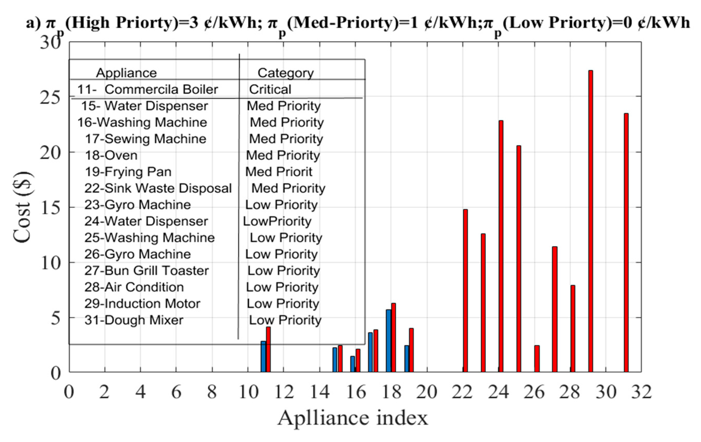
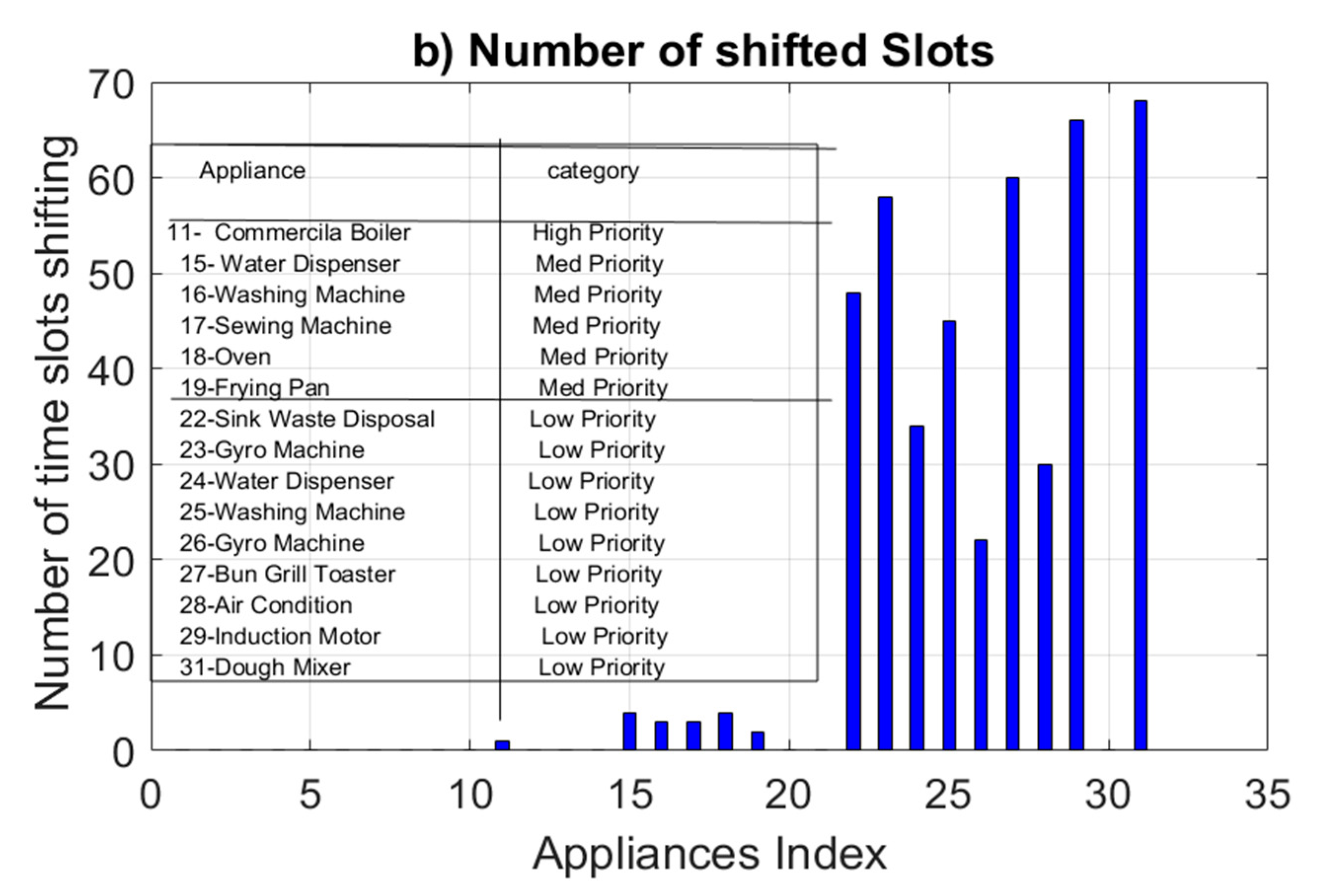
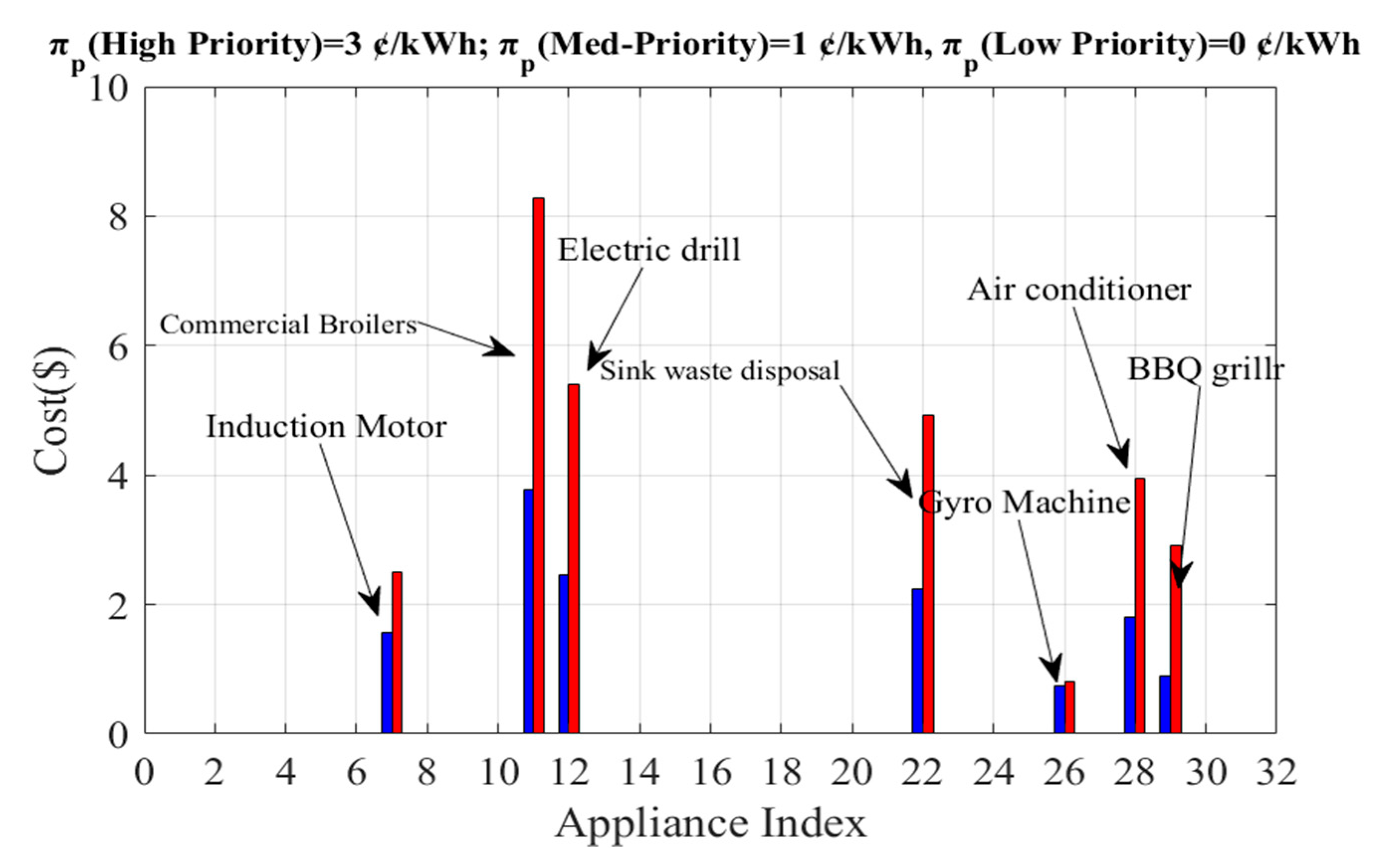
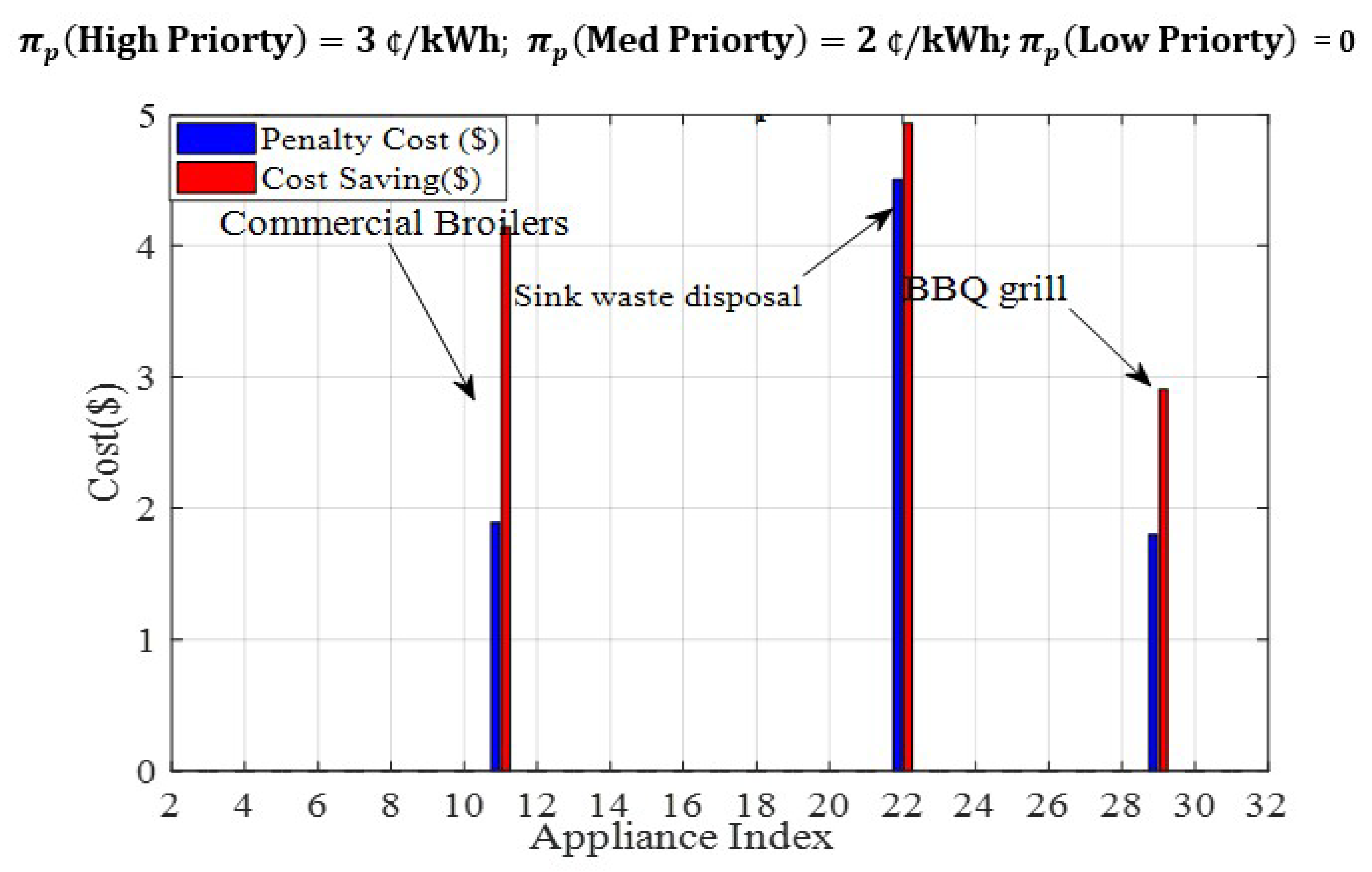
For a more realistic scenario, the proposed algorithm also takes into consideration the fact that certain appliances may have higher priority over other appliances such that these appliances have to operate in their specified time; hence, these types of appliances have less DSM participation. Our algorithm classifies commercial appliances into three categories: high priority, medium priority, and low priority; every kind of appliance is accordingly subjected to a specified penalty price. This also verifies the impact of the penalty price on DSM scheduling of an appliance’s operation.

Our model was verified using the clonal selection algorithm (CSA). This algorithm can deal with multiple types of household appliances in two areas (residential and commercial), despite each type of load having different characteristics such as load profile, electricity price, power rate of the appliances, and customer willingness for DSM participation. The algorithm can evaluate the voltage fluctuation, encouraging solar energy usage, further allowing evaluation of the energy loss while optimizing the electricity cost. The proposed algorithm also takes into consideration the fact that certain appliances may have higher priority over other appliances such that these appliances have to operate in their specified time; hence, these types of appliances are considered as top-priority appliances.

The rest of this paper organized as follows: Section 2 illustrates the model, the decentralized DSM is described in Section 3, the results are summarized in Section 4, and the conclusions are given in Section 5.

2. System Modeling

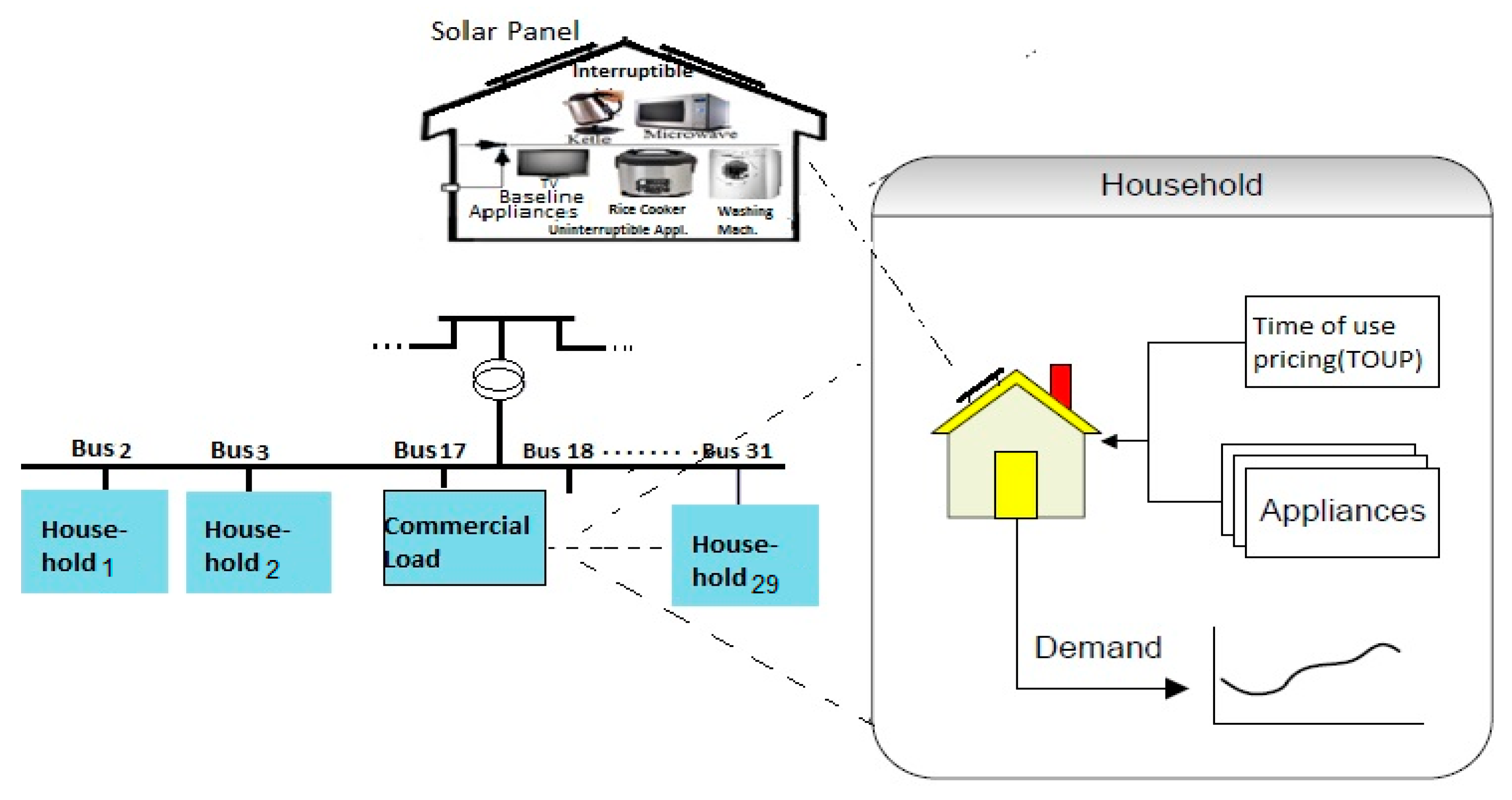
This section clarifies the decentralized DSM in the distribution grid of the feeder to show the influence of the developed DSM model. A DSM is applied on two loads, each with a different type of customer: residential and commercial. As shown in Figure 1, 29 buses represent the households connected in each type. Each household contains different kinds of appliances (see

Table A1. Number (No.) of appliances (appl.) in each residential household. MD—maximum demand.

Bus No.	Interruptible Appl.	Uninterruptible Appl.	MD (kW)
2	21	7	12.4
3	15	4	15.3
4	17	4	11.8
5	12	4	8
6	19	4	10.5
7	21	4	11.5
8	21	4	14.7
9	21	4	15
10	13	4	15
11	18	4	10.5
12	21	7	11.3
13	15	4	13
14	17	4	8.3
15	19	4	13.6
16	21	4	13
18	19	4	11.7
19	18	4	8.6
20	13	4	11.2
21	18	4	9
22	21	7	10
23	15	4	12
24	17	4	7.2
25	19	4	13.6
26	21	4	14
27	21	4	13.8
28	13	4	15.7
29	18	4	8.6
30	21	7	8.3
31	15	4	13

and

Table A3. Parameters of appliances in the residential area.

Categorization of Appliances	Appliance Index	Original Operation Time Slot	${\mathit{D}}_{\mathit{a}} \left(30\right)\min$	Power (kw)	No. of Appliances
Baseline Appliances	1	1−48	48	0.15	150
	2	1−48	48	1.60	150
	3	1−48	48	0.15	150
Uninterruptible Appliances	4	14−17	4	0.73	56
	5	23−25	3	0.73	48
	6	24−26	3	0.80	97
	7	20−22	2	0.80	185
	8	21−22	2	0.8	168
	9	12−15	4	0.38	267
	10	26−29	4	1.26	115
Interruptible Appliances	11	21−24	4	1.26	164
	12	39−42	4	1.64	118
	13	43−46	4	1.26	174
	14	24−27	4	0.70	187
	15	19−22	4	0.74	150
	16	29−32	4	0.64	119
	17	39−42	4	1.60	82
	18	15−18	4	1.90	156
	19	22−25	4	1.64	148
	20	36−39	4	1.50	107
	21	13−16	4	1.50	195
	22	35−39	4	1.50	168
	23	36−39	4	1.10	247
	24	28−31	4	2.00	154
	25	26−29	4	1.80	210
	26	23−26	4	0.25	125
	27	35−38	4	1.00	164
	28	20−23	4	1.20	154
	29	27−30	4	1.20	162
	30	10−13	4	1.20	195
	31	30−33	4	1.20	164
	Total	-	-	-	4730

in Appendix A).

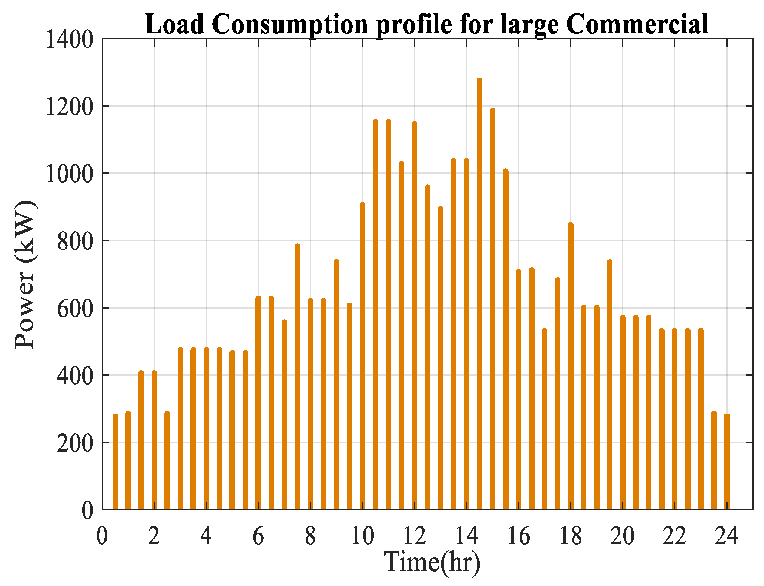
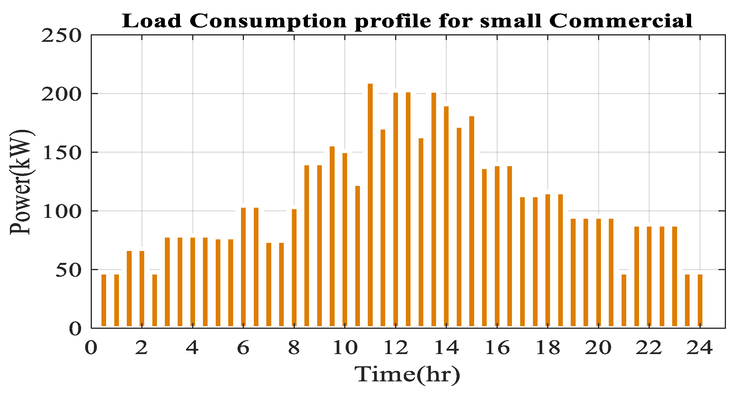
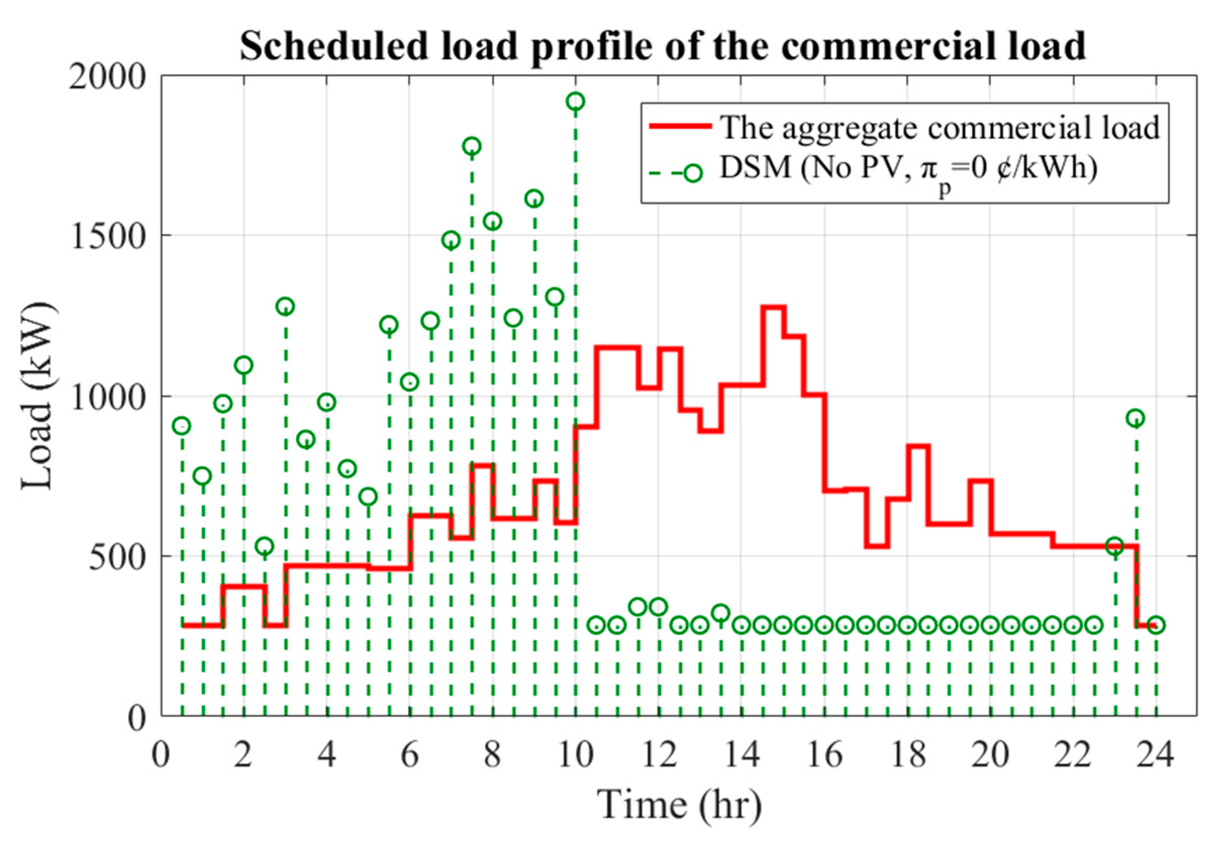
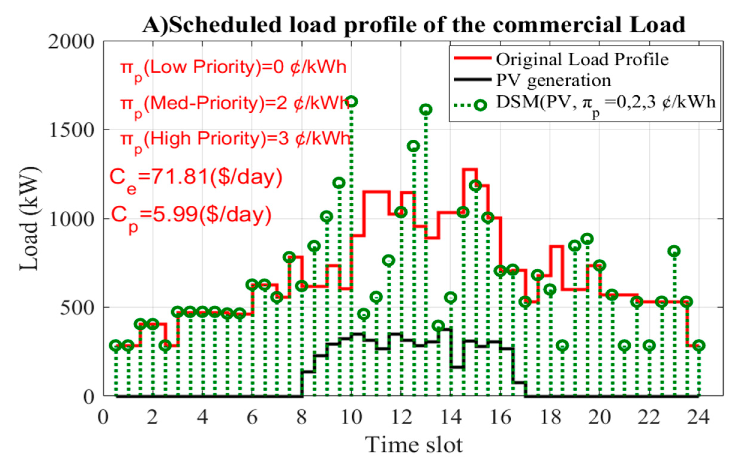
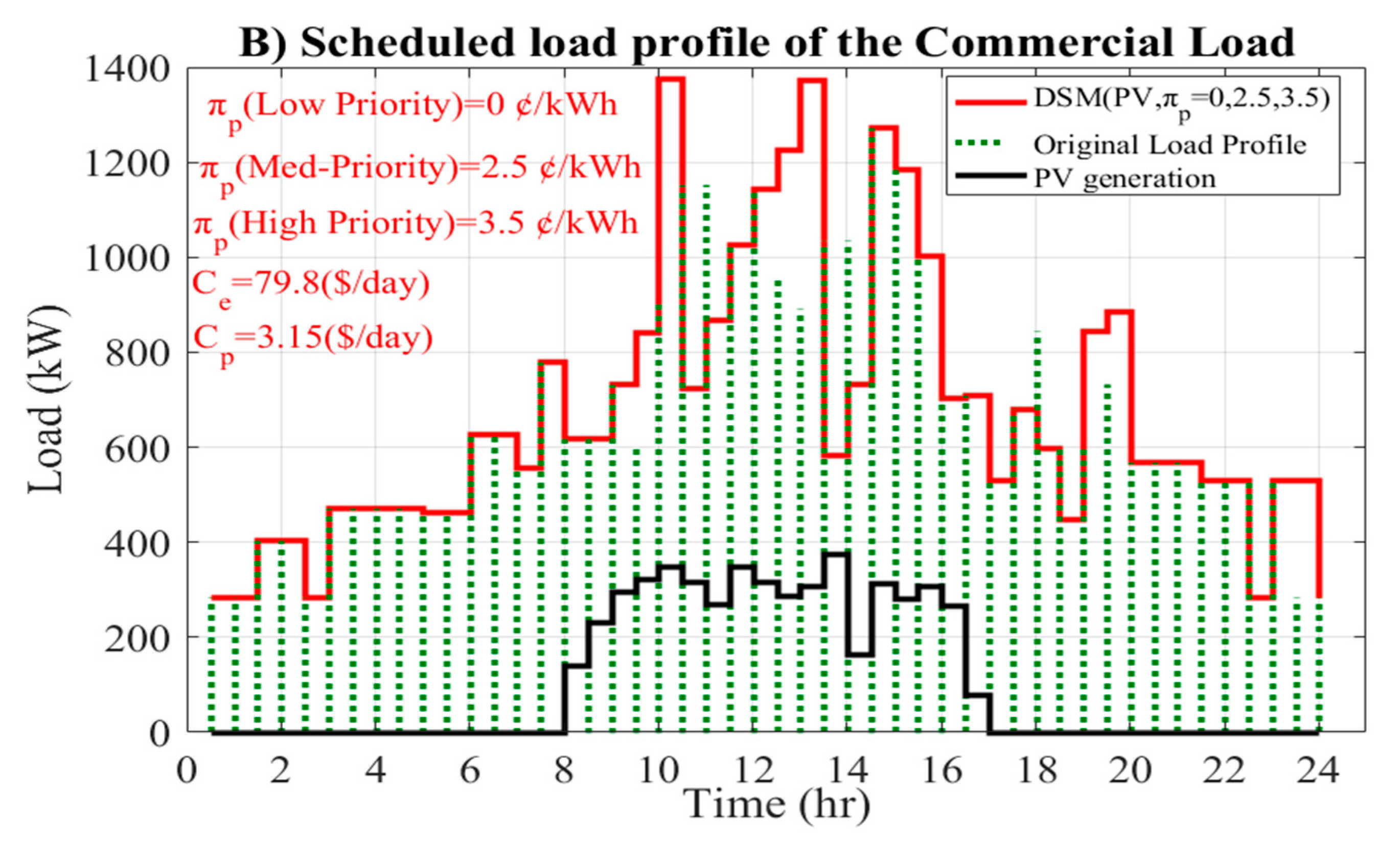
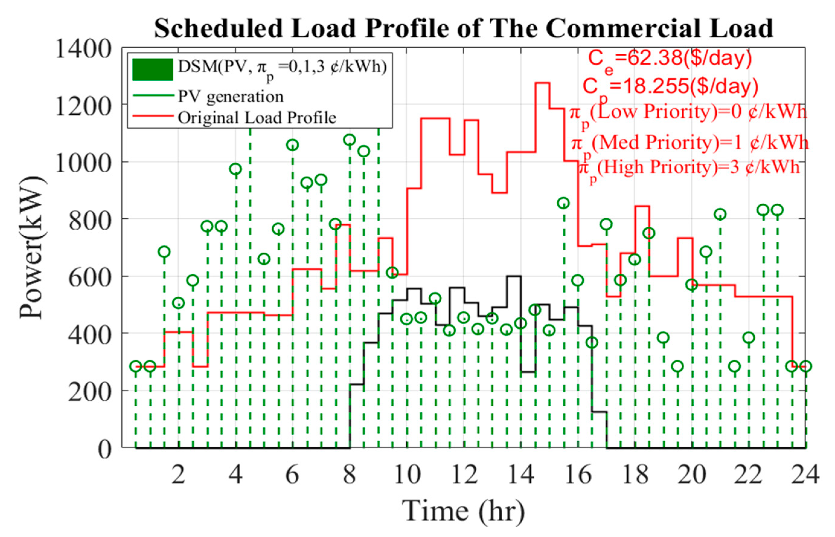
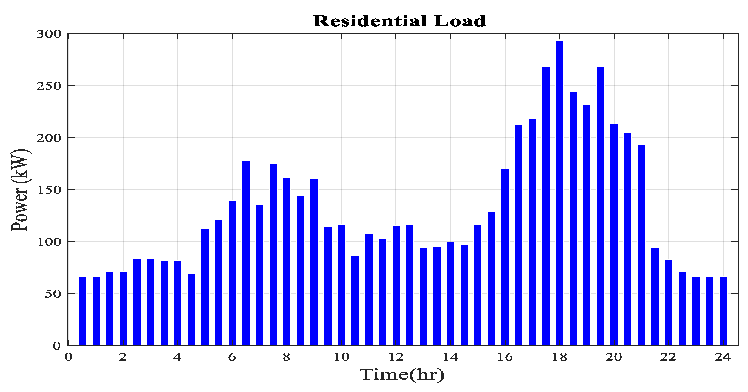
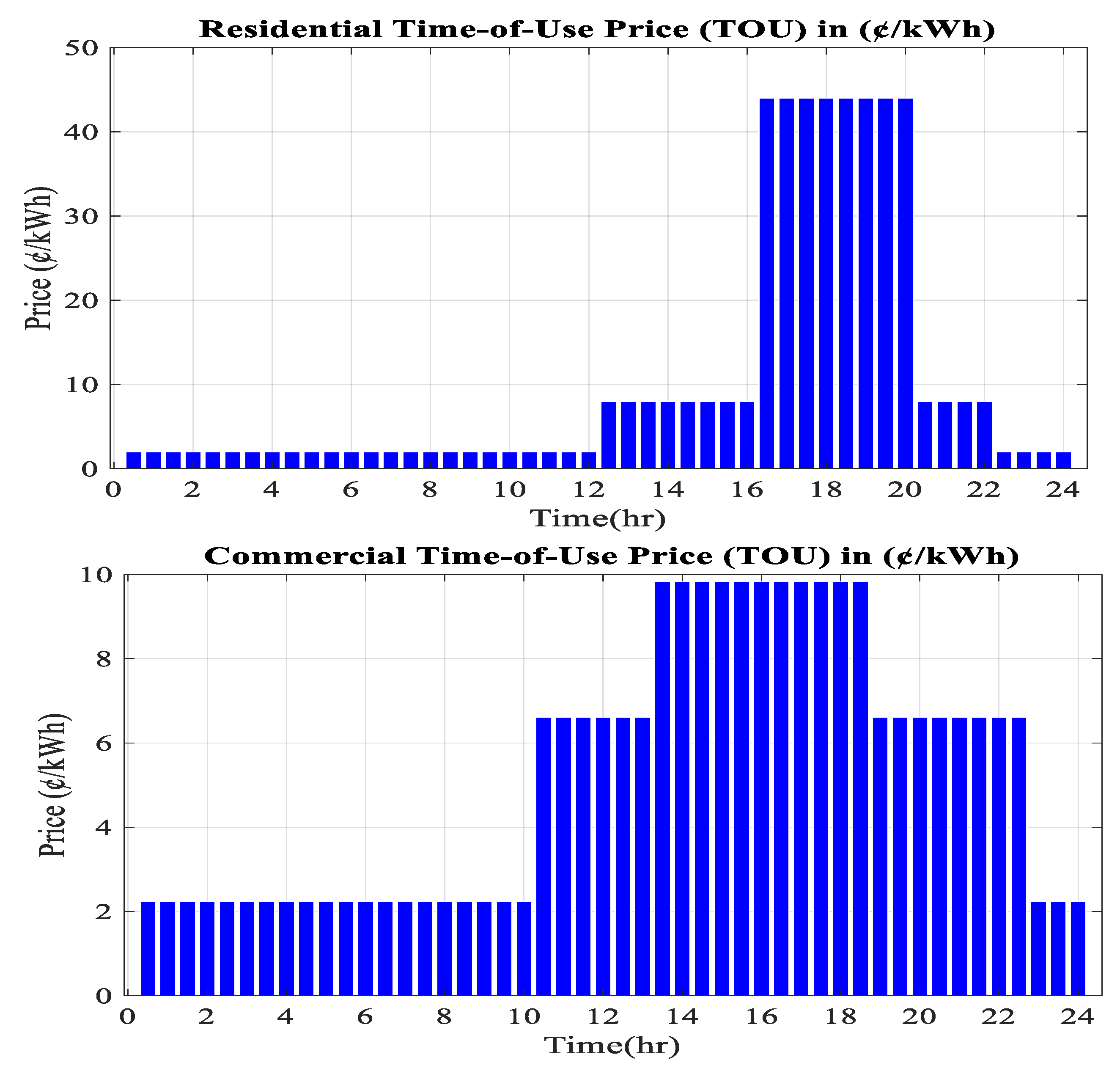
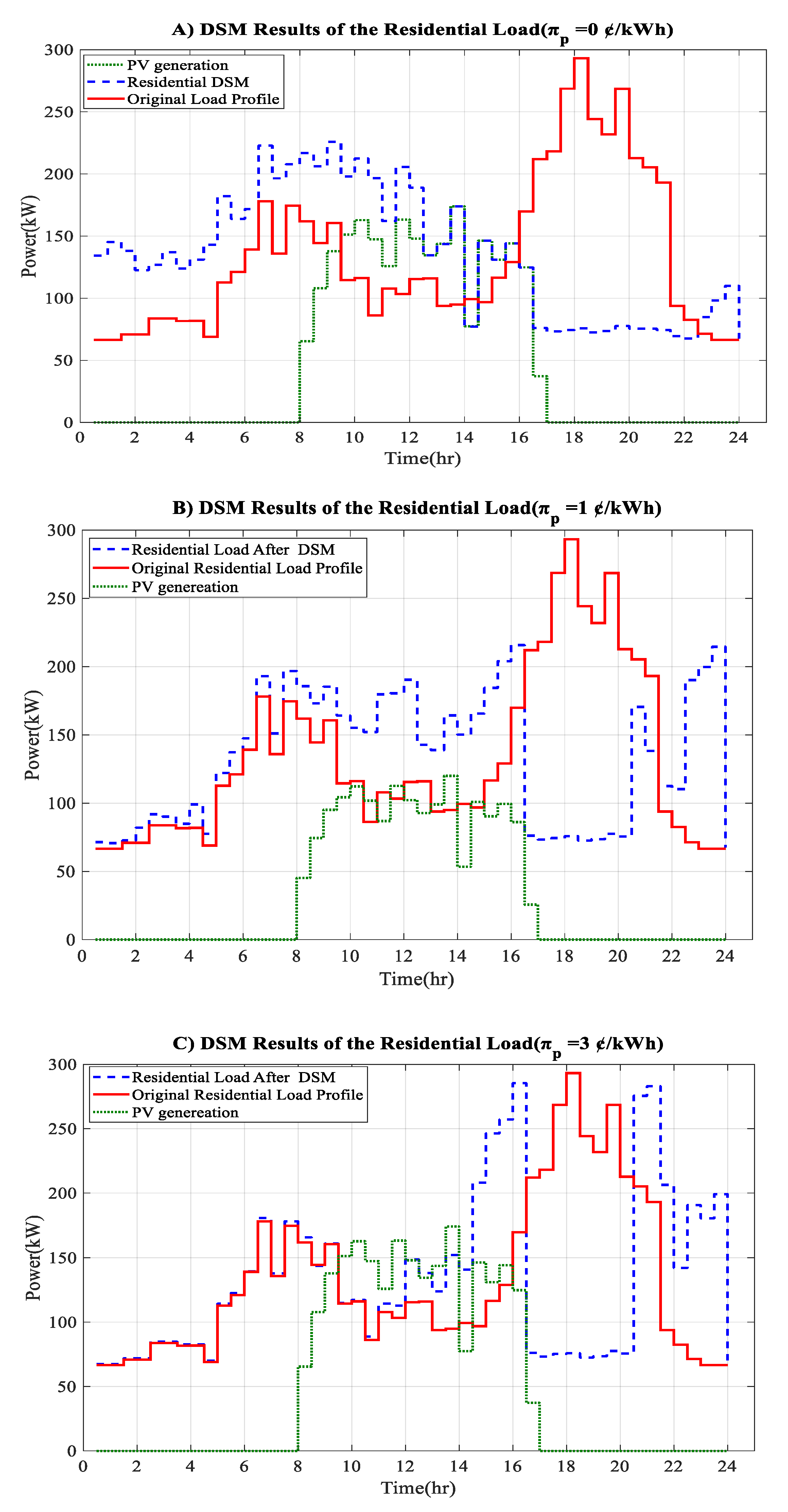
Figure 2 and Figure 3 show the curves for commercial activity. As shown in Figure 2 and Figure 3, high load appears between 9:30 a.m. and 5:30 p.m. Figure 4 illustrates the residential load profile, showing that most evening loads are subjected to peak electricity prices. In the commercial building (Bus No. 17), the appliance is scheduled based on the price provided in Figure 5 (commercial time of use pricing (TOU)). The four different types of appliances in the commercial building are shown in

Table A2. Appliances in the commercial area.

Categorization of Appliances	Index	Appliances	Operation Status	${\mathit{D}}_{\mathit{a}} \left(30\right)\min$	Power Rate (kW)
Baseline Appliances	1	Icebox	All day	48	22.5
	2	Lights	All day	48	240
	3	Closed-circuit television	All day	48	22.5
High Priority ${\pi }_p$ = 3 ¢/kWh	4	Welding device	15−19	5	109.5
	5	Electric fan	24−27	4	109.5
	6	Arc furnace	25−28	4	270
	7	Three0phase motor	21−24	3	270
	8	Direct current motor	22−24	3	270
	9	Ice machine	13−17	5	57
	10	Drum machine	7−11	5	189
	11	Broiler	21−24	4	189
	12	Drill	39−42	4	246
Medium Priority ${\pi }_p$ = 1 ¢/kWh	13	Pizza oven	43−46	4	189
	14	Food display	25−29	5	105
	15	Dispenser	20−24	5	111
	16	Laundry machine	30−34	5	96
	17	Sewing machine	40−44	5	240
	18	Microwave	16−20	5	285
	19	Frying pan	23−27	5	246
	20	Dishwasher machine	37−41	5	225
	21	Heaters	14−18	5	225
	22	Waste disposal	36−41	5	225
Low Priority ${\pi }_p$ = 0 ¢/kWh	23	Shawarma machine	37−41	5	165
	24	Liquid dispensers	29−33	5	300
	25	Washing machine	27−31	5	270
	26	Shawarma machine	24−28	5	37.5
	27	Bun grilling	36−40	5	150
	28	Air conditioner	20−23	4	180
	29	Barbecue grill	27−30	4	180
	30	Meat Slicer	10−13	4	180
	31	Dough Mixer	30−33	4	180

(Appendix A). The four types of commercial appliance include the high-priority appliances, medium-priority appliances, low-priority appliances, and the base appliances. High-priority appliances refer to the case when these appliances are more important and the customer has to use them at any time, and these appliances have a low participation level in the DSM program; therefore, the appliances in this type are subjected to high tariffs. In medium-priority appliances, the operation time will not be very necessary (the time can be delayed and shifted to another period); thus, a lower tariff is applied on these types of appliances. The low-priority appliance can be on/off at any time and, therefore, a low tariff is applied on these appliances. The base appliances have to be on all day, and no tariff is applied; these appliances cost a fixed price. In the decentralized DSM, we minimize the cost, and the algorithm, in this case, will obtain the optimal load schedule for each load individually, before using analysis to calculate voltage fluctuation and energy loss. In other words, each household will reschedule the daily load according to the time-of-use pricing tariff; the results are then compared to show its impact on the distribution network operation and renewable integration, in terms of the utilization efficiency of rooftop PV generation, voltage fluctuation, and real power loss. Each household has its own load profile and the DSM is applied to find the optimal load scheduling based on a day-ahead price. Clearly, this involves static data. The original load profile does not change, and the model tries searching for the optimum operation time slots for each appliance to avoid the peak load time and to minimize the cost. We firstly consider a micro-grid network, as shown in Figure 1, which contains a single distribution feeder line supplying a small community of 29 houses. Each of these houses has a typical time-varying load profile generated by a time series load model we built based on realistic residential customer load data obtained from an open-access database with a rooftop solar PV panel with a rated capacity of 6 kW. It is assumed that the smart home has a set of commonly used active appliances under a real-time pricing environment, and that the homeowner has access to day-ahead electricity rates and a day-ahead forecast of PV generation, while agreeing to participate in the DSM program to save on electricity bills with a controlled number of sacrifices. For the purpose of simplicity of analysis, 31 active appliances were categorized into three groups based on their operational features as follows: (1) interruptible appliances, referring to electric devices able to be switched on or off at any time during a day; (2) uninterruptible appliances, referring to electric devices that need to operate until finished once started; and (3) inflexible appliances, referring to appliances that are active for the entire simulation time (24 h). Each appliance is modeled using four parameters, $s_a,f_a, r_a$, and $D_a$, where [$s_a,f_a]$ defines the allowable operating time during which the appliance may be switched on, and $r_a$ and $D_a$ denote the power rating and the total number of operating time slots as requested, respectively.

3. Mathematical Formulation

This section describes the model applied for the household individually taking part in the demand-side management (DSM) program. This model will help the participant to decrease their electricity bill and avoid usage of the load during the time of high price. The consumer inconvenience is modeled by a penalty in the objective. This part represents an additional cost that will help avoid the unnecessary load shift. The optimization model is illustrated below.

$$\underset{[{\mathrm{u}}_{a,m}(\mathrm{t})]}{\min } C_e^m+C_p^m,$$

(1)

where $C_e^m$ refers to the energy usage cost, and $C_p^m$ is the total penalty cost ($/day) in household $\mathrm{m}$. The energy usage cost is subject to

$$C_e^m=0.5\times {{\displaystyle \sum }}_t^T{P}_{load}^m\left(t\right)\times {\pi }_e\left(t\right),$$

(2)

where $P_{load}^m\left(t\right)$ is the household load that needs to be optimized, ${\pi }_e\left(t\right)$ is the time-of-use pricing, T refers to the number of time slots (T = 48), and t is the time slot index.

$$C_p^m=0.5\times {{\displaystyle \sum }}_{a,m}^A{\pi }_p· r_{a,m}·\Delta T_{a,m},$$

(3)

where constraints in Equations (2) and (3) apply to the electricity and the penalty cost. In Equation (3), ${\pi }_p$ is the penalty price in cents (¢),$r_{a,m}$ is the power rate of appliance a in household m, and $\Delta T_{a,m}$ refers to the number of slots shifted after applying DSM.

$${P^m}_{load}\left(t\right)=\max (({{\displaystyle \sum }}_{a,m=1}^{A_m}{r}_{a,m}\times u_{a,m}\left(t\right)- \alpha ·{P^m}_{pv}\left(t\right)) , 0).$$

(4)

Equation (4) is applied to remove negative cost. For this model, it is assumed that surplus generated power from PV can be delivered into the grid with zero reward; therefore, the cost at each time slot should not be less than zero. In Equation (4), α is a binary parameter representing the status of PV installation at the DSM household, m is the home index,$u_{a,m}$ is the operation status of appliance a (0 when the appliance is off, and 1 when it is on), and ${P^m}_{pv}\left(t\right)$ refers to the power generated by the solar PV in household m.

$${{\displaystyle \sum }}_{a,m=1}^{A_m}{r}_{a,m}\times u_{a,m}\left(t\right)\le M{D}^m\hspace{1em}\hspace{1em}\hspace{1em}\forall a \in \left\{1 to A_m\right\}.$$

(5)

The maximum load to be used at each time slot is indicated in Equation (5). This load limit can help in the prevention of load peak even when the electricity price is low. Here, $M{D}^m$ refers to the threshold of usage.

$${{\displaystyle \sum }}_{t=1}^T{u}_{a,m}\left(t\right)=D_{a,m}\hspace{1em}\hspace{1em}\hspace{1em}\hspace{1em}\hspace{1em}\forall a \in \left\{1 to A_m \right\};$$

(6)

$$u_{a,m}\left(t\right)=0\hspace{1em}\hspace{1em}\hspace{1em}\hspace{1em}\hspace{1em}\hspace{1em}\hspace{1em}\forall t < s_{a,m }\mathrm{or}\forall t > f_{a,m }.$$

(7)

Constraints in Equations (6) and (7) define the total operation time status of an appliance. Here, $D_{a,m}$ is the time duration of each appliance, while $[s_{a,m }$,$f_{a,m}]$ represents the possible start and end time slot for each appliance.

$$\Delta T_{a,m}=1^T.\left|t_{a,m}^{s{t}_{new}}-t_{a,m}^{s{t}_{old}}\right|\hspace{1em}\hspace{1em}\hspace{1em}\forall a \in \left\{1 to A_m\right\}.$$

(8)

The constraint in Equation (8) indicates the number of time slots shifted by calculating the difference between the old slots and the new slots.

$$t_{a,m}^{s{t}_{new}}={\left[t|u_{a,m}^{new}\left(t\right)=1\right]}_{1\times D_{a,m}}\hspace{1em}\hspace{1em}\forall a \in \left\{1 to A_m\right\};$$

(9)

$$t_{a,m}^{s{t}_{old}}={\left[t|u_{a,m}^{old}\left(t\right)=1\right]}_{1\times D_{a,m}}\hspace{1em}\hspace{1em}\hspace{1em}\hspace{1em}\forall a \in \left\{1 to A_m\right\}.$$

(10)

Constraints in Equations (9) and (10) specify the old time slot before shifting and the new time slot after shifting ($t_{a,m}^{s{t}_{old}}$ and $t_{a,m}^{s{t}_{new}}$, respectively), which allows specifying the time duration of interruptible appliances.

$$\left[v\left(t\right)\right]=f_{AC}(P_g\left(t\right),P_g^{PV}\left(t\right), P_L^{*}\left(t\right)|Y_{bus}).$$

(11)

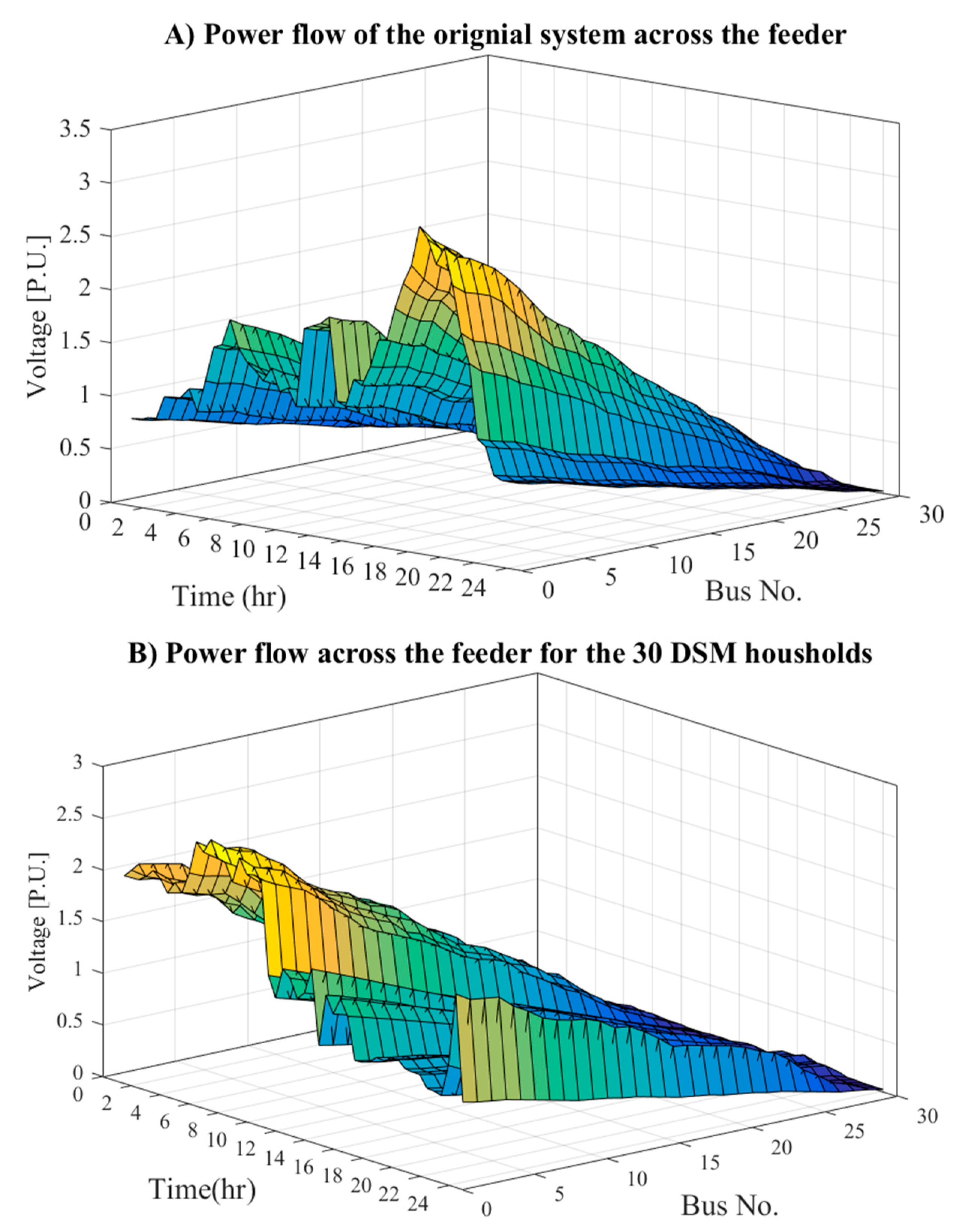
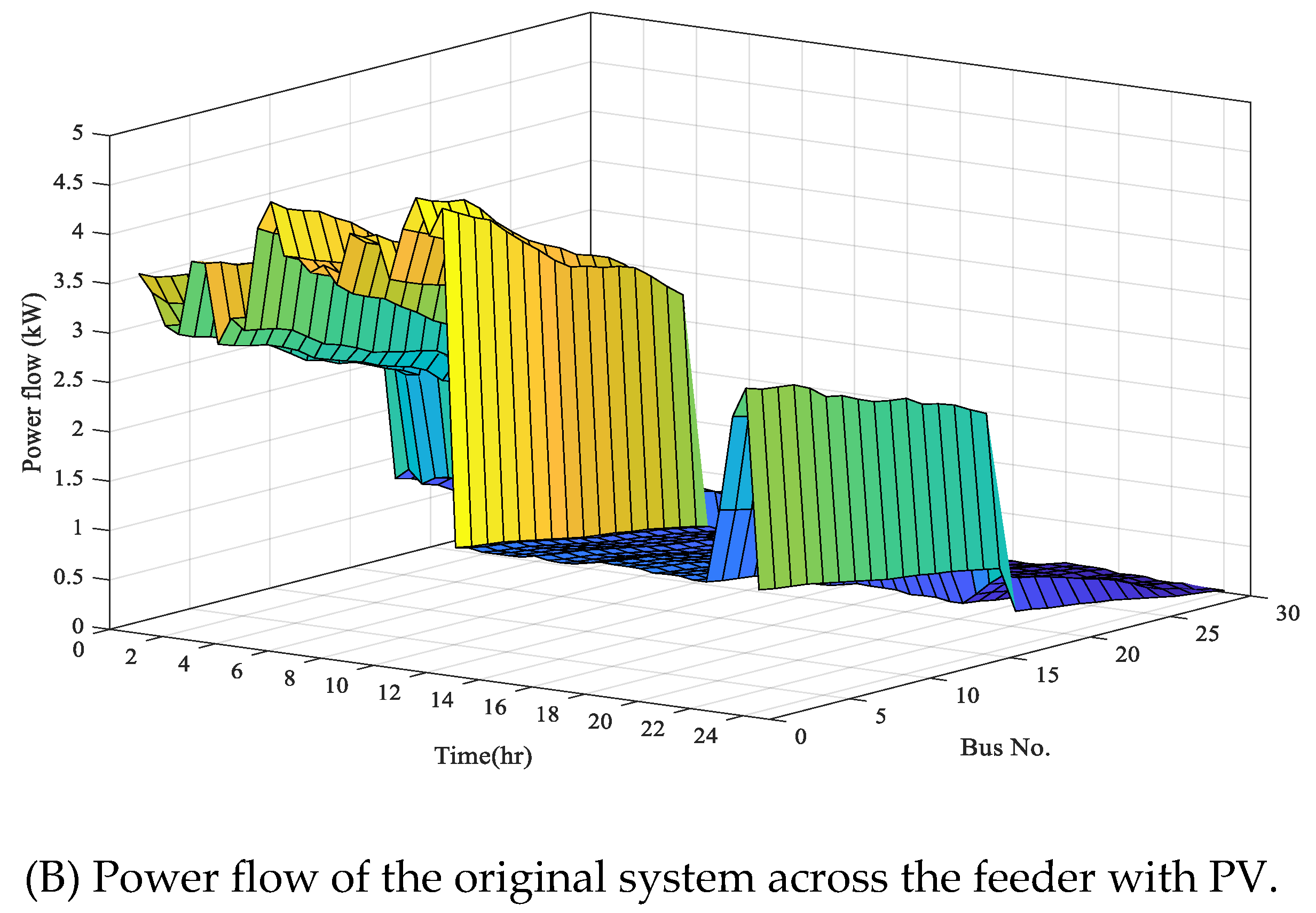
The constraint in Equation (11) is used for load flow calculation, where $P_g\left(t\right)$ represents the injected power from the substation, $P_g^{PV}\left(t\right)$ is the available PV generation, and $P_L^{*}\left(t\right)$ is the electrical load after DSM scheduling.

$$E_{loss}={{\displaystyle \sum }}_{t=1}^T{{\displaystyle \sum }}_{l=1}^L{\left|i_L^t\right|}^2{R}_L.$$

(12)

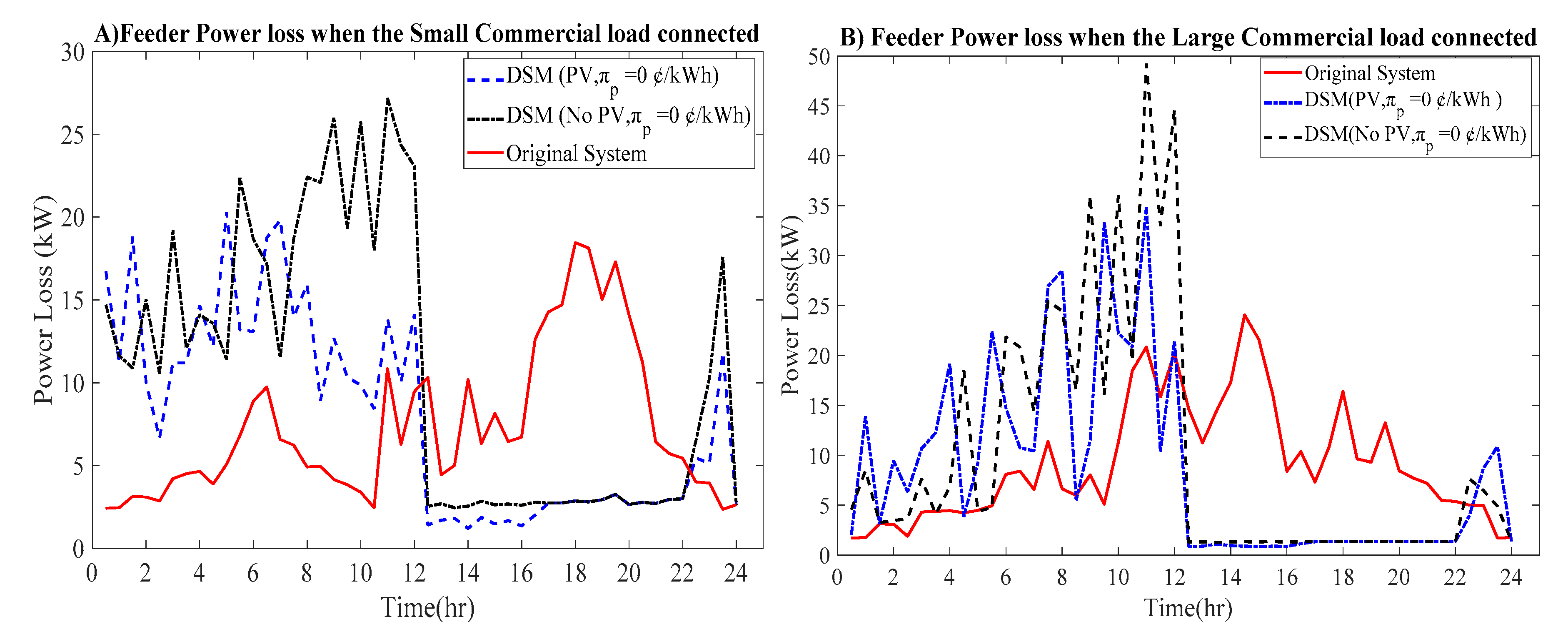
The constraint in Equation (12) is used to calculate the system power loss, where $i_L^t$ is the current of the feeder L at time t, and $R_L$ is the resistance of line L.

$${\sigma }_v=\sqrt{\frac{1}{T\times N}{{\displaystyle \sum }}_{t=1}^T{{\displaystyle \sum }}_{i=1}^N{\left(v_i^t-\overline{v}\right)}^2}.$$

(13)

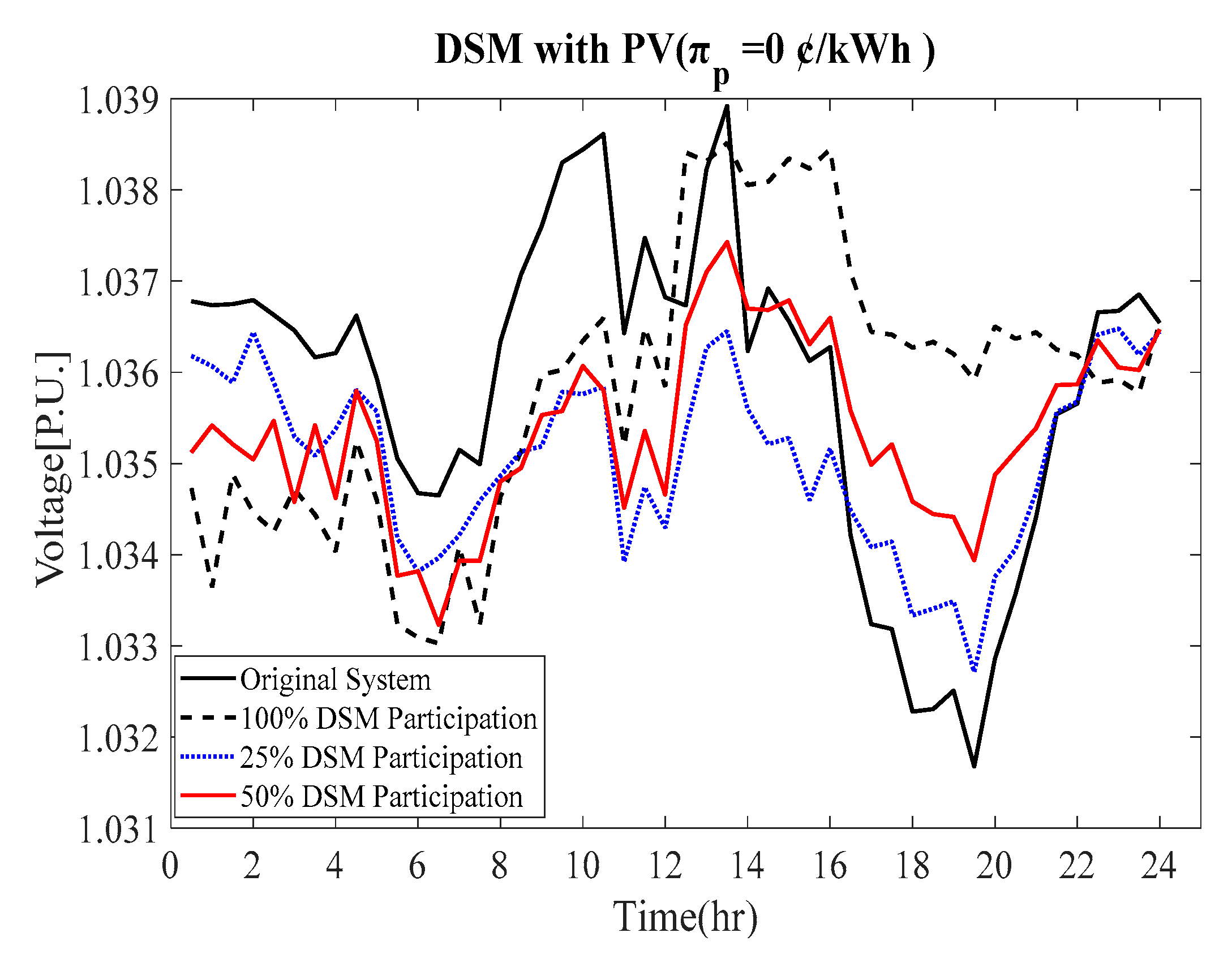
The constraint in Equation (13) defines the voltage fluctuation (${\sigma }_v$) index with $v_i^t$ as the voltage of bus i at time t, and $\overline{v}={\displaystyle \sum }_{t=1}^T{\displaystyle \sum }_{i=1}^N{v}_i^t$ as the average voltage in the network. Here, m is the home index, and $u_{a,m}$ is the operation status of appliance a (0 when the appliance is off, and 1 when it is on), with the following format:

$${[u_{a,m}\left(t\right)]}_{A\times T}=[u_1^1, u_1^2,\dots , u_1^T;u_2^1,u_2^2,\dots u_2^T;.....; u_A^1,u_A^2,...,u_A^T],$$

where T refers to the number of time slots (T = 48), and t is the time slot index. The household appliances were modeled using the measurable factors $s_a$,$f_a, r_a$, and $D_a$, where [$s_{am, }{f}_{a,m}$] are parameters defining the operating period when the household appliance a can be operated, and $r_{a,m}$ and $D_{a,m}$ represent the appliance power rating and time duration of the appliance.

Typically, when there is no shift, the penalty cost is zero ($C_p=0 \$/day$), which means no time slots are shifted for the operated appliances and $\Delta T_a= t_{a,m}^{s{t}_{new}}-t_{a,m}^{s{t}_{old}}=0$. In this case, the consumer has to pay for the consumed energy (kW/h) as electricity (${\mathcal{C}}_e)$ based on the TOUP. With optimal shifting, the total cost that the consumer has to pay will be reduced due to the cost saving ($C_{saving}$) in ¢/kWh, which comes after the shift in operation time from a high-price to a low-price period. In this case, the consumer will pay the extra cost as a penalty cost. It is important to mention that the algorithm allows a shift whenever cost saving is possible elsewhere ($C_{saving }>C_p$), and the total cost paid by the consumer is represented by ${\mathcal{C}}_e-C_{saving }+C_p$, where $C_{saving}$ is the cost saving, $C_p$ is the penalty cost, and ${\mathcal{C}}_e$ is the total electricity.

4. Simulation Results

To examine the impact of the decentralized DSM on the operation status of the grid (e.g., utilization efficiency of the energy generated by the PV, voltage fluctuation, system energy loss, and the reverse power flow), the DSM was firstly applied to some households with and without PV-generated power. Secondly, we studied the impact of different DSM penetration levels on the network performance.

4.1. DSM of the Residential Household Area

Figure 3 shows the difference between the preferred consumption (original load profile; solid line) and the aggregated load (dotted line) after applying the proposed DSM, with π_p = 0, 1, or 3 ¢/kWh. The preferred daily load consumption shows two high-load periods: around 6:30 to 8:00 a.m. and 4:30 to 7:30 p.m. The load during the evening is exposed to the time of high rate; hence, most of the flexible appliances tend to shift to a part of the day when the price is low (see Figure 6A). On the other hand, at penalty π_p = 1 or 3 ¢/kWh, we see a few appliances shift to off-peak load, as illustrated in Figure 6B,C. It is worth noting that, by increasing the penalty factor, the participation of uninterruptible appliances in load shifting is discouraged due to their constraint of continuous operation after starting. For rescheduling uninterruptible appliances, the DSM program needs to incorporate more time shifting and, most of the time, it imposes a larger penalty cost compared to the electricity cost saving. However, interruptible appliances with more flexibility to reschedule may actively participate in a DSM program with a penalty factor, because their operational feature allows them to be switched on or off at any time within the allowable operation time range.

4.2. DSM of the Commercial Area

Figure 7 shows that, when assuming π_p = 0 ¢/kWh, more of the load is moved into time slots with a low-price period. As stated in the introduction, for a more realistic scenario, the proposed algorithm also take into consideration the fact that certain appliances may have higher priority over other appliances such that these appliances have to operate in their specified time; hence, these types of appliances have less DSM participation. The obtained results for the commercial area are given in Figure 8 and Figure 9, with the comparison of the preferred load (original load consumption; solid line) and the new profile after applying the DSM (green dotted line), showing that there is only one high-load period from 9:30 a.m. to 4:30 p.m. Figure 10a illustrates the cost saving of the shifted appliances and the corresponding penalty cost for π_p = 0, 1, and 3 ¢/kWh, reporting the penalty prices applied for low-, medium-, and high-priority appliances, respectively. The obtained results show that one high-priority appliance participated in the DSM with one time slot shifts, while five appliances under the medium-priority category participated. It is worth noting that the corresponding cost saving depends not only on the reduced electricity price caused by the shifted time slots but also on the power rating $r_a$ of the appliance. Lastly, for the low-priority category, we can see that the number of appliances participating in the DSM increased to nine, with much higher cost saving and a higher number of shifted time slots. We can also see from Figure 10a that the low-priority appliances had zero penalty cost (π_p = 0 ¢/kWh). Figure 11 and Figure 12 illustrate the cost saving for the appliances and their corresponding penalty cost from the time slots shifting across two different values for the medium-priority category. Also, from Figure 10, we can see that appliance No. 30 appears, and the reason is that the appliance operated originally in the time slot with a low electricity price; thus, it will not shift unless there will be cost saving. In other words, if the cost saving resulting from time shifting becomes lower than the corresponding penalty cost, then the suggested time shift will be rejected.

4.3. Comparison of Experimental Results

4.3.1. Electricity Cost

The results show that the daily cost of the residential households was reduced from a total value of $417.74 to $261.76. With the DSM, the results show a cost reduction of 38.1%. The results for the commercial area are summarized in Figure 9, whereby the cost of the commercial building was reduced from $88.22 to $43.27 (50.4%). The impact of demand side management on the cost summarized in

Table 1. Impact of demand-side management (DSM) on the daily cost.

Type of Load	Original Cost without DSM ($)	Cost after Applying DSM ($)	Percentage Reduction
Residential household load	417.74	261.76	38.1%
Commercial load	88.22	43.27	50.4%

.

Typically, DSM shows better improvement of the results when more flexible appliances are available for shifting. However, even when the number of flexible appliances was lower (e.g., in the commercial load), the percentage reduction in the electricity cost was higher than that in the residential load. Also, the residential load had a higher number of rescheduled appliances, but the percentage cost reduction was lower than that in the commercial load. This was due to the higher power rate of the appliances in the commercial load in comparison with the much lower power rate of the appliances in the residential area. Additionally, when some appliances were moved to another time slot, it resulted in big savings for the user.

4.3.2. Solar PV Usage Efficiency

The efficiency of solar PV usage is defined as the total PV power consumed with respect to the total energy generated from the solar PV. The results show the effect of applying a high penalty on the efficiency of solar PV usage. The efficiency of usage dropped in the case of residential loads when π_p = 3 ¢/kWh, where the utilization efficiency was 89%. In fact, applying a high penalty added more restriction on appliances with regard to shifting to a time power was generated by the solar PV; as a consequence, the solar PV usage efficiency was reduced. The efficiency of usage was 92% in the commercial buildings because the entire PV-generated power was consumed in the period of peak load demand.

4.3.3. Real Power Loss

Figure 13 compares the feeder’s real power loss in terms of residential and commercial DSM. The feeder’s power loss was 738.36 kW and dropped to 314.27 kW (56.85%) for the commercial are. For the residential area, the loss dropped to 522.54 kW (28.25%). PV solar panels with a rated capacity of 6 kW were used for the residential area in our model, and a capacity of 600 kW was used for the commercial area. Although the residential load had the highest number of appliances available for rescheduling, it is obvious that applying the DSM on commercial loads was more effective, because the appliances (e.g., dough mixer, bun-grilling toasters, and gyro machine) had a higher kW rating. The rescheduling of these appliances to the time of PV power generation tended to reduce line loss much better.

4.3.4. Voltage Profile

When applying a DSM model, it is necessary to ensure no voltage violation (a value greater than 1.04 P.U.) Where P.U. is a per-unit. Figure 14 clarifies the voltage deviation of Bus No.17 for the small commercial load. There is a clear difference between the profiles with and without solar PV, especially between 12:30 p.m. and 4:00 p.m., as most of the demanded load was covered by the PV-generated power. The increased voltage was caused by the reverse power flow, which can be curbed by reducing the active power injected from the solar PV. In this work, voltage increased during the low-consumption time slots with PV generation at the maximum level. A possible solution for this voltage rise can involve either reducing the network resistance or reducing the PV power penetration level during the simulation. As shown in Figure 14, a two-fold reduction in power penetration level caused a slight reduction in voltage level.

4.3.5. Real Power Loss at ${\pi }_p$ = 0 ¢/kWh

From Figure 15, it is clear that the power loss decreased upon injecting PV-generated power. As we can see, between 8:00 a.m. and 12:30 p.m., the power loss was reduced. The overall reduction in power loss was 26%. As shown in Figure 15A with the black dotted line, for the case of the DSM (no PV, π_p = 0 ¢/kWh), there was an increase in the power loss between 8:00 a.m. and 12:00 p.m., as the load demand at this time was high, as was the current drawn from the grid. The blue dotted line shows the feeder power loss in the presence of solar PV generation. In the time from 8:00 a.m. to 12:00 p.m., the power loss showed a significant reduction, because both of the loads consumed the power from the solar PV and, consequently, the current was reduced.

Table 2. Photovoltaic (PV) utilization efficiency at different penalty prices (${\pi }_p$).

PV Utilization Efficiency
Penalty Price πp (¢/kWh)	Residential Area	Penalty Price πp (¢/kWh)	Commercial Area
0	98%	0	98%
5	72.3%	2	100%
10	64.8%	3	100%
20	58.4%	5	100%

summarizes the effectiveness of considering a high tariff on the efficiency of solar PV usage. It shows that the efficiency of solar PV usage dropped for the residential area, while it increased for the commercial building, where the highest PV-generated power occurred at the period of peak commercial load (see Figure 2 and Figure 3). The feeder power loss calculation is given below.

$$P_{Loss}={\displaystyle \sum }_{i=1}^{ n_{br}}{\left|I_i\right|}^2 r_i,$$

where $n_{br}$ is the number of nodes in the feeder, $\left|I_i\right|$ is the node current of i, and $r_i$ is the resistance.

4.3.6. Reverse Power Flow

Figure 16 presents the power flow distribution across the distribution feeder for the original system without DSM, and with all the residential households participating in the DSM (${\pi }_p=0$ ¢/kWh). DSM participation helped smooth the flow of distributions along the feeder and, hence, no reverse power flow occurred. Figure 17 illustrates the power flow distribution across the distribution feeder with DSM (with PV, ${\pi }_p=0$ ¢/kWh), meaning all customers had PV generation installed. Reverse power occurred at the time with high PV power penetration levels to the bus while the load demand was at its lowest level, which can also cause a voltage rise. As shown in Figure 17A, reverse power occurred during the time slots at which the PV generation was at a maximum level while the load demand was at a minimum level. Figure 17B shows that, when the DSM is applied, more appliances were rescheduled and shifted to the time when energy was generated by the solar PV, which helped remove the reverse power flow.

4.4. Desterilized DSM Comparison for Different Participation Levels

Figure 18 compares the feeder voltage for different participation levels with πp= 0 ¢/kWh, considering two scenarios (i.e., with or without PV installation). It can be seen that increasing the number of customers participating in DSM will tend to smooth the voltage profile and decrease the voltage fluctuation caused by load changes. Moreover, when the rooftop PV energy generation was at the highest level (8:30 a.m. to 4:30 p.m.), the DSM at π_p = 0 ¢/kWh helped mitigate the voltage rise during these hours. Figure 19 illustrates the feeder total power loss with varying number of customers with the presence of a rooftop PV. As we can see, with higher DSM participation (note that, in this case, 100% means all 30 customers participated in the DSM program), the power loss is reduced with the on-peak price, as illustrated in

Table 3. Feeder power loss in kW for different participation levels.

The Applied Scenario	100% DSM	50% DSM	25% DSM
DSM with PV	136.5	153.6	172.5
DSM without PV	202.63	199.97	197.33

. As depicted in Figure 20, with DSM (at penalty π_p = 0 ¢/kWh), more loads were rescheduled to the free power time (solar PV generation) at midday, which mitigated the real power loss. Lastly, the voltage profiles at the end of the feeder with 30 smart homes participating in the decentralized DSM program were compared. As this test was applied at different values of penalties with the presence of rooftop PV, when the value of πp increased from 5 to 10 ¢/kWh, the voltage became less flattened, and only the flexible (less preferred) appliances were rescheduled to the time when the solar PV panel had maximum generation (Figure 20).

5. Conclusions

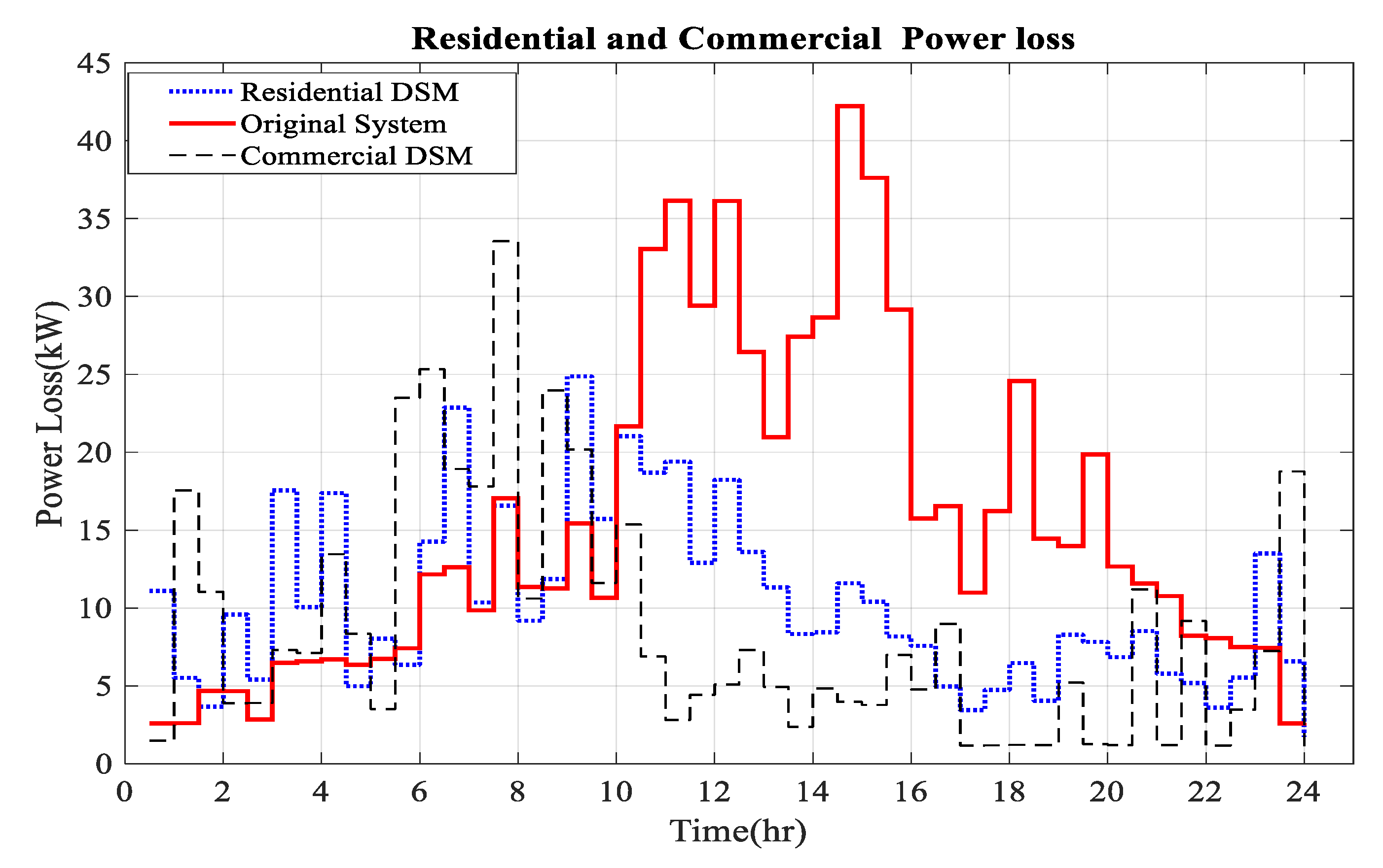
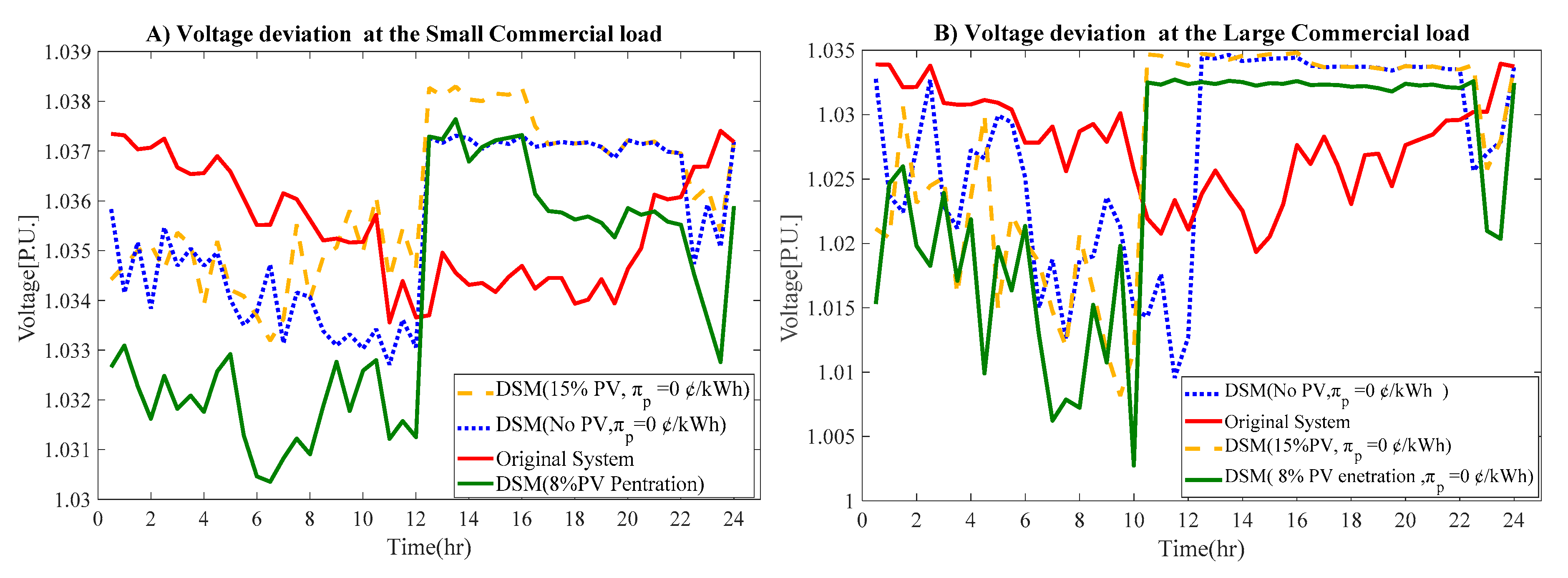
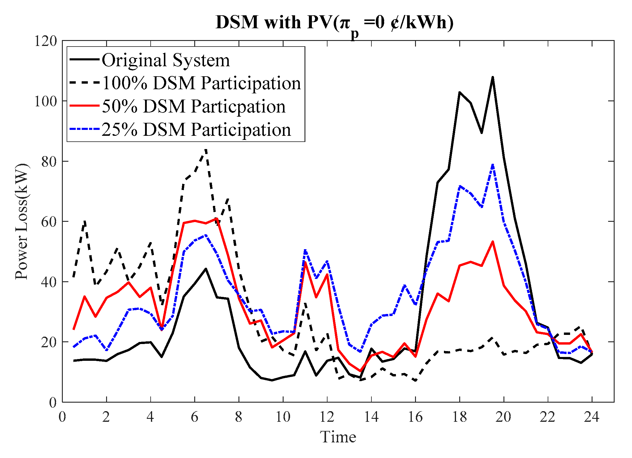
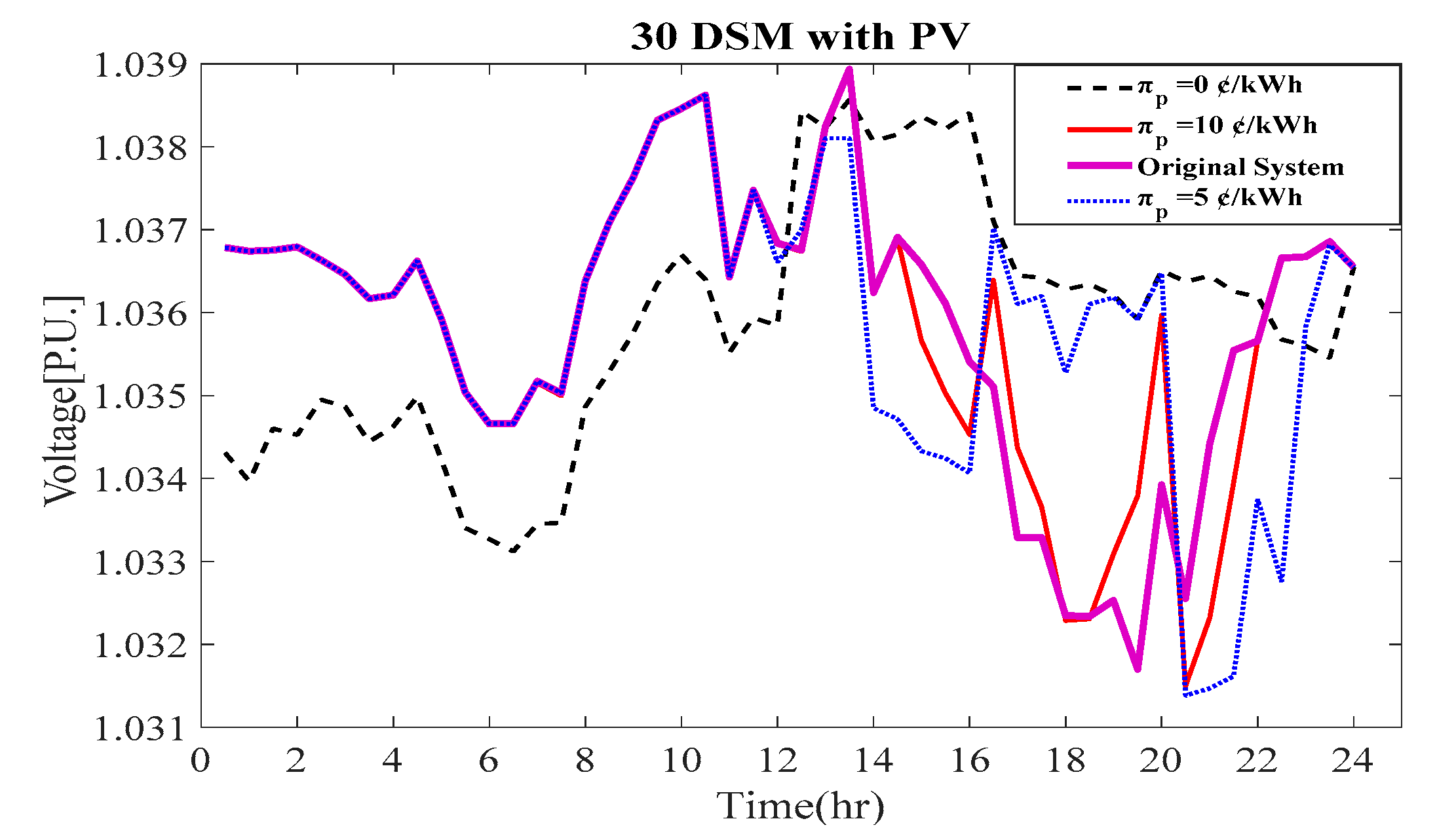
In a radial distribution network of 30 buses, we examined the following: (1) electricity cost, (2) efficiency of solar PV usage, (3) line power loss, and (4) voltage fluctuation (${\mathsf{\sigma }}_{\mathrm{v}}$ in P.U.). From the results, it is clear that the commercial DSM showed better effectiveness than the residential DSM, with reductions in electricity cost of 50.3% and 37.1%, respectively, due to the high power rate of the appliances in the commercial load, meaning that any small shift resulted in much higher savings than with residential appliances. Also, the commercial load profile showed a time alignment with local solar insolation and, thus, PV generation; therefore, the commercial DSM exhibited better electricity cost savings, higher efficiency of solar PV usage, a larger decrease in electric energy loss, and better improvement of voltage fluctuation. In addition, the overall simulation illustrated that the decentralized DSM had a negative effect on grid energy loss. Thus, it is necessary in the future to adopt coordinated DSM optimization for commercial loads to see how it affects system performance.