Multi-Objective Optimal Cloud Model Design of Vehicle-to-Grid Connected Systems Based on the Multiple Performance Characteristic Index Method ^†

Abstract

In this paper, a statistical cloud model was proposed for optimal design of the proportional integral derivative (PID) controllers used in current control of vehicle-to-grid connected inverter systems with PID parameters. By collecting the effective control factors and noise factors from a cloud data base, the cloud model can minimize both the reactive power and the total harmonic distortion for the single-phase full-bridge vehicle-to-grid connected system. The multi-objective optimal solution is obtained by using statistical fuzzy-based response surface methodology with multiple performance characteristics index. The testing results showed the validity of the proposed cloud model. It is verified that the statistical cloud model can increase the performance of the single-phase full-bridge vehicle-to-grid connected system in practical vehicle-to-grid applications in the Internet of Things.

1. Introduction

The vehicle-to-grid optimization problem is currently very important for the power grid system. Therefore, an effective statistical model is proposed in this paper to meet the requirements of recent IOT applications. The smart power grid system should have Internet connections with cloud servers to provide useful information for the vehicle-to-grid inverter controller. When the vehicle joins the power grid system and supplies power into the grid, the power quality conditions can be fulfilled. The proportional integral derivative (PID) controller parameters of the vehicle-to-grid inverter can be specified. The total harmonic distorsion (THD) value and reactive power value are satisfactory by referring to the PID parameters suggested from cloud server.

In recent years, plug-in hybrid electric vehicles (PHEVs) have drawn great attention for clean energy applications. To make use of the battery storage coming from the hybrid electric vehicle, vehicle-to-grid connected power inverters were developed to provide the energy connection between hybrid electric vehicles and the power grid system.

There are two power connection types: one is three-phase type, and the other is single-phase type. In this paper, a single-phase vehicle-to-grid connected inverter was developed based on 110 V AC [1,2]. The DC voltage can be inverted into AC inverter voltage by a grid-connection inverter. Then, the AC inverter voltage is tied to the power grid system. Two control objectives are considered in this optimization problem. The first one is to minimize reactive power and the second one is to minimize the THD. The reactive power can be minimized under specific control [3]. Also, the THD value can be minimized by using specific current control [4].

In a power grid system, hybrid EVs and EVs might be located anywhere. Distributed loads might occur in any nodal point of the power grid. Grid connection problems might occur anywhere in the power grid system. The power quality problem of the grid is very important. The THD value should be very small to avoid current harmonics. Reactive power should be minimized to avoid transmission losses in the power grid system. The PID controller of grid connection plays a very important role in the two aspects. To final a suitable parameter set for PID controllers is essential. Different loading conditions might also affect the operation of PID controllers.

In References [1,2,3,4], the grid-connection problems related to THD values and reactive power values are explained. The power inverter control function has an effect on the THD value and reactive power value. In [1], the power quality related to the electric components of PV inverters was discussed. This revealed that the electric components had a relation with the power quality.

Therefore, two noise factors which are related to electric components are also discussed. In [2], the PLL controller discussed was also a PID-like controller. The parameters of the PLL controller affected the THD value. Therefore, the PID parameters are selected as control factors in the response surface model.

In [3], the reactive power related to active filters was discussed. The active filter was actually quite similar to a grid-connection inverter. The controller design was focused and the design of controller parameters was discussed. In [4], the anti-islanding problem of grid-connection inverters was discussed. The design purpose was to minimize the THD value. This revealed that the grid-connection inverter design had a relation with THD value.

Recently, the Internet of Things (IOT) concept is drawing great attention in many technical fields. The essential control factors and noise factors are transmitted and collected from electric vehicles equipped with internet modules in a cloud server. With the help of a cloud data base and a cloud model, smart optimal designs can be analyzed and determined by the cloud server. The associated collected cloud data are analyzed by the statistical cloud model to provide better system performance. In this paper, a statistical cloud model to help the controller design of the electric vehicle connections to the power grid system is discussed. The parameter design of the PID controllers for electric vehicles can be suggested and provided by the cloud server to ensure the power quality of the reactive power and THD value. This is helpful for the power grid system to ensure optimal operation and better power quality.

2. Principle of Vehicle-to-Grid Connected System Characteristics

The full-bridge type is selected in the single-phase inverter, as shown in Figure 1. Under the same output voltage V_uv, a smaller DC source value in the full-bridge type is required as compared with the half-bridge type. Therefore, only a smaller voltage rating of the electronic components is required and smaller volume and weight inverter design objectives can be achieved [5].

In practical industrial applications, PIDs are often and commonly used, so it is worthwhile to discuss the practical conditions of PID controllers. A PID controller requires some manual empirical laws to improve its performance. In this paper, a statistical model is proposed to develop the cloud model, achieve smart power grid applications and avoid manual empirical laws. This is the main advantage of the proposed model.

In the vehicle-to-grid connected inverter system, two closed PID control loops are used. The first one is the outer loop of the DC voltage V_dc coming from battery packs in the electric vehicle. The second one is the inner loop of the current I_grid flowing into the power grid system.

To simplify the analysis, the DC voltage source is assumed to be fixed in this paper and only the inner current loop is discussed. The PID controller standard form for the current loop can be formulated as shown in Figure 2 [6]:

$$u(t)=K_p·e(t)+K_i·{\displaystyle {\int }_0^{t}e(t)dt}+K_d·\frac{de(t)}{dt}$$

(1)

The transfer function is:

$$G_c(s)=(K_p+\frac{K_i}{s}+K_{d}s)=K_p(1+\frac{1}{T_{i}s}+T_{d}s)$$

(2)

where the e(t) is the input related to the system error. The term u(t) is the control output variable. K_p is the proportional gain. K_i is the integral gain. K_d is the derivative gain. T_is is the integral time constant. T_ds is the derivative time constant.

PID controllers are simple, low cost and easy to maintain. Both voltage control and current control are required in the proposed controller. There are many design methods for the conventional PID controllers such as Cohen-Coon and Ziegler-Nichols methods [7]. The Bode method is also popular in the control design area. However, the environmental noise factors may lead to some practical operation problems, and the optimal PID controller may not work perfectly well.

If the parameters of the PID controller are designed by only trial and error, the performance of the PID controller may not be optimal. In this paper, the design objective for the PID controller is to provide an optimal parameter set for the PID controller. A statistical method is considered in this paper. The essential control factors are considered and environmental noise factors are included. The optimal PID parameter set can be determined to overcome the practical operation problems.

3. Initial Design of a Single-Phase Full-Bridge Vehicle-to-Grid Connected System

In this paper, simulation software is used to simulate the vehicle-to-grid connected system first. By connecting the provided functional blocks in the software, the single-phase full-bridge vehicle-to-grid connected system is built up and simulated. Figure 3 shows block diagram used to represent a single-phase full-bridge vehicle-to-grid connected system. The DC voltage is used to represent the power source coming from the vehicle’s battery packs.

By using the full-bridge inverter, the DC voltage is inverted into AC voltage which is used to connect to the power grid system through the LC filter. For the current control loop, a specific current command is given to control the current flowing to the power grid. The output grid current is used as the feedback variable for the PID controller in the vehicle-to-grid connected inverter.

By using a PID controller, the output variable is used to provide the SPWM gate signals to control the power transistors in the power stage. The THD and reactive power are plotted as shown in Figure 4a,b. However, the THD and reactive power may not be in optimal conditions in the initial design stage.

Due to the space limitations, a description of the software simulation details cannot be fully proviided in this article. To verify its validity, the major key variables can be observed through a simulation. The major key problems—the total harmonic distortion (THD) and reactive power values—are shown in figures. It also shows that the THD value and reactive power value are related to the PID parameters.

Section 3 describes the software simulation. Therefore, some assumptions are required to complete the simulation. Figure 3 and Figure 4 are shown to verify the validity of simulation model. The simulation model is proved to show that PID parameters can affect the THD and reactive power values. Therefore, a statistical model formulation for this problem is proposed in this paper.

The single-phase full-bridge vehicle-to-grid connected inverter is connected to a power grid system with 110 V AC voltage. For power quality considerations, both the THD value and reactive power are expected as small as possible. A further experimental design with minimization problem is considered in the following sections. The optimization problem is formulated by using the response surface method with a fuzzy-based multiple performance characteristics index (MPCI).

4. Cloud Model Formulation for Optimal Controller Design

When the electric vehicle is connected in the power grid system, the electricity characteristics should be specified to ensure the power grid quality. Therefore, the THD value and reactive power value should be controlled. In the vehicle-to-grid problem, the vehicle supplies electric power into the power grid. To ensure the power grid quality, the PID controller information related to each power inverter should be clearly understood. Therefore, a cloud model is suggested to collect the PID parameters through a statistical model.

When each electric vehicle tries to connect into the power grid, the PID information can be provided by the cloud server through the Internet. The smart electric vehicle can access the PID information from the cloud server. The quality of grid connection can be ensured and a smart power grid application is achieved.

IOT technology has recently spread widely and rapidly in many technical fields. The optimal cloud model is considered to optimize the vehicle-to-grid interaction. By collecting data coming from electric vehicles equipped with internet modules, the essential control factors are recorded and collected in a cloud data base. A suitable cloud model is then required to analyze the optimal design for the collected control factors. In order to apply the response surface method [8] and fuzzy inference process [9,10], the following formulations are described.

4.1. Control Factors and Noise Factors for Selection of Cloud Data

This section describes the control factors and noise factors which are required for the response surface method (RSM). The control factors and noise factors have a relation with the output performance of the grid connection inverter. The smart grid connection inverter has automatic smart PID setting function from the cloud server through an Internet connection. Manual empirical setting of PID parameters is not required. This is an advantage of the proposed system. The electric vehicle can access the PID information from the cloud server and manual empirical settings can be avoided to ensure the power grid system quality.

When designing the vehicle-to-grid connected inverter, two design objectives are expected to be as small as possible. One is reactive power, and the other one is THD. The reactive power Q = VIsinθ. In order to make the power factor to be 1.0, cosθ = 1.0 and sinθ = 0.0. When sinθ = 0.0, the reactive power is ideally zero. The other one is thenTHD value. For a perfect current waveform, the THD value is ideally zero. The two design objectives must be minimized at the same time.

For the proposed method, three control factors are selected to be studied: K_p, K_i and K_d, as shown in

Table 1. Collected cloud data for control factors and corresponding levels.

	Level	Level 1	Level 2	Level 3
Factor
Control factor A, Kp		12,767	32,767	52,767
Control factor B, Ki		367	567	767
Control factor C, Kd		1 × 10−5	1 × 10−6	1 × 10−7
Noise factor 1, ESR (Ω)		2 × 10−10	4 × 10−10	6 × 10−10
Noise factor 2, rL (Ω)		1 × 10−6	3 × 10−6	5 × 10−6

. Since any temperature rise may affect the resistor value when the system is operating, for the response method, two noise factors should be selected for study: ESR and r_L. ESR is the stray resistance of the capacitor and r_L is the stray resistance of the inductor.

The “level” is the basic definition of the response surface method. Three level values should be setup first to fit the response surface method. The response surface method is widely used in the technical statistics area. The response surface method has many standard combinational tables for practical applications. One of the standard tables is sixteen experimental runs with four central-point experiments. This is a standard table response surface method.

In the response surface method, the experimental runs are different from the central-point experiments. Therefore, the level settings for the control factors and noise factors are different. In response surface basic theory, there are clear description of these questions. Due to space limitations, a detailed description of the response surface method cannot be included in this paper.

4.2. Cloud Model Design by Using Combined Array Method

In the design of experiments, there are sixteen experimental runs should be measured first as shown in

Table 2. Combined array collected from the cloud data base.

Run	Kp	Ki	Kd	ESR (Ω)	rL (Ω)
1	−1	−1	−1	−1	1
2	1	−1	−1	−1	−1
3	−1	1	−1	−1	−1
4	1	1	−1	−1	1
5	−1	−1	1	−1	−1
6	1	−1	1	−1	1
7	−1	1	1	−1	1
8	1	1	1	−1	−1
9	−1	−1	−1	1	−1
10	1	−1	−1	1	1
11	−1	1	−1	1	1
12	1	1	−1	1	−1
13	−1	−1	1	1	1
14	1	−1	1	1	−1
15	−1	1	1	1	−1
16	1	1	1	1	1

. Four central-point experiments are also required to assess the curvature of the measured data as shown in

Table 3. Central point data collected from the cloud data base.

Run	Kp	Ki	Kd	ESR (Ω)	rL (Ω)
1	0	0	0	0	0
2	0	0	0	0	0
3	0	0	0	0	0
4	0	0	0	0	0

.

4.3. The Fuzzy Inference with MPCI in Cloud Model

The MPCI method is used to derive the multiple-objective functions. The two objective functions are integrated into one compact value. This means the derivation of MPCI value is equal to the solution of the multiple-objective optimization problem. The derived optimal PID parameters can be suitable for both objective functions, THD and reactive power minimization and two control purposes are achieved at the same time.

The two objective functions can be defined as the-smaller the-better problem which is regarded as two inputs for the fuzzy inference process. Finally, the output MPCI value can be found.

The one compact MPCI value comes from the two objective functions, THD and reactive power. By the fuzzy MPCI method, the two objective functions are inferred by fuzzy rules and the final one compact MPCI value output.

The fuzzy set for the specified objective function can be defined as membership function as follows:

The fuzzy set is defined first:

$$A_i=\{x,{\mu }_{A_i}(x)|x\in U\}$$

(3)

where U is the overall range of the corresponding fuzzy set A_i. ${\mu }_{A_i}(x)$ is the membership function for $A_i$, i = 1, 2, 3.

In this paper, the Mamdani inference method is used. By the Mamdani method, the following fuzzy relations are defined:

$$R_1:if{x}_{1}is{A}_1,and{x}_{2}is{B}_1,thenyis{C}_1$$

(4a)

$$R_2:if{x}_{1}is{A}_2,and{x}_{2}is{B}_2,thenyis{C}_2$$

(4b)

$$R_3:if{x}_{1}is{A}_3,and{x}_{2}is{B}_3,thenyis{C}_3$$

(4c)

where ${\mu }_{A_i},{\mu }_{B_i},{\mu }_{C_i}$ are the membership functions with respect to $A_i,B_i,C_i$.

One of the output fuzzy output is illustrated as:

$$\begin{array}{l}{\mu }_{C_0}(y)=[{\mu }_{A_1}(x_1)\wedge {\mu }_{B_1}(x_2)\wedge {\mu }_{C_1}(y)]\\ \vee [{\mu }_{A_2}\left(x_1\right)\wedge {\mu }_{B_2}\left(x_2\right)\wedge {\mu }_{C_2}\left(y\right)]\vee [{\mu }_{A_3}(x_1)\wedge {\mu }_{B_3}(x_2)\wedge {\mu }_{C_3}(y)]\end{array}$$

For the fuzzy inference process, the following fuzzy meaning and logic inference process are defined:

There are nine fuzzy rules are defined to perform the fuzzy inference.

$$R_1:ifAissmall,andBissmall,thenCisverysmall.$$

$$R_2:ifAissmall,andBismedium,thenCissmall.$$

$$\dots$$

$$R_9:ifAislarge,andBislarge,thenCisverylarge.$$

The relation of two objective function inputs and fuzzy inference relations are described as shown in

Table 4. Fuzzy inference table in cloud model.

Output MPCI, C		Input A
		S	M	L
Input B	S	VS	S	M
	M	S	M	L
	L	M	L	VL

.

For the defuzzification process, the weighting method is used to determine the final output. The final output value can be derived in the following by the weighting method:

$$y^{*}=\frac{{\displaystyle \sum _{i=1}^L{\mu }_c(y_i)y_i}}{{\displaystyle \sum _{i=1}^L{\mu }_c(y_i)}}$$

(5)

where ${\mu }_c(y_i)$ is the membership function of $y_i$ which belongs to fuzzy set $C$. $y^{*}$ is defined as the multiple performance characteristics index (MPCI).

Therefore, the overall fuzzy inference process can be summarized as shown in Figure 5. Before the fuzzy inference, the fuzzy membership functions are defined first.

The S/N ratio values of the reactive power and THD are defined as three levels of fuzzy meanings: small (S), medium (M), and large (L) to describe the quantities of THD and reactive power.

Triangular functions are selected as membership functions, as shown in Figure 6a,b.

For the MPCI value, a normalized value is defined. As shown in Figure 6c, there are five levels defined in the fuzzy meaning: very small (VS), small (S), medium (M), large (L), and very large (VL).

For the MPCI value, five levels is defined to describe the fuzzy meaning: very small (VS), small (S), medium (M), large (L), and very large (VL).

By using the S/N ratio values of THD and reactive power as two input fuzzy meanings, the fuzzy inference process is described in Table 4. The final fuzzy inference output MPCI values from the experimental runs are normalized values, as shown in

Table 5. MPCI values for the sixteen experimental runs collected from cloud data base.

Reactive Power	Total Harmonic Distortion	MPCI
0.14514	0.31646	0.69786
0.13587	0.27624	0.26379
0.12019	0.28329	0.21765
0.16835	0.29762	0.69497
0.1368	0.31746	0.59794
0.13587	0.27624	0.26379
0.14347	0.28329	0.41040
0.13947	0.29762	0.46805
0.15625	0.3268	0.83963
0.12285	0.30675	0.44023
0.1269	0.28818	0.27368
0.14409	0.30211	0.65908
0.12048	0.32787	0.56093
0.13123	0.30675	0.48839
0.11669	0.27473	0.25740
0.14599	0.30211	0.59001

and

Table 6. MPCI values for the central point experimental runs collected from cloud data base.

Reactive Power	Total Harmonic Distortion	MPCI
0.13831	0.29762	0.44420
0.13699	0.29851	0.44330
0.13736	0.29674	0.42078
0.13717	0.29851	0.44466

.

4.4. Regressive Analysis and Response Surface Derivation

The average of the four central-point experimental runs in Table 6 can be calculated as:

$${\overline{y}}_c=(0.4442+0.4433+0.4208+0.4447)/4=0.4382$$

(6)

The average of the sixteen experimental runs shown in Table 5 can be computed as:

$$\begin{array}{l}{\overline{y}}_f=(0.6979+0.2638+0.2177+0.6950+0.5979+0.2638\\ +0.4104+0.4681+0.8396+0.4402+0.2737+0.6591\\ +0.5609+0.4884+0.2574+0.5900)/16=0.4827\end{array}$$

(7)

Therefore, the curvature sum of squares can be further calculated as follows:

$$S{S}_C=\frac{n_f{n}_c{({\overline{y}}_f-{\overline{y}}_c)}^2}{n_f+n_c}=\frac{16\times 4{(0.4827-0.4382)}^2}{16+4}=0.006338$$

(8)

The error sum of squares is computed as:

$$S{S}_E={\displaystyle \sum _{i=1}^{n_c}{(y_m-{\overline{y}}_c)}^2}=0.000407$$

(9)

F statistical value is calculated as:

$$F=\frac{S{S}_c/1}{S{S}_E/(n_c-1)}=\frac{0.006338/1}{0.000407/(4-1)}=46.691695$$

(10)

The ANOVA (I) and ANOVA (II) for the first-order statistical model are evaluated by regressive analysis is shown in

Table 7. ANOVA (I).

Item	Degree of Freedom	Sum of Squares, SS	Mean Square, MS	F-Statistics	Significance, p
Regressive treatments	14	0.4981	0.0356	3.1052	0.1086
Error	5	0.0573	0.0115	-	-
Total	19	0.5553	-	-	-

and

Table 8. ANOVA (II).

Item	Coefficient	Standard Error	Statistic, t	Significance, p
Intercept	0.4738	0.0239	19.7976	0.000006
x1	0.0008	0.0268	0.0299	0.9773
x2	−0.0363	0.0268	−1.3578	0.2326
x3	−0.0281	0.0268	−1.0510	0.3414
z1	0.0309	0.0268	1.1559	0.3000
z2	0.0087	0.0268	0.3269	0.7570
x1x2	0.1558	0.0268	5.8231	0.0021
x1x3	−0.0029	0.0268	−0.1067	0.9192
x2x3	0.0132	0.0268	0.4927	0.6431
x1z1	0.0300	0.0268	1.1195	0.3138
x2z1	−0.0323	0.0268	−1.2068	0.2815
x3z1	−0.0114	0.0268	−0.4246	0.6888
x1z2	0.0050	0.0268	0.1855	0.8601
x2z2	0.0371	0.0268	1.3870	0.2241
x3z2	−0.0071	0.0268	−0.2645	0.8020

.

From the above equations, the curvature sum of squares is very small. Therefore, the first-order statistical model can be used to evaluate the regressive model. From Table 8, the first-order regressive model is represented as follows:

$$\begin{array}{ll}y& =Q_1+Q_2·x_1+Q_3·x_2+Q_4·x_3+Q_5·z_1+Q_6·z_2+Q_7·x_1{x}_2\hfill \\ & +Q_8·x_1{x}_3+Q_9·x_2{x}_3+Q_{10}·x_1{z}_1+Q_{11}·x_2{z}_1+Q_{12}·x_3{z}_1\\ & +Q_{13}·x_1{z}_2+Q_{14}·x_2{z}_2+Q_{15}·x_3{z}_2\\ & =0.47384+0.00080·x_1-0.03633·x_2-0.02812·x_3\\ & +0.03093·z_1+0.00875·z_2+0.15582·x_1{x}_2-0.00285·x_1{x}_3\\ & +0.01318·x_2{x}_3+0.02996·x_1{z}_1-0.03229·x_2{z}_1\\ & -0.01136·x_3{z}_1+0.00497·x_1{z}_2+0.03711·x_2{z}_2\\ & -0.00708·x_3{z}_2\end{array}$$

(11)

By setting z₁ = 0 and z₂ = 0, the mean response surface is obtained as:

$$\begin{array}{ll}{E}_z(y(x,z))& =b_0+x^{\prime }b+x^{\prime }Bx\hfill \\ & =Q_1+Q_2·x_1+Q_3·x_2+Q_4·x_3+Q_7·x_1{x}_2\\ & +Q_8·x_1{x}_3+Q_9·x_2{x}_3\\ & =0.47384+0.00080·x_1-0.03633·x_2\\ & -0.02812·x_3+0.15582·x_1{x}_2-0.00285·x_1{x}_3\\ & +0.01318·x_2{x}_3\end{array}$$

(12)

The mean response surface is plotted as 3-D surface plot in Figure 7a. Also, the corresponding contour plot is plotted as in Figure 7b.

The variance response surface can be expressed as follows:

$$Va{r}_z(y(x,z))={\displaystyle \sum {\left(\partial y/\partial z_i\right)}^2}{\sigma }_{zi}^2={\left(\partial y/\partial z_1\right)}^2{\sigma }_{z1}^2+{\left(\partial y/\partial z_2\right)}^2{\sigma }_{z2}^2$$

(13)

where:

$$\partial y/\partial z_1=0.03093+0.02996·x_1-0.03229·x_2-0.01136·x_3$$

(14)

$$\partial y/\partial z_2=0.00875+0.00497·x_1+0.03711·x_2-0.00708·x_3$$

(15)

By setting σ_z1 = 1 and σ_z2 = 1, the variance response surface is obtained as:

$$\begin{array}{l}Va{r}_z(y(x,z))=0.001033+0.001940·x_1-0.001348·x_2-0.000827·x_3\\ -0.001566·x_1{x}_2-0.000751·x_1{x}_3+0.000208·x_2{x}_3\\ +0.000922·x_1^2+0.002420·x_2^2+0.000179·x_3^2\end{array}$$

(16)

The 3-D surface plot of variance response surface is plotted as shown in Figure 8a. Also, the corresponding contour plot is shown in Figure 8b.

The constraint of the variance response surface is described as:

$$\begin{array}{l}Va{r}_z(y(x,z))=(0.001033+0.001940·x_1-0.001348·x_2\\ -0.000827·x_3-0.001566·x_1{x}_2-0.000751·x_1{x}_3\\ +0.000208·x_2{x}_3+0.000922·x_1^2+0.002420·x_2^2\\ +0.000179·x_3^2)\le 100\end{array}$$

(17)

the constraints of the ranges for the control factor variables are:

$$-1.0\le x_1\le 1.0;-1.0\le x_2\le 1.0;-1.0\le x_3\le 1.0.$$

(18)

Therefore, the optimization problem is formulated. The statistical cloud model is built up. In the following, the optimization process by the orthogonal particle swarm method to derive the optimal solution is discussed.

5. Optimization by Orthogonal Particle Swarm Method in Cloud Model

When the solution of the response surface method is running, the nonlinearity of the statistical model should be examined. Therefore, the curvature of the statistical model is calculated in this paper. The OPSO method is proposed to find the exact optimal solution in the entire range. If the OPSO method is not used, a local optimal point might be found. However, it might not be the exact solution in the global range for this problem. Therefore, this problem should be avoid and overcome.

5.1. OPSO Modeling in Cloud Model

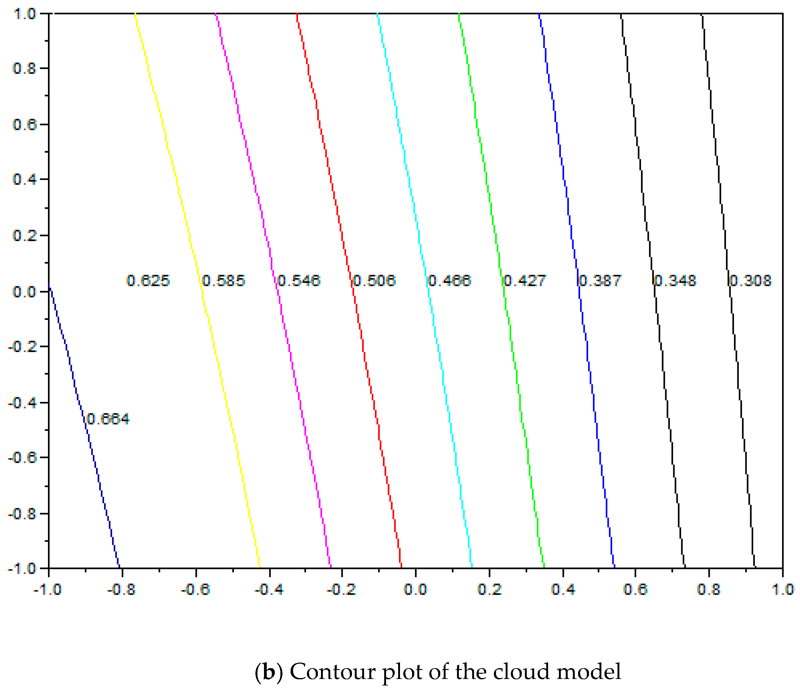
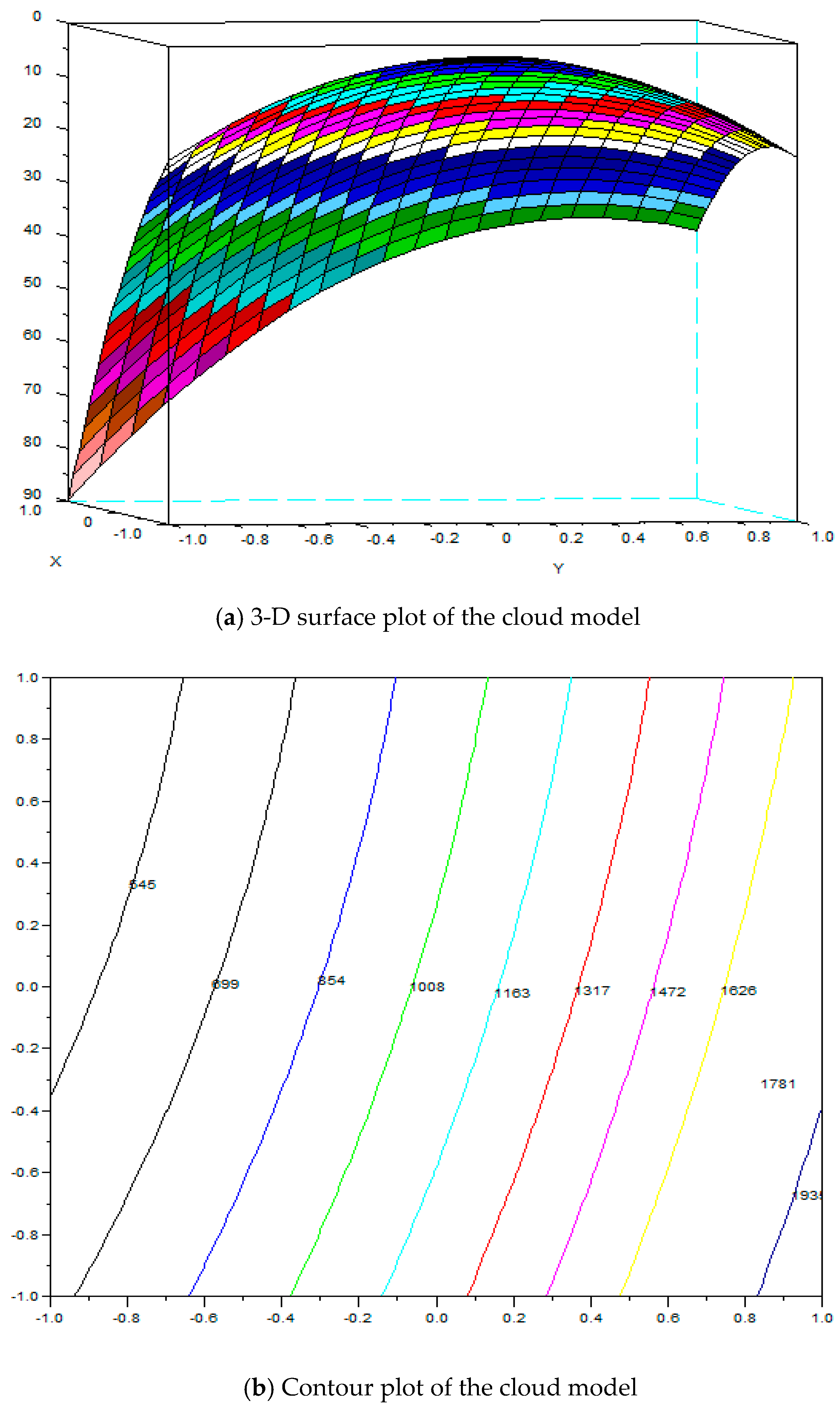
With the above derived system model by response surface method, the optimization process is performed to derive the optimal solution set for this problem. Based on the derived system statistical model, deriving the optimal solution is required. However, the optimal solution may be located anywhere in the range of [−1.0 and +1.0].

The local optimal solution for a non-linear model may not be the optimal one in the global region, therefore, the OPSO process is used to derive the optimal solution in an efficient way. In OPSO method, the local point and global point are searched at the same time and the global optimal solution can be found

By adding random seeds into the formulation, the OPSO method can jump out of the local optimal solution if the global solution is more optimal than the local solution. In the following, the OSPO formulation is performed.

In the response surface method, non-linear problems are approximated as first-order statistical model problems. However, the curvature for this first-order model is large. That means the nonlinearity property is still obvious in this problem. This influences the search process when finding the optimal solution.

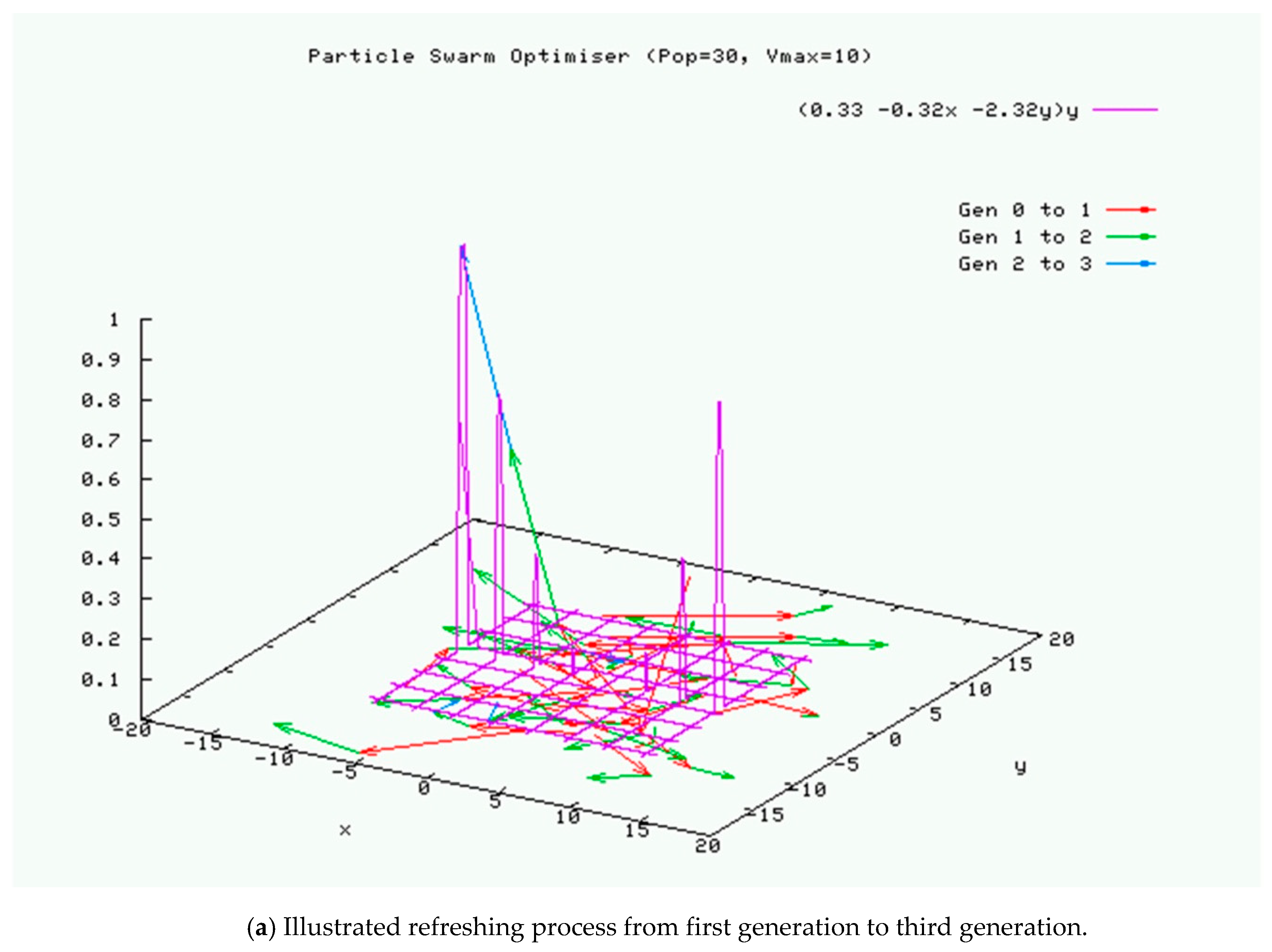
The particle swarm optimization originates from the emulation of the group dynamic behavior of animals. Each particle in a group, is not only affected by its individual behavior, but also by the overall group behavior, so individual and group particles have inter-relations with each other.

There are position and velocity vectors defined for each particle that must be defined first. The searching method combines the contribution of the individual particles with the contributions of the group.

For a particle as a point in a searching space with D-dimension [11,12,13], the i-th particle associated with the problem is defined as:

$$X_{id}=\left(x_{i1},x_{i2},\dots ,x_{iD}\right)$$

(19)

where d = 1, 2, …, D and i = 1, 2, …, PS, PS is the population size.

The respective particle value and group value associated with each particle $X_{id}$ are defined as:

$$P_{pd}=\left(p_{p1},p_{p2},\dots ,p_{pD}\right)$$

(20)

$$P_{gd}=\left(p_{g1},p_{g2},\dots ,p_{gD}\right)$$

(21)

The refreshing speed vector is defined as:

$$V_{id}=\left(v_{i1},v_{i2},\dots ,v_{iD}\right)$$

(22)

The refreshing process is formulated as follows with two random seed terms included:

$$\begin{array}{ll}{V}_{id}^{n+1}=& V_{id}^n+c_1\times rand()\times \left(P_{pd}-X_{id}^n\right)\hfill \\ & +c_2\times rand()\times \left(P_{gd}-X_{id}^n\right)\end{array}$$

(23)

where $X_{id}^{n+1}=X_{id}^n+V_{id}^n$.

When the searching process begins, the initial guess solution is set to begin the process. In the iteration process, the particle is updated by the values coming from both the group contribution and particle contributions. The convergence condition depends on the minimum of the average square error of the particle, and is terminated when the average square error is small.

Both the contribution of the individual particle and the contribution of the group are mixed together into the searching process. In the optimization problem, there might be local minimum problems. The optimal solution might jump into a local trap and be unable to jump out of the trap.

Since there are random seeds in the equation, the local optimal point has the chance to jump out of the local trap area and approach another global one.

An inertia weighting factor is considered in this algorithm to increase the convergence rate. An inertia weighting factor is added in the following expression:

$$W=W_{\max }-\frac{W_{\max }-W_{\min }}{ge{n}_{\max }}\times gen$$

(24)

Therefore, the speed vector modifying process can be rewritten as:

$$\begin{array}{ll}{V}_{id}^{n+1}& =W\times V_{id}^n+c_1\times rand()\times \left(P_{pd}-X_{id}^n\right)\\ & +c_2\times rand()\times \left(P_{gd}-X_{id}^n\right)\end{array}$$

(25)

where the $c_1$ and $c_2$ are both constants, $W_{\max }$ is the initial weighting value, $W_{\min }$ is the final weighting value, gen is the number of current generation, $ge{n}_{\max }$ is the number of final generation.

However, the abovementioned expression corresponds to a linear modification for the two random seed factors. To make the algorithm suitable for a non-linear search problem, there are many non-linear modification methods proposed to refresh the velocity vector. In this case a K factor is defined as follows:

By setting the learning factors $c_1$ and $c_2$ which are larger than 4.0, the modification for the speed vector is expressed as:

$$V_{id}^{n+1}=K\times \left[\begin{array}{l}{V}_{id}^n+c_1\times rand()\times \left(P_{pd}-X_{id}^n\right)\\ +c_2\times rand()\times \left(P_{gd}-X_{id}^n\right)\end{array}\right]$$

(26)

$$K=\frac{2}{\left|2-\left(c_1+c_2-\sqrt{{\left(c_1+c_2\right)}^2-4\times \left(c_1+c_2\right)}\right)\right|}$$

(27)

However, the modified term is quite complicated.

In the following, a modified PSO method called orthogonal PSO (OPSO) is proposed to simplify the formulation and improve the search process effectively.

A simpler orthogonal array in the Taguchi method is used in this algorithm to simplify the searching process.

5.2. Orthogonal Array Algorithm in Cloud Model

To run the Taguchi method, two functions are defined first:

The particle swarms are composed of individual particle swarm $O_{id}$ and group swarm $A_{id}$ respectively: $O_{id}$ and group swarm $A_{id}$ are defined in the following:

$$\begin{array}{ll}{O}_{id}& =X_{id}^n+W{V}_{id}^n\\ & +c_1\times rand()\times \left(P_{pd}-X_{id}^n\right)\end{array}$$

(28)

$$\begin{array}{ll}{A}_{id}& =X_{id}^n+W{V}_{id}^n\\ & +c_2\times rand()\times \left(P_{gd}-X_{id}^n\right)\end{array}$$

(29)

The two functions are specified as two control factors in Taguchi method. Two levels are defined for the control factors, so the orthogonal array has two factors with two levels.

The S/N ratio data for THD and reactive power are used as the experimental runs in orthogonal array. Assume that the optimal solution is expressed as $Q_{id}$. The $Q_{id}$ is adopted to refresh the particle position and velocity vectors as shown in the following expression. The particle refreshing process in OPSO optimization is illustrated in Figure 9.

The developed equation can be simplified as follows:

$$V_{id}^{n+1}=Q_{id}-X_{id}^n$$

(30)

$$X_{id}^{n+1}=Q_{id}$$

(31)

5.3. Optimization Results of Cloud Model

With the above formulation for the optimization problem, the optimal solutions for the reactive power and THD value are found at the same time by using MPCI method. The derived optimal solution can provide the optimal operating conditions for the vehicle-to-grid connected inverter.

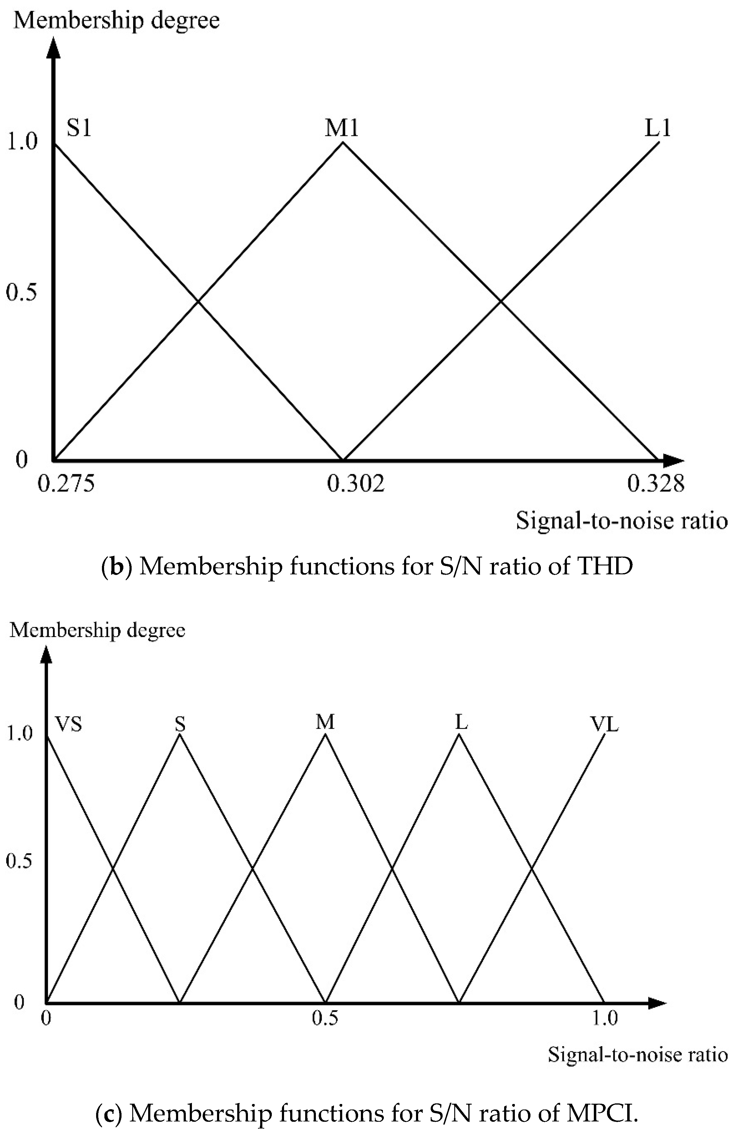
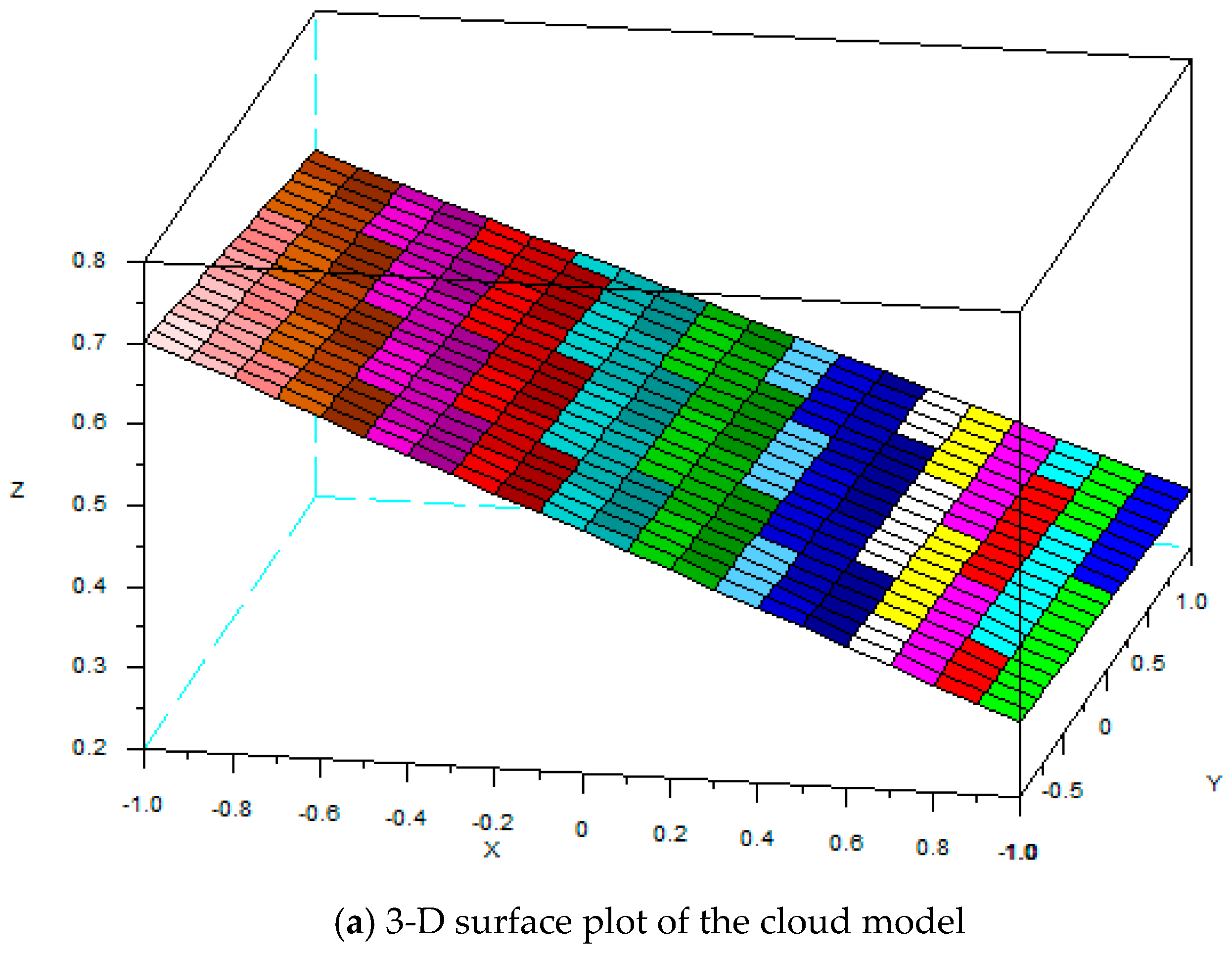
By using the response surface method with OPSO method, the mathematical cloud model for this problem is provided and verified. This is very helpful and useful to assess associated smart vehicle-to-grid applications.

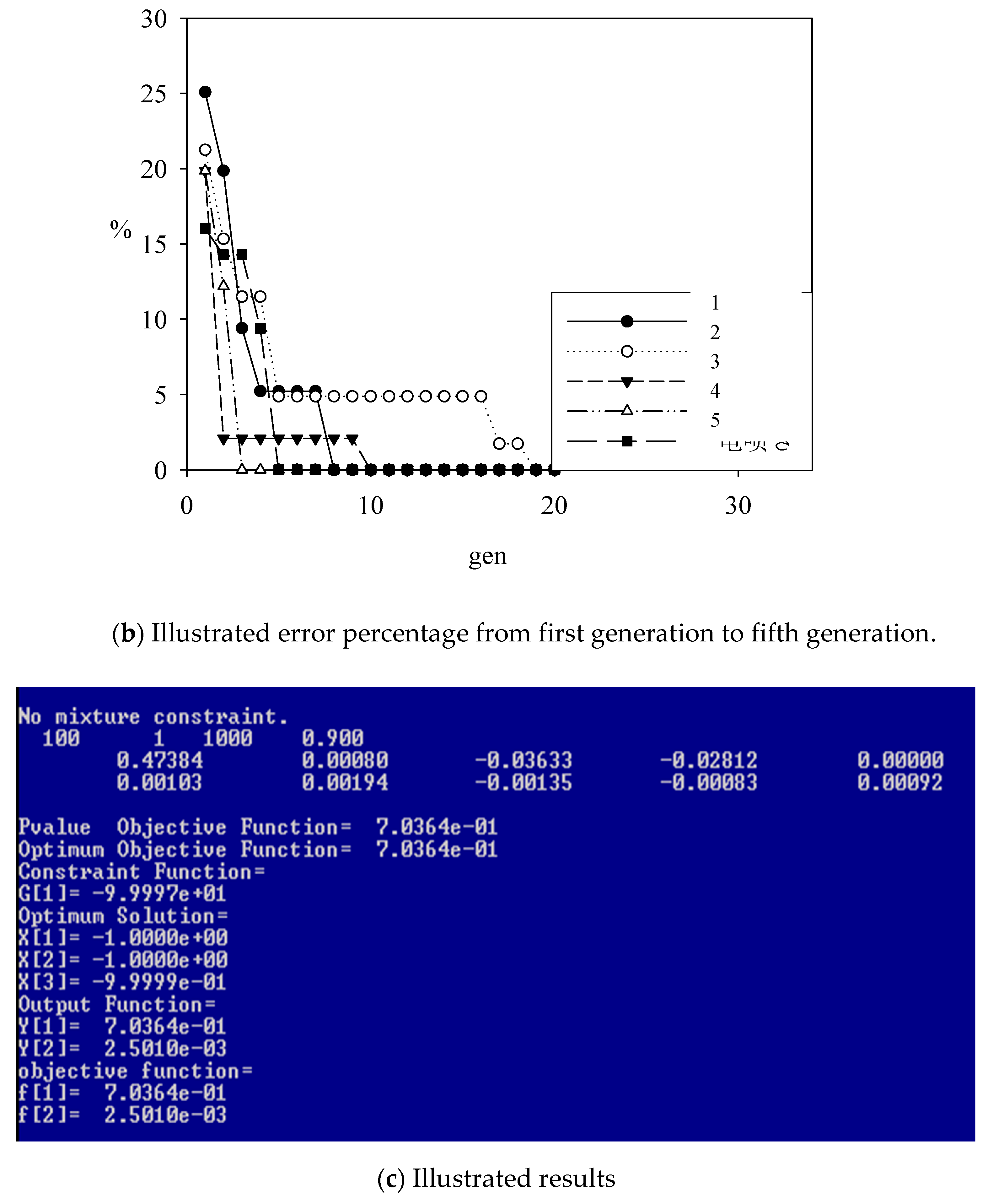
Instead of local solutions and optimal solution can be found and located at the end of the entire searching range. The results show that the proposed mathematical method has the capability of providing a better searching process and through the analysis of response surface method combined with OPSO process, the optimal solution is found.

The optimal solution is located at ($x_1$, $x_2$, $x_3$) = (−1.0, −1.0, −1.0). That is to say, the corresponding optimal parameters for the PID controller are: K_p 12,767, K_i 367 and K_d 1.0 × 10⁻⁵. The optimal solution is observed to correspond to the sixteenth experimental run in the combined array.

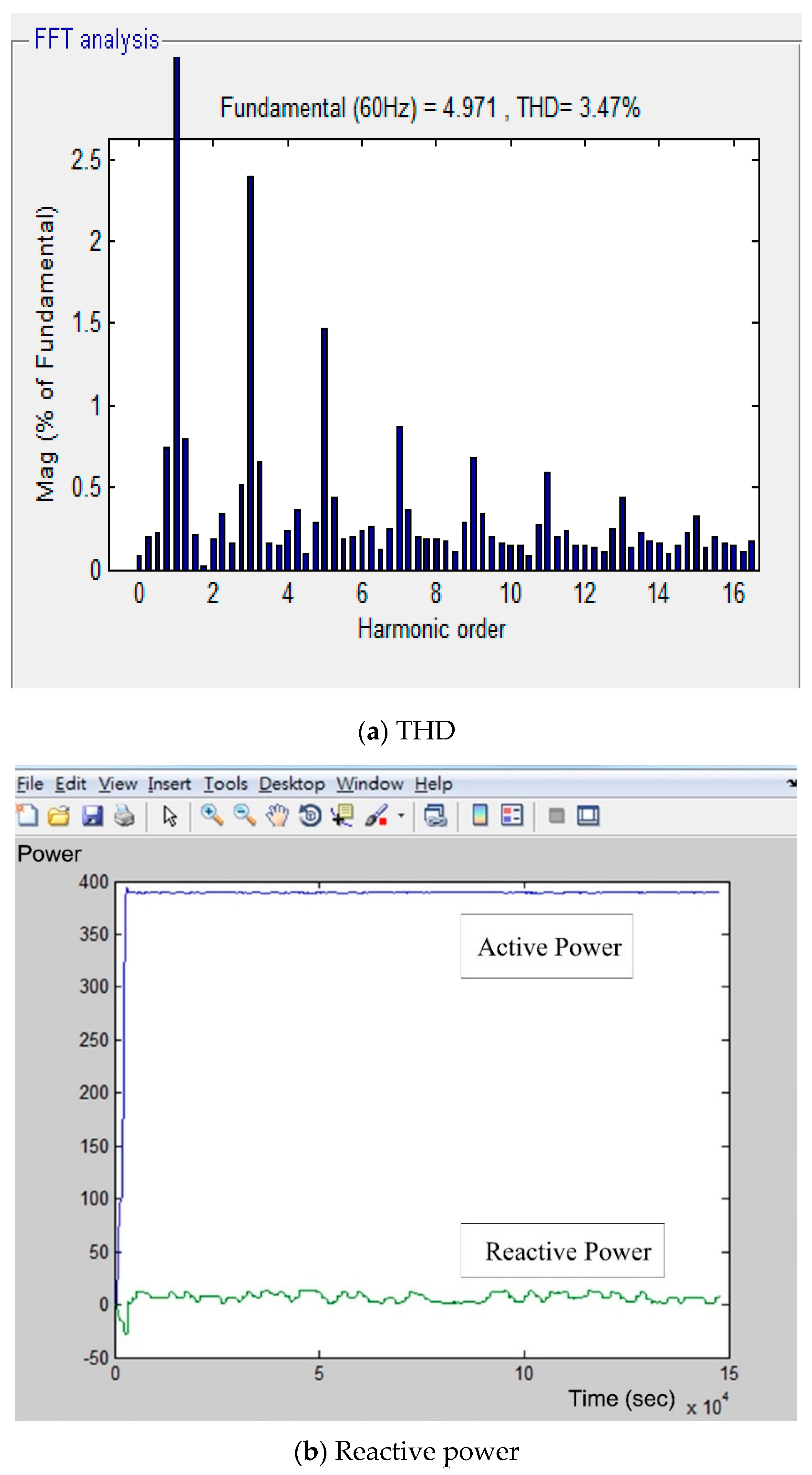
The experimental results show that the reactive power 5.94 Var, 6.94 Var and THD values 3.16%, 3.06% are the minimal values in the combined array.

The results show that there are optimal solutions located at the endpoints of the range [−1.0, 1.0]. The convergence rate is faster than in a conventional searching method. The related confirmation experiments show that the proposed methodology can provide good predictions with the practical experimental runs. It is proved that the proposed optimal parameter solution solved by the OPSO algorithm can minimize the reactive power and THD values for smart vehicle-to-grid problems.

5.4. Testing Results for the Cloud Model

In this paper, a current-controlled single-phase vehicle-to-grid connected inverter is connected to a power system. The electrical voltage is set to be 110 V AC. Both the reactive power and THD is expected to be minimized when the power inverter is working. By using the fuzzy based MPCI and response surface method, the optimal solution can be found.

The above testing cases are compared in

Table 9. Comparison among testing results analyzed by proposed statistical cloud model.

Item	Reactive Power Experiment	THD Experiment	MPCI Experiment
Analysis method	Response surface method	Response surface method	MPCI fuzzy inference response surface method
Objective function	Smaller-the-better	Smaller-the-better	Smaller-the-better
Optimal combination	(1.0, 1.0, −1.0)	(−1.0, −1.0, −0.75)	(−1.0, −1.0, −0.99)
Optimal PID parameters	(52767, 767, 1 × 10−5)	(12767, 367, 1 × 10−5)	(12767, 367, 1 × 10−5)
Data in combined array	5.94 (Var) 6.94 (Var)	3.16 (%) 3.06 (%)	6.89 (Var), 3.16 (%) 6.40 (Var), 3.06 (%)
OPSO solution	6.52 (Var)	3.10 (%)	6.48 (Var), 3.08 (%)

. The first column is an optimization for reactive power only. The second column is an optimization for THD only. The third column is an MPCI optimization problem which considers the reactive power and THD together. In Table 9, the reactive power is reduced to 6.48 Var and THD reduced to 3.08%. The MPCI method is verified to be optimal as compared with the experimental runs in the combined array. In the experimental runs, not only the reactive power is proved to be minimal, but also the THD value is proved to be minimal at the same time.

6. Discussion

Through the above verification, the statistical cloud model suggested that the full-bridge inverter can improve the power factor and minimize the reactive power. The energy losses can be reduced and power transmission quality for the power system is improved. The statistical cloud model includes the multi-objective optimal design by using the fuzzy-based response surface methodology combined with a multiple performance characteristics index. The reactive power and the total harmonic distortion are selected as two major objective functions. Both objectives are achieved to reduce the reactive power and reduce the total harmonic distortion at the same time. The power factor is enhanced and the current waveform is also improved. Testing results show that the proposed optimal cloud model is valid for practical vehicle-to-grid connection application problems.

Due to space limitations, the comparison with other multi-objective methods will be discussed in our future work.

7. Conclusions

This aim of the paper was to provide an optimal design of a statistical cloud model for vehicle-to-grid connected systems. There were two design objectives for the cloud model. The first one was to minimize the reactive power and the second one was to minimize the total harmonic distortion (THD) for the power grid. By using MPCI with a fuzzy-based response surface method, a statistical method was used in the cloud model to analyze the collected data from the cloud database. The testing results analyzed by the proposed cloud model showed that not only was the reactive power minimized but also the THD was minimized under the proposed optimal conditions. It is verified that the cloud model can provide better performance for practical applications of vehicle-to-grid connected systems with IOT.

References

1. Araujo, S.V.; Zacharias, P.; Mallwitz, R. Highly Efficient Single-Phase Transformerless Inverters for Grid-Connected Photovoltaic Systems. IEEE Trans. Ind. Electron. 2010, 57, 3118–3128. [Google Scholar] [CrossRef]
2. Silva, S.M.; Lopes, B.M.; Filho, B.J.C.; Campana, R.P.; Bosventura, W.C. Performance evaluation of PLL algorithms for single-phase grid-connected systems. In Proceedings of the 39th IAS Annual Meeting, Conference Record of the 2004 IEEE Industry Applications Conference, Seattle, WA, USA, 3–7 October 2004; Volume 4, pp. 2259–2263. [Google Scholar]
3. Furuhashi, T.; Okuma, S.; Uchikawa, Y. A Study on the Theory of Instantaneous Reactive Power. IEEE Trans. Ind. Electron. 1990, 37, 86–90. [Google Scholar] [CrossRef]
4. Yafaoui, A.; Wu, B.; Kouro, S. Improved active frequency drift anti-islanding method wit lower total harmonic distortion. In Proceedings of the 36th Annual Conference on IEEE Industrial Electronics Society Conference, Glendale, AZ, USA, 7–10 November 2010; pp. 3216–3221. [Google Scholar]
5. Nonaka, S.; Neba, Y. Single-Phase Composite PWM Voltage Source Converter. In Proceedings of the IEEE Industry Applications Society Annual Meeting, Denver, CO, USA, 2–6 October 1994; Volume 2, pp. 761–768. [Google Scholar]
6. Gaing, Z.L. A Particle Swarm Optimization Approach for Optimum Design of PID Controller in AVR System. IEEE Trans. Energy Convers. 2004, 19, 384–391. [Google Scholar] [CrossRef] [Green Version]
7. Hang, C.C.; Astrom, K.J.; Ho, W.K. Refinements of the Ziegler-Nichols tuning formula. IEE Proc. D 1991, 138, 111–118. [Google Scholar] [CrossRef]
8. Malik, Z.; Rashid, K. Comparison of optimization by response surface methodology withneurofuzzy methods. IEEE Trans. Magn. 2000, 36, 241–257. [Google Scholar] [CrossRef]
9. Zimmermann, H.J. Fuzzy Set Theory and Its Applications; Kluwer Academic Publishers: London, UK, 1985. [Google Scholar]
10. Gaing, Z.L.; Chiang, J.A. Robust design of in-wheel PM motor by fuzzy-based Taguchi method. In Proceedings of the Power and Energy Society General Meeting, Providence, RI, USA, 25–29 July 2010. [Google Scholar]
11. Shi, Y.; Eberhart, R. A modified Particle swarm optimization. In Proceedings of the IEEE International Conference on Evolutionary Computation, Anchorage, AK, USA, 4–9 May 1998; pp. 69–72. [Google Scholar]
12. Eberhart, R.C.; Shi, Y. Comparing inertia weights and constriction factors in particle swarm optimization. In Proceedings of the Congress on Evolutionary Computation, La Jolla, CA, USA, 16–19 July 2000; pp. 84–88. [Google Scholar]
13. Ho, S.Y. Orthogonal Particle Swarm Optimization and Its Application to Task Assignment Problems. IEEE Trans. Syst. Man Cybern. 2008, 38, 288–298. [Google Scholar]
Figure 1. Circuit of single-phase full-bridge inverter for a vehicle-to-grid connected system.
Energies 12 01041 g001
Figure 2. Block diagram of a PID control system for Igrid and Vdc.
Energies 12 01041 g002
Figure 3. Simulink diagram representing a single-phase full-bridge vehicle-to-grid connected system.
Energies 12 01041 g003
Figure 4. Analyzed data and waveforms for the initial design of the single-phase full-bridge vehicle-to-grid connected system.
Energies 12 01041 g004
Figure 5. Flow chart of MPCI method built in cloud model.
Energies 12 01041 g005
Figure 6. Membership functions.
Energies 12 01041 g006aEnergies 12 01041 g006b
Figure 7. The mean response surface of cloud model.
Energies 12 01041 g007aEnergies 12 01041 g007b
Figure 8. The variance response surface of cloud model.
Energies 12 01041 g008
Figure 9. Illustrated OPSO process for the optimization problem.
Energies 12 01041 g009aEnergies 12 01041 g009b