A Transformer Fault Diagnosis Model Based on Chemical Reaction Optimization and Twin Support Vector Machine

Abstract

The condition monitoring and fault diagnosis of power transformers plays a significant role in the safe, stable and reliable operation of the whole power system. Dissolved gas analysis (DGA) methods are widely used for fault diagnosis, however, their accuracy is limited by the selection of DGA features and the performance of fault diagnosis models, for example, the classical support vector machine (SVM), is easily affected by unbalanced training samples. This paper presents a transformer fault diagnosis model based on chemical reaction optimization and a twin support vector machine. Twin support vector machines (TWSVMs) are used as classifiers for solving problems involving unbalanced and insufficient samples. Restricted Boltzmann machines (RBMs) are used for data preprocessing to ensure the effective identification of feature parameters and improve the efficiency and accuracy of fault diagnosis. The chemical reaction optimization (CRO) algorithm is used to optimize TWSVM parameters to select the optimal training parameters. The cross-validation (CV) method is used to ensure the reliability and generalization ability of the diagnostic model. Finally, the validity of the model is verified using real fault samples and random testing.

1. Introduction

With the development of smart grids in power system construction, improving the real-time diagnosis and analysis of the equipment involved represents an urgent technical challenge. The reliability of power transformers, which are critical core equipment in power transmission and distribution systems, dictates the safe and reliable performance of the whole electrical system. Thus, timely discovery of early potential transformer faults is very important and condition monitoring, as well as fault detection, have gradually attracted more and more attention of both the domestic and foreign research communities [1,2,3].

The composition, content, and proportion of dissolved gas in the oil of a power transformer are closely related to the fault type and fault degree of the transformer, which effectively reflect the operation state of a transformer. Dissolved gas analysis (DGA) is the most convenient and effective method available for early potential fault diagnosis of oil-immersed transformers because it is an accurate and reliable method to find potential faults inside a transformer of this type. The improved/new three-ratio (IEC three-ratio) and Dornerburg method are effective methods for oil-immersed transformer fault diagnosis, being easily implemented and widely used. These traditional DGA methods mainly use operational experience and expert knowledge to establish the diagnosis rules of "code-fault type" based on the ratio (or content) of dissolved gas and fault types, but these methods suffer some drawbacks in their engineering applications, such as their code boundaries being excessively absolute and faults not being completely covered by the defined codes [4,5].

With the development of artificial intelligence (AI), machine learning (ML), data mining (DM), and other theories and technologies, the data-driven intelligent model has been applied to transformer fault diagnosis. The use of the artificial neural network (ANN) [6,7], expert system, Bayes network, support vector machine (SVM) [8,9], random forest (RF), and other theories and methods have provided new ideas for transformer fault diagnosis. However, all AI diagnostic methods have some limitations. For example, ANN needs to be prevented from overfitting and is susceptible to local extrema, the completeness of an expert system knowledge base cannot be guaranteed, a Bayes network needs a large number of sample data, and matter-element theory has strict requirements on sample consistency and sample size.

The input parameters of AI fault diagnosis methods are mainly derived from the gas ratio or content of DGA methods recommended by the International Electrotechnical Commission (IEC) and Institute of Electrical and Electronics Engineers (IEEE), but some important features are neglected by the input parameters of these methods and the feature sets need to be improved. Normal and fault states of transformers cannot be distinguished by these methods, which limits their application in online monitoring and fault diagnosis. At the same time, in the actual work of operating and maintaining transformers, fault samples and data are difficult to collect and the types of fault are diverse, so it is difficult to assemble massive and complete fault samples. Meanwhile, the collected fault samples are often unbalanced, therefore, the application in practical work of AI diagnostic methods has been limited by these conditions.

SVM has a high generalization ability, no neural network overfitting, slow convergence, and can be easily affected by local extrema. Therefore, SVM is suitable for nonlinear, local minimum point, and small sample pattern recognition, and other practical problems. However, SVM is easily affected by unbalanced samples [10,11,12]. To overcome this disadvantage, researchers have introduced many modification methods, and twin support vector machine (TWSVM) is the most commonly applied among them. TWSVM is used as the classifier to address the potential unbalanced sample issue associated with SVMs and to increase the SVM training speed. TWSVM can apply different penalty factors to the two categories of samples if the samples are not balanced.

In this study, we propose a transformer fault diagnosis model based on chemical reaction optimization and a TWSVM based on the status of the power industry and the characteristics of transformer fault diagnosis. A variety of DGA fault diagnosis feature parameters are fused as the input parameters of the model to solve the problems of too absolute coding boundary and incomplete coding coverage of faults. TWSVMs are used as classifiers for solving the problems of unbalanced and insufficient samples. The restricted Boltzmann machine (RBM) is used for data preprocessing to ensure the effective identification of feature parameters and improve the efficiency and accuracy of fault diagnosis. A chemical reaction optimization (CRO) algorithm is used to optimize TWSVM parameters (penalty factors and kernel parameter) to select the optimal training parameters. We used cross-validation (CV) to ensure the reliability and generalization ability of the diagnostic model. Finally, the validity of the model was verified using real fault samples and random testing.

The remainder of this paper is organized as follows: Section 2 outlines related work on transformer fault diagnosis techniques. Section 3 covers fundaments of CRO-TWSVM model. The transformer fault diagnosis model based on CRO-TWSVM is presented in Section 4. Examples of the transformer fault diagnosis model are given in Section 5. Finally, conclusions are drawn and potential future work is discussed is Section 6.

2. Related Work

With the rapid development of computer technology and artificial intelligence (AI) theory, machine learning-based techniques and data-driven modeling methods, including artificial neural network (ANN) [13,14,15,16,17], fuzzy theory [18,19], expert system (EPS) [20], rough sets theory (RST) [21], and other intelligent diagnosis methods [22,23,24,25,26,27,28,29,30,31] such as random forest (RF), gradient boosting decision tree (GBDT), deep belief network (DBN), support vector machine (SVM) and evidential reasoning approach, have been introduced to the research field of transformer fault diagnosis based on the DGA approach. These intelligent methods make up for the deficiencies of the mentioned traditional DGA methods, and directly or indirectly improve the accuracy of transformer fault diagnosis, and provide a new train of thought for high-precision transformer fault diagnosis.

Guardado et al [15] demonstrate that IEC based BP neural network can acquire a higher accuracy rate than other DGA methods in fault detection. Yang et al [16] proposed a multi-level BP neural network fault diagnosis model for transformer. Wang et al. [17] present a novel method for power transformer fault diagnosis based on probability neural network (PNN) and dissolved gas analysis, they used a new hybrid evolutionary algorithm combined with a particle swarm optimization (PSO) algorithm and back propagation (BP) algorithm to optimize the parameters of PNN. Illias et al. [7] proposed an improved hybrid modified evolutionary particle swarm optimizer (PSO) time varying acceleration coefficient-ANN for power transformer fault diagnosis. Rigatos et al [23] proposed neural modeling and local statistical approach to fault diagnosis for the detection of incipient faults in power transformers, which can detect transformer failures at their early stages and consequently can avoid critical conditions for the power grid, furthermore, the random forest technique-based fault discrimination scheme [25] for fault diagnosis of power transformers, as well as the multi-layer perceptron (MLP) neural network-based decision [30], and have been proposed consecutively. The authors of [18] proposed a deep belief network (DBN) approach to predict transformer concentrations. They achieved good prediction accuracy, but their method ignores the relationship between the individual gas components.

Through the optimization of different ANN approaches, the above methods to some extent solve the problems that the neural network is easy to overfit, has slow convergence speed, easily gets into local minima, and achieve good results, but the premise is the availability of a large number of samples as support. In the same way, other ML methods, such as RF, DBN also need a large number of samples. However, in the actual work of transformer operation and maintenance, fault samples and data are difficult to collect and the types of fault are diverse, so it is difficult to form massive and complete fault samples.

SVM, proposed by Vapnik, is a machine learning method developed from statistical theory. SVM adopts the principle of structural risk minimization and is suitable for training and classification of small samples. The authors of [32,33,34,35,36,37,38] proposed support vector machine (SVM)-based intelligent fault classification approaches for power transformer DGA. Zhang et al. [37] developed a useful approach combing the wavelet technique with a least squares support vector machine (LS-SVM) based on particle swarm optimization (PSO) with mutation for forecasting of dissolved in the power transformer. There are also many research efforts focusing on fault detection for another equipment and systems. Li et al. [38] presented an intelligent method for the fault diagnosis of power transformers based on selected gas ratios and SVM. They used a genetic algorithm (GA) to obtain the optimal dissolved gas ratios (ODGR) which is used for the DGA ratio selection and SVM parameters optimization. Liu et al. [35] presented a fault classification approach for power transformer using DGA and SVM algorithm. They used training data to build a multi-layer SVM classifier. Such a classifier has a good performance in identifying the transformer fault types.

The mentioned intelligent approaches have improved the conventional DGA-based transformer fault diagnosis methods, and directly or indirectly improved the accuracy of fault diagnosis for the power transformers. However, these studies tend to focus on model selection and optimization, and the problem of unbalanced samples in the case of small samples is not well solved. Meanwhile, there are deficiencies in the training methods and data preprocessing methods. These problems limit the practical application of AI algorithm or model in transformer fault diagnosis. Therefore, in this paper, the CRO-TWSVM model is proposed to solve these problems.

3. Fundaments of CRO-TWSVM Model

3.1. Restricted Boltzmann Machine

In 1986, on the basis of the Boltzmann machine, Smolensky proposed a stochastic neural network model named Restricted Boltzmann Machines (RBM) [39]. An RBM network is composed of a hidden layer and a visible layer. The visible layer is composed of visible units, which can be used to receive the input of transformer characteristic parameters, and the hidden layer is composed of hidden units, which can be used to extract the deep feature vectors. The units on the same layer are not connected, and the units on different layers are connected to each other.

The state of each RBM unit is random, and 1 or 0 is used to indicate whether the unit is active or not, and the state is determined by energy probability statistics method.

Suppose RBM has n visible units and m hidden units, and the bias weights of visible layer are defined as a = {a₁,a₂,…,a_n}, the bias weight of hidden layer are defined as b = {b₁,b₂,…,b_m}, the weights of connection between hidden units and visible units are defined as ω = {w₁₁,w₁₂,…,w_nm}, then the RBM’s parameters can be defined as θ = {ω,a,b}. Given these, the energy of a configuration of RBM is defined as:

$$E(v,h|\theta )=-{\displaystyle \sum _{i=1}^n{a}_i{v}_i}-{\displaystyle \sum _{\mathrm{j}=1}^m{b}_i{h}_i-}{\displaystyle \sum _{i=1}^n{\displaystyle \sum _{\mathrm{j}=1}^m{\omega }_{ij}{v}_i^{}{h}_j}}$$

(1)

where: ν_i is the state of the i-th visible unit, a_i is the bias weight of i-th visible unit, ν = {ν₁,ν₂,…,ν_n} is the state of the visible layer, h_j is the state of j-th hidden unit, b_iis the bias weight of j-th hidden unit, h = {h₁,h₂,…,h_m} is the state of hidden layer, w_ij is the weight of connection between the i-th visible unit and the j-th hidden unit.

The activated probability of i-th visible unit and the j-th hidden unit can be obtained by the following equation:

$$\begin{array}{l}p(v_i=1|h)=\sigma (a_i+{\displaystyle \sum _{\mathrm{j}=1}^m{h}_j{w}_{ij}})\\ p(h_j=1|v)=\sigma (b_i+{\displaystyle \sum _{i=1}^n{v}_j{w}_{ij}})\end{array}$$

(2)

where:

$$\sigma (x)=\frac{1}{1+e^{-x}}$$

(3)

and the probability that RBM in the state of (ν,h) can be obtained by the following equation:

$$p(v,h|\theta )=\frac{e^{-E(v,h|\theta )}}{{\displaystyle \sum _{v,h}{e}^{{}^{-E(v,h)}}}}$$

(4)

Suppose the total number of training samples is Q, the i-th sample can be defined as ${\nu }^q=\left\{{\nu }_1^q,{\nu }_2^q,\dots ,{\nu }_{\mathrm{n}}^q\right\}$. The likelihood function of Equation (5) can be maximized through training, and the parameters of RBM θ = {ω,a,b} can be obtained.

$$L(\theta )={\displaystyle \prod _{q=1}^{Q}P(v^q)}$$

(5)

By using the Contrastive Divergence (CD) algorithm proposed by Hindon, the parameters of RBM can be described as Equation (6):

$$\begin{array}{l}{w}_{ij}(t+1)=w_{ij}(t)+\epsilon ({(v_i{h}_j)}_{data}-{(v_i{h}_j)}_{recon})\\ a_i(t+1)=a_i(t)+\epsilon ({(v_i)}_{data}^{}-{(v_i)}_{recon})\\ b_j(t+1)=b_j(t)+\epsilon ({(h_j)}_{data}^{}-{(h_j)}_{recon})\end{array}$$

(6)

where, [□]_data is the expected value of the given data, [□]_recon is the mathematical expectation of the reconstructed model, ε is the learning rate for the parameters of the RBM.

Studies have shown that RBM can improve the recognition accuracy and training speed of classification model through data preprocessing and the RBM preprocessing method proposed for Finger Motion Estimation by Mousas [40] works well.

Based on the aforementioned process, RBM is used to preprocess the transformer diagnosis features. The DGA parameters of transformer are set as the input elements of visible layer, the hidden layer stands for a non-linear transformed feature space, and the hidden layer’s units, as a hyper-parameter, define the dimensionality of the new feature space. Finally, the output vector preprocessed by RBM is used as the input of the TWSVM in the following section.

3.2. Twin Support Vector Machine

SVM, proposed by Vapnik, is a machine learning method developed from statistical theory. SVM adopts the principle of structural risk minimization to classify data by constructing the optimal hyperplane. It can effectively solve small sample, non-linear, and high dimension classification problems, and has the advantages of fast calculation speed and strong generalization ability, so it has been widely examined and applied [9,33,34].

Given a set of data $\mathrm{T}={\left\{x_i,y_i\right\}}_{i=1}^m$, where X_i ∈ Rⁿ denotes the input vectors, y_i ∈ {+1,–1} is two classes of output, and m is the sample number. The sample set can be constructed into the following classification planes:

$$f(x)=sign(\omega x+b)$$

(7)

where ω denotes the weight vector and b denotes the bias term. ω and b are used to define the position of the separating hyperplane.

The problem of seeking the optimal classification hyperplane can be transformed into a constrained quadratic optimization problem by comprehensively considering structural risk minimization criteria, regularization terms, and fitting errors. The optimal hyperplane separating the data can be obtained by the following equation:

$$\min J(\omega ,\xi )=\frac{1}{2}\left|\right|\omega {\left|\right|}^2+\mathrm{C}{\displaystyle \sum _{i=1}^m{\xi }_i}$$

(8)

where C is the penalty factor and ${\xi }_i$ is the slack factor. Positive slack variables ${\xi }_i$ are introduced to measure the distance between the margin and the vectors x_i that lie on the wrong side of the margin. The Lagrange coefficient method is used. By introducing the Lagrangian multiplier α_i, the optimal hyperplane is:

$$f(x)=sign({\displaystyle \sum _{i,j=1}^m{\alpha }_i{y}_i}(x_i,x_j)+b)$$

(9)

SVM can also be used in nonlinear classification by using the kernel function. Using the nonlinear mapping function $\phi (·)$, the original data x are mapped into a high-dimensional feature space, where the linear classification is possible. Then, the nonlinear decision function is:

$$f(x)=sign({\displaystyle \sum _{i,j=1}^m{\alpha }_i{y}_i}K(x_i,x_j)+b)$$

(10)

where $K(x_i,x_j)$ is the kernel function, $K(x_i,x_j)=\phi (x_i)\phi (x_{\mathrm{j}})$.

TWSVMs generate two unparalleled classification hyperplanes by converting one quadratic programming problem (QPP) of a classical SVM into two QPPs, but of a smaller size.

The basic idea of TWSVM is to construct two unparalleled hyperplanes in an n-dimension space:

$$\begin{array}{l}K{(\mathrm{x}}^{\prime }{,\mathrm{c}}^{\prime }){\omega }^{\left(1\right)}+b^{(1)}=0\\ K{(\mathrm{x}}^{\prime }{,\mathrm{c}}^{\prime }){\omega }^{\left(2\right)}+b^{(2)}=0\end{array}$$

(11)

Each hyperplane occurs such that the samples are as close as possible to the category to which they belong and as far as possible from the categories to which other samples belong. The TWSVM solves the following two quadratic optimization problems:

$$\begin{array}{l}\underset{w^{(1)}.b^{(1)}}{\min }\frac{1}{2}{\Vert K(A,C^{\prime }){\omega }^{\left(1\right)}+e_1{b}^{(1)}\Vert }^2+c_1^{}{e}^{\prime }{}_{2}q\\ s.t.-(K(B,C^{\prime }){\omega }^{\left(1\right)}+e2b^{(1)})+q\ge e_2\\ \underset{w^{(2)}.b^{(2)}}{\min }\frac{1}{2}{\Vert K(A,C^{\prime }){\omega }^{\left(1\right)}+e_1{b}^{(1)}\Vert }^2+c_1^{}{e}^{\prime }{}_{2}q\\ s.t.-(K(B,C^{\prime }){\omega }^{\left(1\right)}+e2b^{(1)})+q\ge e_1\end{array}$$

(12)

where K represents the kernel function; A and B represent $m_1$ positive category samples and $m_2$ negative category samples, respectively; $e_1$ and $e_2$ are unit vectors with the same number of dimensions with kernel function $K(A,C)$ and $K(B,C)$, respectively; $c_1^{}$ and $c_2^{}$ are penalty factors; $\omega$ and $b$ are the normal vector and the offset of the optimum hyperplane, respectively; and q is the slack factor.

Each of the hyperplanes corresponds to a sample category. The category of a sample depends on the distance between the sample and the hyperplane, with the decision function being:

$$K(x^T,C^T)w_r{+b}_r=\underset{l=1,2}{\min }\left|K(x^T,C^T)w_l+b_l\right|$$

(13)

For a binary classification problem, the space complexity of a standard SVM is O(m³), where m is the number of samples. Supposing each category contains m/2 samples, the space complexity would be $\mathrm{O}(2\times {(\frac{m}{2})}^3)$ if two QPPs are considered. Thus, TWSVM has a space complexity 1/4 that of SVM. With the two penalty factors c₁ and c₂ built into TWSVM, it is also possible to apply different penalty factors to the two categories of samples to solve the classification accuracy concern typical of a classical SVM arising from unbalanced samples [10,11]. TWSVM is employed as the classifier to address the potential unbalanced sample trouble associated with SVMs and to increase the SVM training speed.

3.3. Multi-Category Classification Algorithm

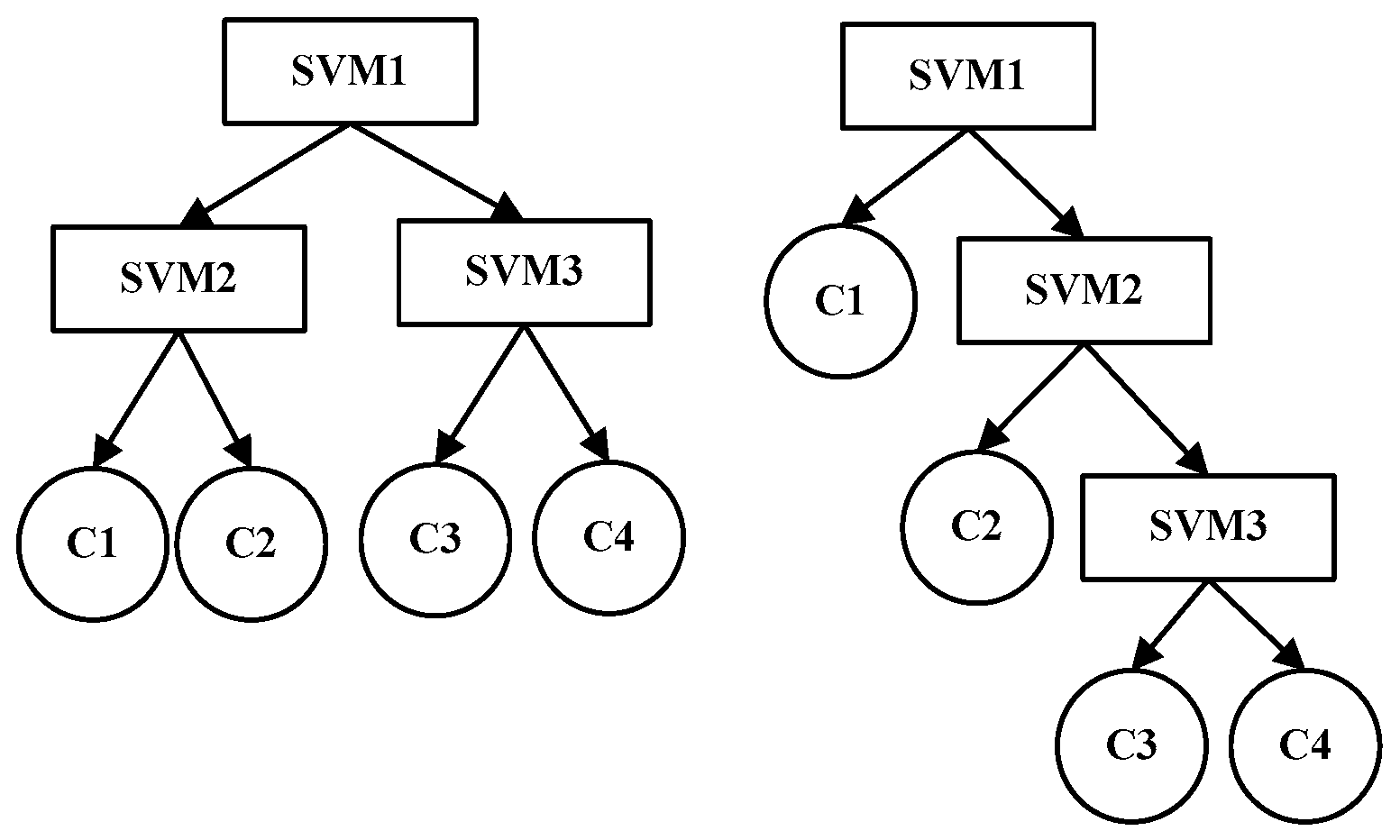
A standard SVM is a binary classifier. For multi-category classification problems, a combinational multi- category classification SVM is generally used; the problem is decomposed and reconstructed into multiple binary classification problems, which are then solved one-by-one.

Among commonly used multi-category classification algorithms are one vs. one, one vs. many, decision directed acyclic graph (DAG), and binary tree algorithms. A binary tree algorithm has the following benefits: (1) ability to fuse with a classification model of interest; (2) for k-category classification problems, only k-1 binary classifiers are needed, which is the least among the aforementioned algorithms and thus the least computation-intensive; (3) the samples required decrease from layer to layer, resulting in a quicker and more efficient training for a given number of layers; and (4) there are no inseparable zones [33,34,35]. We selected the binary tree algorithm to construct a hierarchical TWSVM decision model.

As shown in Figure 1, a classification problem is either a complete or a partial binary tree classification problem. The left figure illustrates a complete binary tree SVM (BT-SVM), wherein each decision node divides its categories into two sub-categories of equal size; the right figure shows a PBT-SVM, wherein each decision node singles out a category from the rest.

3.4. Chemical Reaction Optimization Algorithm

Chemical reaction optimization (CRO) is a metaheuristic algorithm having just emerged in recent years. It is a swarm intelligent algorithm implemented by simulating the molecular movement and energy conversion process in a chemical reaction. It is known that the molecular state in a container is unstable at the beginning of reaction due to excessive energy in the molecules, and the molecules are transferred to the lowest possible energy state through processes facilitated by intermolecular collisions and post-collision chemical reaction in order to achieve a stable state. The ultimate outcome of a chemical reaction is the reaction products, which are formed in a process characterized by a diminishing reaction potential energy. It means that the CRO is an optimization process in which the potential energy of the search system is minimized [41,42,43,44,45,46].

Over the past recent years, metaheuristic algorithms have found extensive applications in various domains and have evolved into GA, particle swarm optimization, ant colony algorithms, etc. Relative to other swarm intelligent algorithms, CRO is good at finding a global solution and producing a shorter optimization time, and thereby, it provides a new idea for solving an optimization problem.

The basic operation units involved in CRO algorithm are composed of molecules (ω) and container walls (buffer), where the molecules possess both potential energy (PE) and kinetic energy (KE) whereas the container walls create the environment in which the reaction occurs. The molecular PE is the ultimate criterion for evaluating a chemical reaction and thus becomes the objective function of the question of interest while the KE is a quantized value for determining whether the system is able to initiate a molecular reaction. In a chemical reaction, there are four basic reaction operators: monomolecular collision, monomolecular decomposition, intermolecular collision, and molecule synthesis. The following paragraphs provide a brief description of the four basic reaction operators [47].

(1) Monomolecular collision

Monomolecular collision is a process in which the KE and PE of a molecule change due to the collision between the wall and the molecule. The energy change occurring in a molecular collision reaction process may be described by Equation (14):

$$K{E}_{{\omega }^{\prime }}=(P{E}_{\omega }-P{E}_{{\omega }^{\prime }}+K{E}_{\omega })\times \delta$$

(14)

where, ω is the original molecule, ω’ is the new molecule after structural change, $\delta \in [KELossRate,1]$ is a random number, $KELossRate$ is the upper limit (in percentage) of monomolecular collision loss rate, being a constant, and $P{E}_{\omega }=f\left(\omega \right)$ is molecular potential energy, with $f(·)$ being the objective function of the problem considered. Monomolecular collision enables local searching in the problem space.

(2) Monomolecular decomposition

Monomolecular decomposition is a reaction occurring when a molecule with higher KE collides with the wall and during which the molecule decomposes or breaks up into two new molecules. The energy difference E_dec existing before and after collision is transmitted to the two new molecules in a random manner; such energy change in this reaction process may be expressed by Equation (15):

$$\begin{array}{l}{E}_{\mathrm{dec}}=(P{E}_{\omega }+K{E}_{\omega }+{\delta }_1\times {\delta }_2\times \mathrm{buffer})\\ -(P{E}_{{\omega }_1{}^{\prime }}+P{E}_{{\omega }_2{}^{\prime }}),\\ K{E}_{{\omega }_1{}^{\prime }}=E_{\mathrm{dec}}\times {\delta }_3,\\ K{E}_{{\omega }_2{}^{\prime }}=E_{\mathrm{dec}}\times (1-{\delta }_3)\end{array}$$

(15)

where ${\delta }_1$,${\delta }_2$ are of uniform distribution in [0, 1] and ${\delta }_3$ is a random value in [0, 1]. Compared to monomolecular collision, monomolecular decomposition is capable of local search in a larger scope.

(3) Intermolecular collision

Intermolecular collision refers to a process in which two new molecules are produced after collision, and energy exchange, between two molecules, while involving no synthesis of molecules. A new molecule may be taken from the original molecular domain and, due to the absence of a collision with the wall, no energy is lost, hence the total energy does not change after the reaction. The two new molecules have a total KE of E_inter, which is distributed among them randomly; the energy change in this reaction process may be described using Equation (16):

$$\begin{array}{l}{E}_{\mathrm{inter}}=(P{E}_{{\omega }_1}+P{E}_{{\omega }_2}+K{E}_{{\omega }_1}+K{E}_{{\omega }_2})\\ -(P{E}_{{\omega }_1{}^{\prime }}+P{E}_{{\omega }_2{}^{\prime }}),\\ K{E}_{{\omega }_1{}^{\prime }}=E_{\mathrm{inter}}\times {\delta }_4,\\ K{E}_{{\omega }_2{}^{\prime }}=E_{\mathrm{inter}}\times (1-{\delta }_4)\end{array}$$

(16)

where ${\delta }_4$ is a random value in the range of [0, 1].

(4) Molecule synthesis

Molecule synthesis refers to the phenomenon where a new molecule is produced after the collision of two molecules. As with intermolecular collision, it is a process involving no wall collision and so the energy remains constant before and after collision. The energy change in this reaction may be described by Equation (17):

$$K{E}_{{\omega }^{\prime }}=(P{E}_{{\omega }_1}+P{E}_{{\omega }_2}+K{E}_{{\omega }_1}+K{E}_{{\omega }_2})-(P{E}_{{\omega }^{\prime }})$$

(17)

Molecule synthesis reactions greatly augment the molecule diversity and the synthesized new molecules differ appreciably from their predecessors and typically possess higher molecular PE. Molecule synthesis reaction improves molecular search power in new regions, hence enhancing CRO’s global search performance.

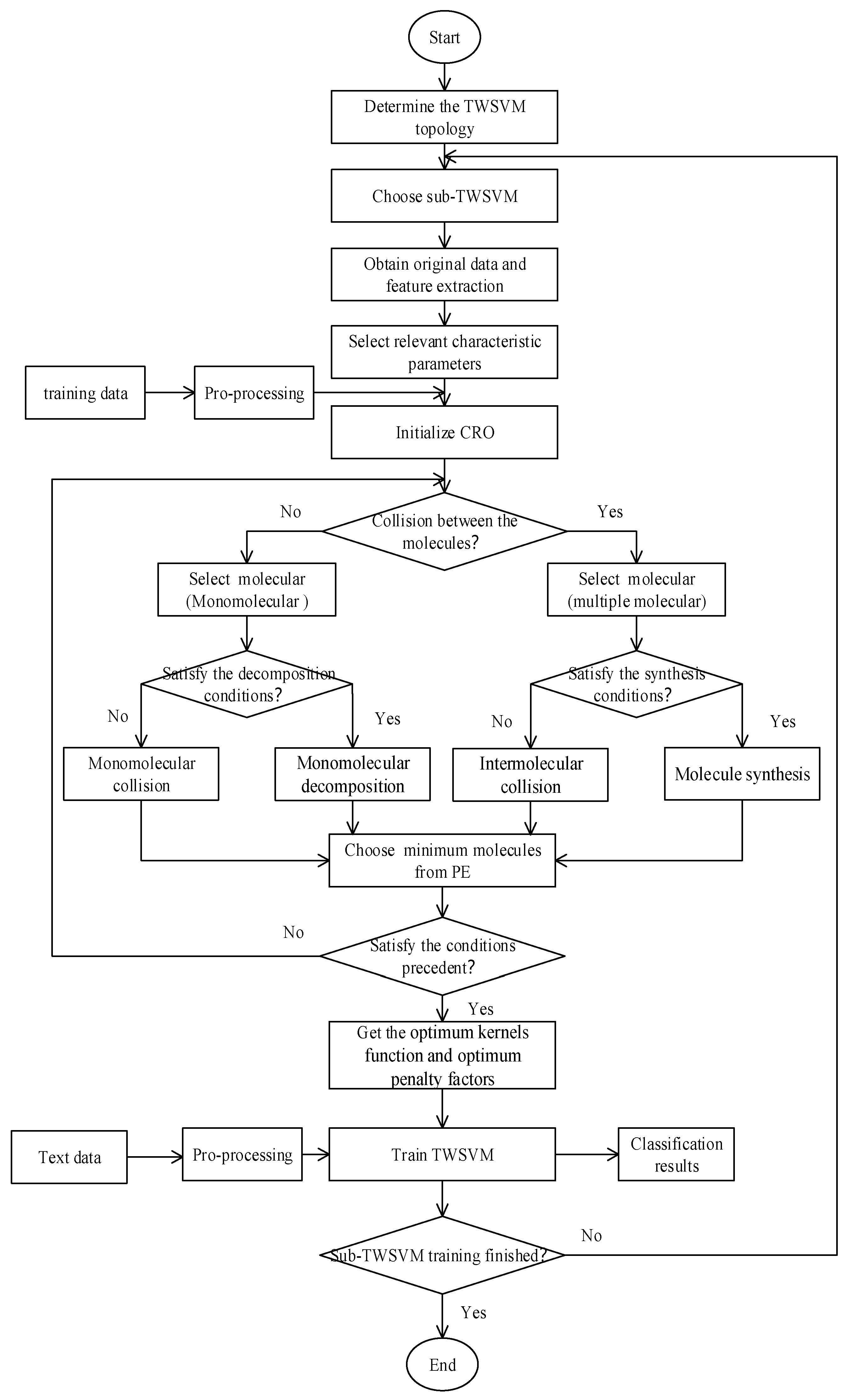
3.5. CRO-TWSVM Modeling Method

CRO-TWSVM model uses the CRO algorithm to optimize TWSVM’s penalty factors and kernel widths, arriving at the optimum penalty factors and kernel widths through iterative optimization involving the four reaction operators. A globally optimum SVM fault diagnosis model is then generated following training using the training sample. The actual procedures are illustrated below, where Figure 2 is depicts the flow chart of CRO-TWSVM modeling.

3.5.1. Pre-Processing

The original DGA samples were normalized to avoid the difference in the order of magnitude of the values of the input parameters. The contents of dissolved gas were converted into the relative content within the range of [0,1], which is conducive to reducing the mutual exclusion between gases. The normalization treatment is described in Equation (18):

$$x_{ij}^{\prime }=x_{ij}^{}/{\displaystyle \sum _{j=1}^k{x}_{ij}^{},i=1,\dots ,n}$$

(18)

The RBM method was used to preprocess the input vector of TWSVM and the feature space was transformed into an appropriate representation, which is conducive to the machine learning of the TWSVM classifier. After being processed by RBM, the transformer fault sample set can be described as a feature set {(y₁,l₁),(y₂,l₂),…,(y_n,l_y)}, where y_i ∈ R_d is the characteristic output of the i-th transformer fault sample, d is the characteristic dimension, n is the number of training samples, $l_i\in \left\{\pm 1\right\}$ represents the output target (I = 1, 2..., N).

3.5.2. Set the Objective Function

We set the objective function along with the initial values of parameters c₁, c₂ and q with regard to the actual problem. Cross-validation is used to eliminate the training bias caused by randomness and evaluate the performance of the training model and improve the stability and generalization ability of the model.

The average classification accuracy of k-fold cross-validation is taken as the object function f to minimize the error of the trained TWSVM model. Considering the sample size and training efficiency, a five-fold cross-validation method was adopted:

$$\begin{array}{l}f=\frac{1}{k}{\displaystyle \sum _{i=1}^k(\frac{l_T^i}{l^i}\times 100\%)}\\ \end{array}$$

(19)

where lⁱ is the number of samples in the i-th verification set, and $l_T^i$ is the number of samples correctly classified in the verification set.

3.5.3. Initialize the CRO Algorithm

In this step, the following quantities are determined: the initial number of molecules in the container (PopSize), the upper limit (in percentage) of KE loss due to wall-collision reaction ($\mathrm{KE}LossRate$), the factor determining the type of molecular reaction (MoleColl), the factor determining the type of monomolecular reaction (α), the factor determining the type of multimolecular reaction (β), and the maximum number of iterations (Iteration).

3.5.4. Compute the Initial PE and KE of Molecules

The initial PE of each molecule is estimated using Equation (11) and the initial value of molecular KE is taken as the initial KE.

3.5.5. Iteration and Optimization

In this step, iterative optimization of the molecules in the container is performed using the four basic reaction operators, with each iteration involving only one basic operator. An iteration operation is composed of three judgment processes, during which the reaction type, the monomolecular reaction type, and the intermolecular reaction type are determined. A judgment is determined based on the random number; if t > MoleColl, then no intermolecular reaction exists and the reaction is instead monomolecular, or vice versa. In the case of a monomolecular reaction, if NumHit–MinHit > α, then proceed with monomolecular decomposition reaction; otherwise, the reaction is monomolecular, where NumHit is the number of collisions, and MinHit is the minimum number of collisions. In the case of a multimolecular reaction, if KE < β, then proceed with molecule synthesis reaction, otherwise proceed with intermolecular collision reaction.

3.5.6. End the Algorithm

If the molecular behavior is such that the algorithm may be ended, then end the optimization process.

3.5.7. Train the Diagnosis Model

The molecule with the minimum PE corresponds to the global optimum solution, which is associated with the kernel width and penalty factor of the optimized TWSVM. The width and factor values are then assigned to TWSVM, which is trained using the training sample to produce the transformer fault diagnosis model.

3.5.8. Testing

Finally, the model is tested for accuracy.

4. A Transformer Fault Diagnosis Model Based on CRO-TWSVM

4.1. Choice of Parameters

The fault diagnosis model parameters are derived from the input characteristic values of the fault diagnosis methods recommended by IEC and IEEE, which are mainly divided into two categories: the input parameters of the IEC method, Roger method (RRM), and Doernenburg method (DRM) are gas ratios; and the input parameters of the key gas method (KGM), David triangle method (DTM) are gas contents.

The feature parameters in the above methods are extracted and repeated features are removed. C₂H₂/C₂H₄ and CH₄/H₂ ratios provide a good discriminating power with respect to thermal faults and discharge faults; C₂H₄/C₂H₆ and C₂H₄/CH₄ ratios perform well in distinguishing between low-, medium-, and high-temperature thermal faults; C₂H₂/C₂H₄ and C₂H₄/C₂H₆ ratios are suitable for distinguishing between medium- temperature and high-temperature thermal faults. C₂H₂/C₂H₄ and C₂H₄/C₂H₆ ratios are good indicators to distinguish partial-, low-, and high-temperature discharge faults [4,17,22,48,49,50].

The contents of H₂ and C₂H₂ were added to the model as input parameters to judge the normal or abnormal state of the transformer. The content of C₂H₂, as a percentage of the total hydrocarbon, is an important indicator used to determine the degree of discharge and over-heating in the oil; therefore, the ratio of C₂H₂/TCG (total combustible gas) was included. Finally, combined with the advantages of feature parameter identification of various fault diagnosis methods, a DGA fusion analysis model was established as the input parameter of the support vector machine, as shown in

Table 1. Fusion parameter model of DGA.

Serial Number	Gas Composition	Fault Identification
1	H2	Normal and abnormal
	C2H2
2	C2H2/C2H4	Thermal fault or discharge fault
	CH4/H2
	C2H2/Tag
3	C2H4/C2H6	Low-, medium-, and high-temperature thermal fault
	C2H4/CH4
4	C2H2/C2H4	Medium- or high-temperature thermal fault
	C2H4/C2H6
5	C2H2/C2H4C2H4/ CH4	Particle discharge or low and high discharge
6	C2H4/C2H6	Low-discharge or high-discharge

.

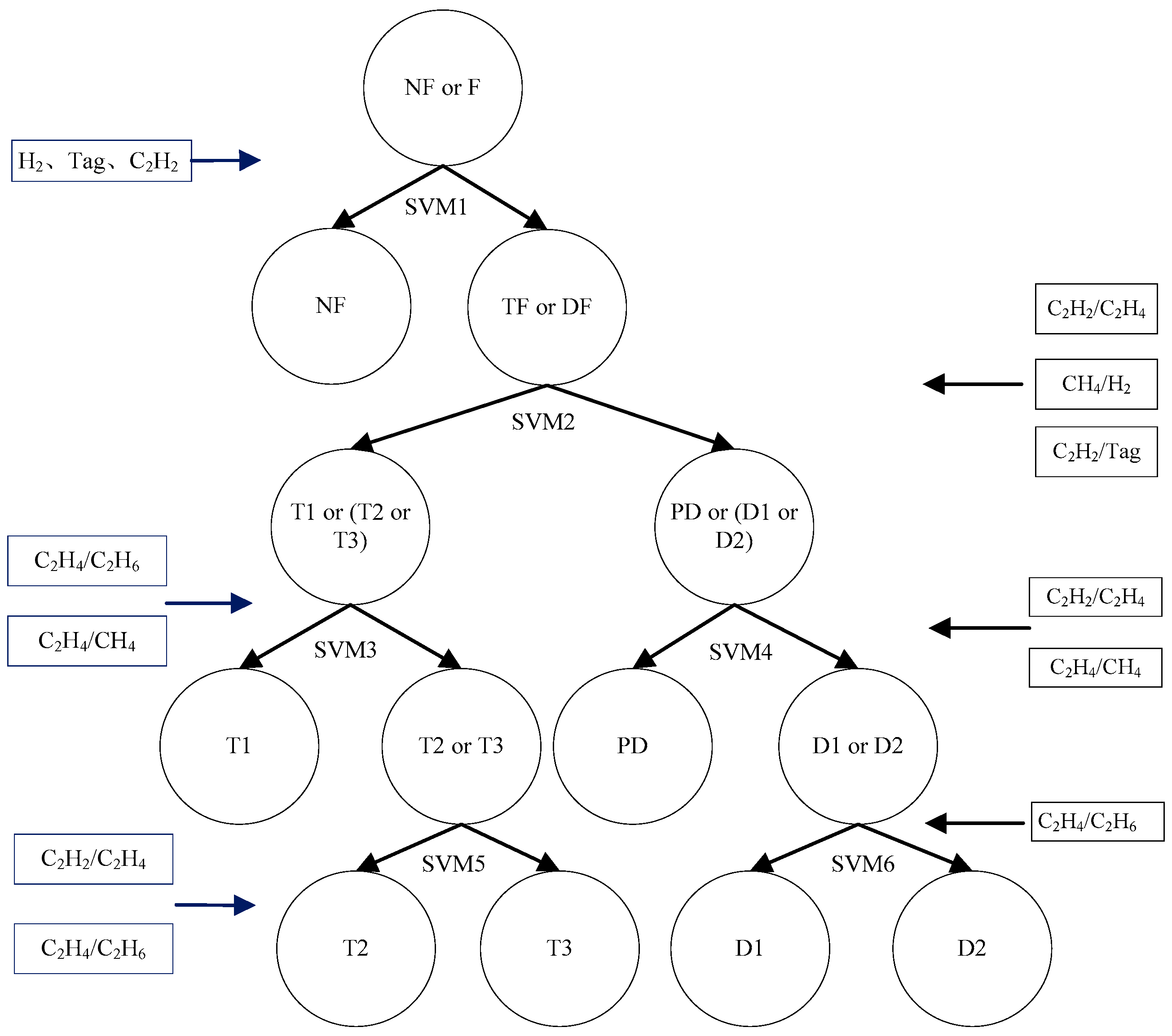
4.2. Model Construction

The transformer fault diagnosis model based on CRO-TWSVM is composed of TWSVMs, the fusion DGA parameters, and multiple classification structures of a partial binary tree (PBT), as shown in Figure 3.

Seven fault modes are identified if the normal state is included: normal NF, low overheat T1 (below 300℃), medium overheat T2 (300–700℃), high overheat T3 (over 700℃), partial discharge (PD), low-energy discharge (D1), and high-energy discharge (D2).

The model includes a total of six sub-classifiers. To improve training and diagnosis efficiencies, the input of each sub-classifier contains characteristic parameters that are most effective for identifying the faults for which the sub-classifier is designed.

In this model, six TWSVMs, eight characteristic parameters, and four layers of fault samples classification were established to identify seven patterns. In the first layer, TWSVM1 is used as a classifier to classify the samples into a normal sample (NF) and fault sample (TF and DF). In the second layer, TWSVM2 is used as a classifier to classify samples into discharge fault (DF) and overheat fault (TF). In the third layer, TWSVM3 and TWSVM4 are used. TWSVM3 is used to classify T1, T2, and T3; and TWSVM4 is used to classify PD, D1, and D2. TWSVM5 and SVM6 are used in the fourth layer for further fault classification. TWSVM5 is used as a classifier to classify the samples T2 and T3, TWSVM6 is used as a classifier to classify the samples D1 and D2.

5. Examples of the Transformer Fault Diagnosis Model

5.1. Diagnosis Examples

The training and test sample set used by CRO-TWSVM model included 960 pieces of data, part of the data in the sample set were actual 220 kV and 500 kV transformer DGA data taken from a provincial branch company of the state grid and some were raw DGA data taken from the literature [3,6,7,8,9,10,35,36,37,38,39]. Four hundred and fifty seven (457) pieces of data were extracted from the sample set, among which 345 pieces were taken as training samples and 112 pieces were taken as test samples. Meanwhile, PD and T3 samples are properly processed to achieve an ideal unbalanced situation. The distribution of samples are given in

Table 2. Training sample distribution table.

Fault Code	Training Sample (N)	Testing Sample (N)
NF	69	23
PD	28	17
D1	57	12
D2	51	21
T1	55	17
T2	58	10
T3	27	12
Total	345	112

.

The CRO-TWSVM fault diagnosis model was created on the MATLAB simulation platform. Parameters used to train the model are given in

Table 3. Training parameters of CRO-TWSVM fault diagnosis model.

Training Parameter	Paper
Number of input parameter	7
Number of classifiers	6
Range of c1	0.1–100
Range of c2	0.1–100
Range of q	0.1-30
kernel function	RBF
Epochs	4000
Goal of MSE	0.05
initial number of molecules	80
upper limit of KE loss	0.3
MoleColl	0.3
α	500
β	15
Iteration	7000
k-ford cross validation	5
Number of hidden unit	250

.

The training and testing result of the model are summarized in

Table 4. Training results of CRO model with 5-fold cross-validation.

Model	Training Sample (N)	Test Sample (N)	CRO
			Classification Accuracy (%)	C1	C2	q	Average Time (ms)
TWSVM1	345	112	98.21	47.23	2.67	8.21	5121
TWSVM2	276	89	98.88	59.12	16.43	21.66	4581
TWSVM3	140	39	97.43	22.36	46.92	3.09	3025
TWSVM4	136	50	94.00	57.13	8.54	5.47	3247
TWSVM5	85	22	90.91	2.76	10.68	18.73	1988
TWSVM6	108	33	96.97	71.55	12.08	10.02	2267

. The transformer fault diagnosis fusion model presented in this paper scores 94.64% in diagnosis accuracy and 308ms in diagnosis time, TWSVM4 and TWSVM5 is affected by unbalanced samples but also maintains high accuracy, therefore the fault diagnosis model presented in this paper not only offers a high diagnosis accuracy and a good generalization capacity but also consumes less time and is more efficient.

5.2. Random Test

As only one class of samples was tested in Section 5.1, there are contingency and subjective factors in the test. To ensure the objectivity and persuasiveness of the test, a random test was adopted and different random seeds were set in each test, so that the training set and test set generated by each sampling were different. The IEC, PSO-TWSVM, CRO-SVM, BPNN, random forest method (RF), Gradient Boosting Decision Tree (GBDT) and CRO-TWSVM models were selected for comparison. Meanwhile, considering that the data preprocessing may affect the performance of classifiers, CRO-TWSVM model without pre-processing is added for comparison.

The model was subjected to 10 random tests with 5-fold cross-validation, the test data are shown in

Table 5. Ten random tests of CRO-TWSVM with 5-fold cross-validation.

Test	Samples (N)	Training Samples (N)	Training Accuracy (%)	No. Test Samples	Testing Accuracy (%)
Random seed1	427	320	95.86%	107	94.61%
Random seed2	368	276	94.57%	92	94.57%
Random seed3	521	391	96.74%	130	95.97%
Random seed4	312	234	90.60%	78	88.46%
Random seed5	348	261	94.25%	87	94.25%
Random seed6	667	500	96.15%	167	95.95%
Random seed7	295	221	87.68%	74	85.42%
Random seed8	241	181	87.41%	60	87.97%
Random seed9	369	277	95.75%	92	89.97%
Random seed10	335	251	93.53%	84	94.33%

, and the 95% confidence interval (CI) of the diagnostic accuracy was calculated for comparison. The diagnostic results are shown in

Table 6. Comparison of 10 random tests.

Model	Testing Accuracy (%)			SD
	Average	Upper Limit	Lower Limit
PSO	90.84	93.8	87.88	2.96
SVM	88.71	92	85.42	3.29
BPNN	86.24	89.98	82.5	3.74
RF	86.83	90.18	83.48	3.35
GBDT	89.17	92.33	86.01	3.16
Without pre-processing	85.23	89.42	81.04	4.19
This paper	92.15	94.88	89.42	2.73

.

The comparison with the four models shows that: (1) The minimum and maximum sample size of 10 random test were 241 and 667. The 95% CI of the diagnostic accuracy of CRO-TWSVM was 89.42–94.88 and SD was 2.73 because the samples were picked at random and it’s hard to keep a balance. It’s worth noting that, in the case where the number of samples of random seed2, 4, 5, 9, 10 were close, and the test results were distributed between 89.97% and 94.33%, which further illustrates the impact of unbalanced samples on the test results; (2) RF, GBDT, SVM and TWSVM all show good generalization ability and robustness for transformer fault diagnosis. In terms of diagnostic accuracy, the order from low to high is RF, SVM, GBDT and TWSVM, respectively, and this is a very interesting phenomenon. Because in 10 random samples, there are different degrees of unbalanced samples, and the samples are kept to a small order of magnitude, in this case, RF does not give the best performance, more samples are needed to maintain better accuracy. Meanwhile, in the case of unbalanced samples, TWSVM is less affected than SVM and GBDT and shows better generalization ability; (3) the accuracy of the BP neural network was just 87.24% because producing highly accurate results with the BP neural network diagnosis method requires a large amount of sample data; (4) Compared with the model without pre-processing, the average diagnostic accuracy of the CRO-TWSVM model was improved by 6.92%; (5) the average diagnostic accuracy of the CRO-TWSVM and PSO-TWSVM model were similar, but the convergence rate was improved by 12.31%;(6) According to the comparison of the test results in Section 5.1 and Section 5.2, the test accuracy of CRO-TWSVM model was 94.46% in Section 5.1, while the range CRO-TWSVM under 95%CV was 89.42% to 94.88%, with an average accuracy of 92.15% in Section 5.2. This also shows that the method of random test can make the sample closer to the actual situation and maintain the objectivity of test results. Therefore, the CRO-TWSVM model described in this paper is better than other AI algorithms for fault classification and generalization and is more suitable for constructing a fault diagnosis model when few training samples are available.

6. Conclusions

This paper presented a transformer fault diagnosis model based on chemical reaction optimization and twin support vector machine. The following conclusions were reached following analysis and comparison of the diagnosis results produced by different models:

(1)

The proposed model not only combines the binary tree structure and TWSVM, but also integrates a variety of DGA parameters. On the basis of maintaining high diagnostic accuracy, training and diagnostic efficiency can be improved, and the problems of small sample size and unbalanced sample in transformer fault diagnosis can be solved. Our model’s application effect is better than the traditional IEC and Doernenburg ratio method, and is more suitable for transformer fault diagnosis than other AI methods. The tests showed that the model can be used for real-time diagnosis and analysis of power system equipment.

(2)

RBM was used for sample features optimization, and the random test method was adopted for test results optimization. The k-fold cross-validation method and the CRO method were used for hyperparameter tuning. These processes and optimization methods helped to considerably improve the generalization ability and robustness of the model. These methods are universal and can be used for reference in other models.

Our future work will focus on establishing a real-time fault diagnosis system to realize prediction and in-time diagnosis of transformer faults. The diagnosis system would decrease the working load of grid engineering and provide reasonable guidance for the management and maintenance of electrical equipment.