A Vibration Signal-Based Method for Fault Identification and Classification in Hydraulic Axial Piston Pumps

Abstract

In recent years, the interest of industry towards condition-based maintenance, substituting traditional time-based maintenance, is growing. Indeed, condition-based maintenance can increase the system uptime with a consequent economic advantage. In this paper, a solution to detect the health state of a variable displacement axial-piston pump based on vibration signals is proposed. The pump was tested on the test bench in different operating points, both in healthy and faulty conditions, the latter obtained by assembling damaged components in the pump. The vibration signals were acquired and exploited to extract features for fault identification. After the extraction, the obtained features were reduced to decrease the computational effort and used to train different types of classifiers. The classification algorithm that presents the greater accuracy with reduced features was identified. The analysis has also showed that using the time sampling raw signal, a satisfying accuracy could be obtained, which will permit onboard implementation. Results have shown the capability of the algorithm to identify which fault occurred in the system (fault identification) for each working condition. In future works, the classification algorithm will be implemented onboard to validate its effectiveness for the online identification of the typical incipient faults in axial-piston pumps.

1. Introduction

The online condition monitoring of components and systems is moving toward changing the paradigm in terms of maintenance, which is nowadays mainly founded on a time-based approach. The time-based maintenance acts in a preventive manner without considering the real state of the components. Scheduled inspections or substitutions are the fundamentals of the time-based approach, and therefore system downtimes could occur when not required, while a condition-based maintenance approach suggests action only when it is actually necessary. A well-scheduled condition-based maintenance depends on an efficient prognostics and health management (PHM) system in order to detect “if and when” maintenance is needed. In the last few years, the interest of the researchers in the PHM field has resulted in several industrial applications. The PHM can lead to significant advantages in terms of productivity, security, and reliability of the system. In the field of fluid power systems, PHM could be applied to circuits and components (valve, pumps, and motors), and it would become essential when interruption causes revenue losses, for instance in oil and gas plants and in chemical industries. Moreover, an unexpected failure can involve critical security issues, such as in the aircraft hydraulic systems [1,2]. This paper is focused on improving the reliability of a variable displacement pump used in hydraulic circuits by analyzing the potential of a PHM approach. Diagnostics and prognostics have different objectives: the former is aimed at identifying the health state of the system and is the first essential step for the latter, which tries to evaluate the remaining useful life (RUL) of the component. Diagnostic and prognostic processes can be developed with different methodologies that fall in two main categories: data-driven and model-based approaches [3].

The model-based method requires developing a complex mathematical model, able to replicate the functioning of the machine in both healthy and faulty conditions. However, in many cases, this task is very difficult to accomplish, therefore a data-driven approach is often preferred.

This paper is focused on the diagnostics that involve fault detection and fault identification (FDI), while prognostic issues are not yet considered, but are the final target of the research in progress. A data-driven approach is presented: it requires that sensors are installed on the systems to collect data that can contain the signature of the faults. In the field of fluid power systems, a few parameters can easily be monitored such as fluid pressure, fluid temperature, and vibrations. An important signal is the delivery pressure that can be utilized for developing effective diagnostic algorithms [4,5,6,7]. The pump delivery pressure can be measured through low-price sensors, but only faults involving the system fluid dynamics can be detected. In the field of hydraulic pumps, the literature reports other investigations: in particular, the measured fluid temperature was used for monitoring the overall efficiency of an external gear pump [8,9] and of a variable displacement axial-piston pump [10]. Other important signals, often used for diagnostics purpose, are vibrations measured by means of accelerometers; these signals can convey a lot of information about the health status of the system.

The literature reports some applications where the acceleration signals are used. In References [11,12], an internal combustion engine was monitored with acceleration sensors, and a lot of vibration sources were detected due to the motion of the internal components, combustion, and so on. In general, since all pieces of information are merged, a careful analysis is necessary to find reliable data. Also, diagnostics of bearings exploits vibration signals, as reported in References [13,14]. In some cases, vibrations appear when cavitation occurs, detecting abnormal working conditions in kinetic pumps [15,16]. In positive displacement pumps, an additional structure-borne noise is generated by the extremely high pressure oscillations in the delivery volume due to the back flow in conditions of incomplete filling of the variable chambers [17,18]. The characteristic mark of such a critical operating condition has been identified in the acceleration signals by Buono et al. [19] for a lubricating gerotor pump. Even the vibrations of hydraulic pumps can convey a lot of information about different faults; for this reason, many researchers have proposed diagnostics solutions based on an accelerometer installed on the case of the machine [20,21,22,23,24]. The methodology presented in Reference [25] is applied to experimental signals measured by two accelerometers mounted on the pump housing; the outcomes show that features highlighting the presence of the considered fault can be extracted by the proposed method for the analysis of the acceleration signals. Once a set of features sensible to the faults is extracted, it can be used to train an automatic algorithm whose purpose is to correlate the features to the faults. This automatic algorithm is used to perform a classification and is called a “classifier.” The classifier is trained offline and is then used online to compute the diagnosis. Many algorithms are presented in the literature for this classification task.

In many applications, a neural network (NN) is used as a classifier. The NN is a powerful tool that is used not only for diagnostics and prognostics, but also for many other tasks, as demonstrated in the review reported in Reference [26]. Other studies on condition monitoring exploit vibration signals for training NNs and to make the diagnosis [27,28,29]. Many examples of the application of NNs for the diagnostics of hydraulic circuits [30] and positive displacement pumps [31,32] are available.

Apart from the NN, many other algorithms are available for the classification task. Torrika [33] presented an interesting comparison of several algorithms for the case study of an axial-piston pump; in detail, a NN is compared to the following algorithms: naïve Bayes classifier, support vector machine (SVM), k nearest neighbor algorithm, and decision tree. In Reference [33], the higher classification rate is reached by the SVM. Another example of application of the SVM is presented in Reference [34] for the case study of a centrifugal pump. For the same component, in Reference [24], a decision tree algorithm was developed for the fault identification. An approach based on the use of a dynamic Bayesian network is presented in Reference [35] for the diagnostics, and also the prognostics, of a hydraulic circuit. In different studies [36,37,38], Helwig proposed the use of the Mahalanobis distance classifier for the diagnostics of hydraulic circuits. The same author also proposed the use of linear discriminant analysis (LDA) for the reduction of the number of features and the identification of the most relevant features to use as inputs of the classification algorithm. A theory worthy of note is the fuzzy logic. In References [7,21,39], the fuzzy logic is exploited to create inference systems for the fault classification. In many applications [31,40], the fuzzy logic is combined with the use of an NN for the classification task.

This paper reports the analysis of vibration signals acquired through two accelerometers installed on the pump case for identifying the health state of the pump. Tests were carried out, both in flawless and faulty conditions, where the faulty cases have been reproduced by intentionally assembling defective components into the pump. Vibration signals have been exploited to obtain the features used to train the classification algorithm where features reduction techniques and different classifiers have been evaluated to identify the best classification algorithm. The results show that it is possible not only to detect the faulty condition, but also to identify the type of fault.

2. Analysis Procedure

In this work, a vibration signal was used to evaluate the health state of the pump. A generic acceleration signal $x\left[n\right]$ could be decomposed in two main components particularly suitable for the further analysis, as shown in Equation (1):

$$x\left[n\right]=p\left[n\right]+r\left[n\right]$$

(1)

• $p\left[n\right]$ predictable part of the signal (CS1) the periodic part;
• $r\left[n\right]$ is the remaining noise containing all contributions not included in $p\left[n\right]$. This term can also incorporate CS2 contributions that are related to cyclic frequencies not contained in the periodic part CS1.

The CS1 and CS2 components are the most significant in acceleration signals, since usually, contributions at higher orders are negligible. In case of a gearbox [41,42], the contributions due to meshing of the gears are CS1, hence included in $p\left[n\right]$, while the contributions related to the ball bearings are CS2, therefore included in $r\left[n\right]$.

The Fourier spectrum can be used effectively for analyzing the periodic part of the signal, while the CS2 part can be analyzed with specific analytical tools such as spectral correlation density, cyclic modulation spectrum, and cyclic spectral coherence. In order to avoid misleading results, it is essential to extract the predictable part of the signal before analyzing the CS2 part [43].

The predictable term $p\left[n\right]$ is the periodic part (CS1) that corresponds to its expected value:

$$p\left[n\right]=E\left\{x\left[n\right]\right\}$$

(2)

The expected value operator $E$ refers to the ensemble average that is calculated by averaging diverse repetitions of the same stochastic process. The periodic part of the signal $x\left[n\right]$, can be computed through the operator $P$, which extracts all the periodic components of the signal under the hypothesis of cycloergodicity. For a cyclostationary and cycloergodic signal $x\left[n\right]$, the ensemble average is equivalent to the infinite cycle average [43]:

$$p\left[n\right]=E\left\{x\left[n\right]\right\}=P\left\{x\left[n\right]\right\}=\underset{K\to \infty }{\lim }\frac{1}{2K+1}{\displaystyle \sum }_{k=-K}^{K}x\left[n+kN\right]$$

(3)

with $N$ being the cycle length and $K$ the number of cycles. Equation (3) extracts only the periodic components that are multiples of the cycle, which, in turn, is known a priori. For rotating machines, like the hydraulic pump investigated, the basic cycle corresponds to one revolution of the shaft.

The method used for estimating the predictable part $\widehat{p}\left[n\right]$ is the synchronous average (SA) [43,44]. Assuming a signal $x\left[n\right]$ of finite-length L corresponding to $K$ cycles of $N$ samples each, the SA is given by Equation (4):

$$\widehat{p}\left[n\right]=E\left\{x\left[n\right]\right\}=\frac{1}{K}{\displaystyle \sum }_{k=0}^{K-1}x\left[m+kN\right]$$

(4)

The variable $m$ is reset at the end of every cycle and is limited in the range $\left[0,N-1\right]$:

$$m=n-\lfloor \frac{n}{N}\rfloor N$$

(5)

The SA is the cycle average calculated for a finite number of cycles. In the frequency domain, the expression is reported in Equation (6) [42]:

$$\widehat{p}\left[n\right]=E\left\{x\left[n\right]\right\}={\displaystyle \sum }_{k=0}^{\lceil N-1\rceil }{e}^{j2\pi knK/L}\frac{1}{L}{\displaystyle \sum }_{m=0}^{L-1}x\left[m\right]e^{-j2\pi kmK/L}$$

(6)

Equation (4) shows that the predictable parts are extracted at frequencies that are integer multiples of the cycle. As reported in Equations (4) and (6), the mathematical implementation of the SA requires a precise evaluation of the cycle length $N$ and that both $L$ and $K$ are integers; furthermore, in Equation (4), $N$ is an integer. When the samples come from an angular sampling, the conditions are all satisfied and $N$ is a known integer, since it depends on the acquisition system. Conversely, when angular sampling is not possible, resampling methods [44] can be applied to make $N$ an integer and to use Equation (4) for computing the SA, assuming available a sample per cycle to correct angular velocity fluctuations in the signal. Some limitations of resampling techniques, when a tachometric signal is not available, are presented in Reference [45]. Furthermore, in rotating machines, the angular velocity is often not exactly constant over the time; therefore, it could be impossible to resample starting from the time domain. Finally, an angular sampling, or an angular resampling (one sample per cycle), is needed for a suitable analysis of the signals.

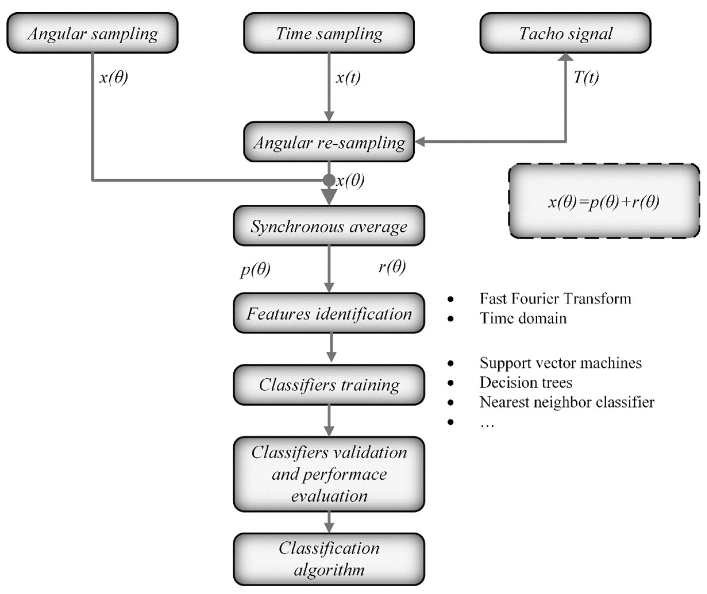
The proposed methodology decomposes the measured signal in several components that require analysis with apposite tools. Figure 1 illustrates a block diagram of the proposed procedure. The first step consists of acquiring an acceleration signal $x$ as a function of the shaft position $\theta$, where it is possible to obtain this signal with two different methods. With the technique used in this work, since a relative encoder was available, the signal $x\left(\theta \right)$ was directly obtained through an angular sampling. Figure 1 also reports an alternative approach that can be used if an encoder were not available. In this case, a time sampling of the acceleration signal $x\left(t\right)$ is performed, and subsequently, an angular resampling is necessary, but a tachometric signal T(t) is required.

The synchronous average $p\left(\theta \right)$ can be obtained with Equation (6) from the signal $x\left(\theta \right)$ in the angular domain. The SA contains the CS1 components of the signal and it can be analyzed with either the fast Fourier transform (FFT) or the Power Spectral Density (PSD) tools. The residual signal $r\left(\theta \right)$ is calculated by subtracting the Synchronous Average (SA) from the acceleration signal $x\left(\theta \right)$. The residual signal includes both the CS2 components and the higher order cyclostationary component, which can be analyzed with either FFT tools or other advanced methods, such as the spectral correlation density (SCD) or the cyclic spectral coherence (CSC). It is important to subtract the SA from the raw signal before analyzing the CS2 components, since the results of the CS2 analysis can be altered by the presence of periodic components. The residual signal contains also the background noise, which could make the results of the CS2 analysis less clear.

Once the components have been separated, the extraction of the features from the acceleration signal is carried out. After the feature reduction, the reduced features are used to train different classifiers and a distinct set of data is exploited to validate each classification algorithm. By evaluating the performance of each trained classifier, the best classification algorithm can be detected.

3. Experimental Activity

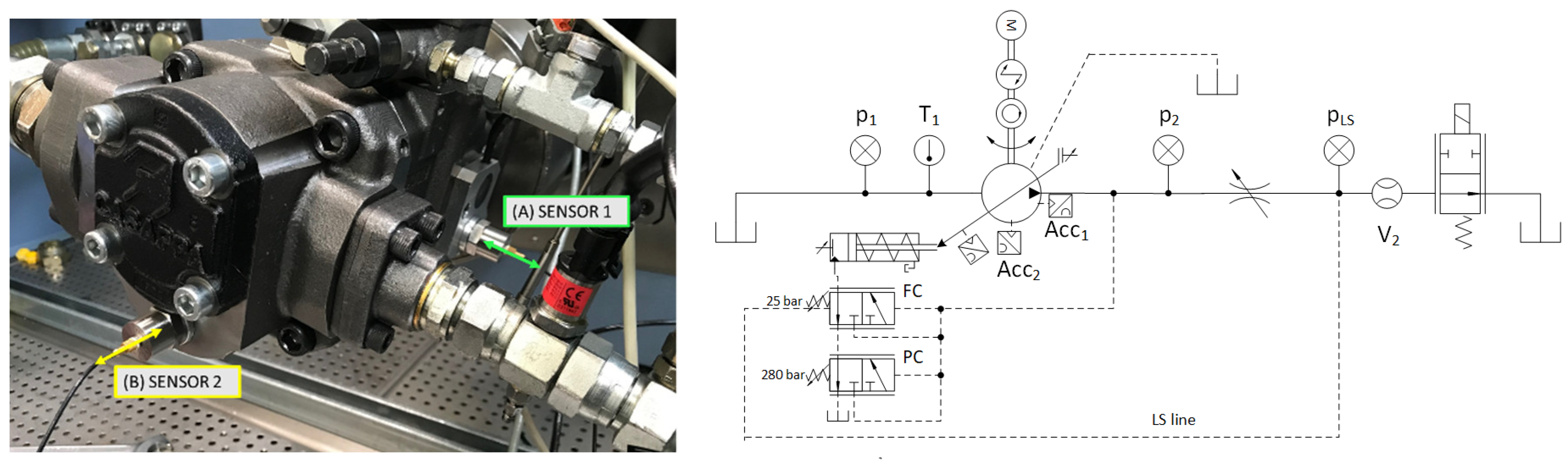
The research activity was supported using experimental tests carried out at the laboratory of the Engineering and Architectural Department of the University of Parma. A couple of accelerometers were installed on a pump that was tested in both healthy and faulty conditions for extracting suitable parameters for the diagnostics. Pictures of the tested pump (a) and of the experimental layout (b) are reported in Figure 2. The hydraulic pump was a swash plate axial-piston type with a maximum displacement of 84 cm³/rev, equipped with a hydro-mechanical load-sensing regulator.

Two piezoelectric accelerometers were installed on the pump housing, as shown in Figure 2a, and located in orthogonal directions for understanding which position provides the most meaningful information.

As illustrated in Figure 2a, one accelerometer (sensor 1) was mounted on the case for measuring the acceleration in the inlet–outlet flow direction. The second accelerometer (sensor 2) was applied on the pump cover for measuring the acceleration in the direction of the piston axes. Both sensors were piezoelectric charge accelerometers (Brüel & Kjær type 4370) with an accuracy of ±2 m/s² and a bandwidth up to 10 kHz that can measure a maximum continuous sinusoidal acceleration of 20,000 m/s². The acquisitions were performed by means of a relative encoder for the angular sampling. The angular resolution of the encoder (0.1 deg) led to high sampling frequencies (2000 r/min, 120,000 Hz), significantly higher than the frequency necessary to exploit the accelerometer’s bandwidth.

As reported in Section 5, the results obtained by the sensors were comparable, therefore only the graphs related to sensor 1 are reported throughout the paper because a future installation of the sensor in the position 1 could be more appropriate with respect to the position 2, where the sensor could be damaged by accidental collisions.

In order to investigate the methodological approach, tests in faulty and healthy conditions were carried out. The faulty ones were obtained by introducing damaged and worn components in the pump.

The following faults were analyzed:

• Fault 1: worn port plate (F1)
• Fault 2: port plate with cavitation erosion (F2)
• Fault 3: worn slippers (F3)
• Fault 4: cylinder block damaged on the contact surface with the port plate (F4).

All four conditions recreated faults that can occur in real applications. The selected faults were quite light since the objective of the present study was to exploit the proposed methodology for detecting incipient faults that could grow and lead to the complete failure of the pump. For confidential reasons, detailed information about the level of damage or worn could not be reported.

All faulty conditions were tested at a constant displacement of the pump (50 cm³/rev), equivalent to a swash plate angle of 12.8°, with different values of the delivery pressure and of the angular speed, as shown in

Table 1. Operating points considered for the acceleration acquisitions in healthy and faulty conditions.

Angular Velocity	Swash Angle	Delivery Pressure
		50 bar	150 bar	250 bar
500 r/min	12.8 deg	✓	✓	✓
1500 r/min	12.8 deg	✓	✓	✓
2000 r/min	12.8 deg	✓	✓	✓

.

For each acquisition, 90,000 samples, corresponding to 25 revolutions, were acquired. In order to have more data available for the classifier training phase, the tests were repeated 5 times for each operating condition. Since 9 operating conditions were considered, and each had been acquired 5 times, 45 different acquisitions were considered for each fault configuration.

4. Experimental Results

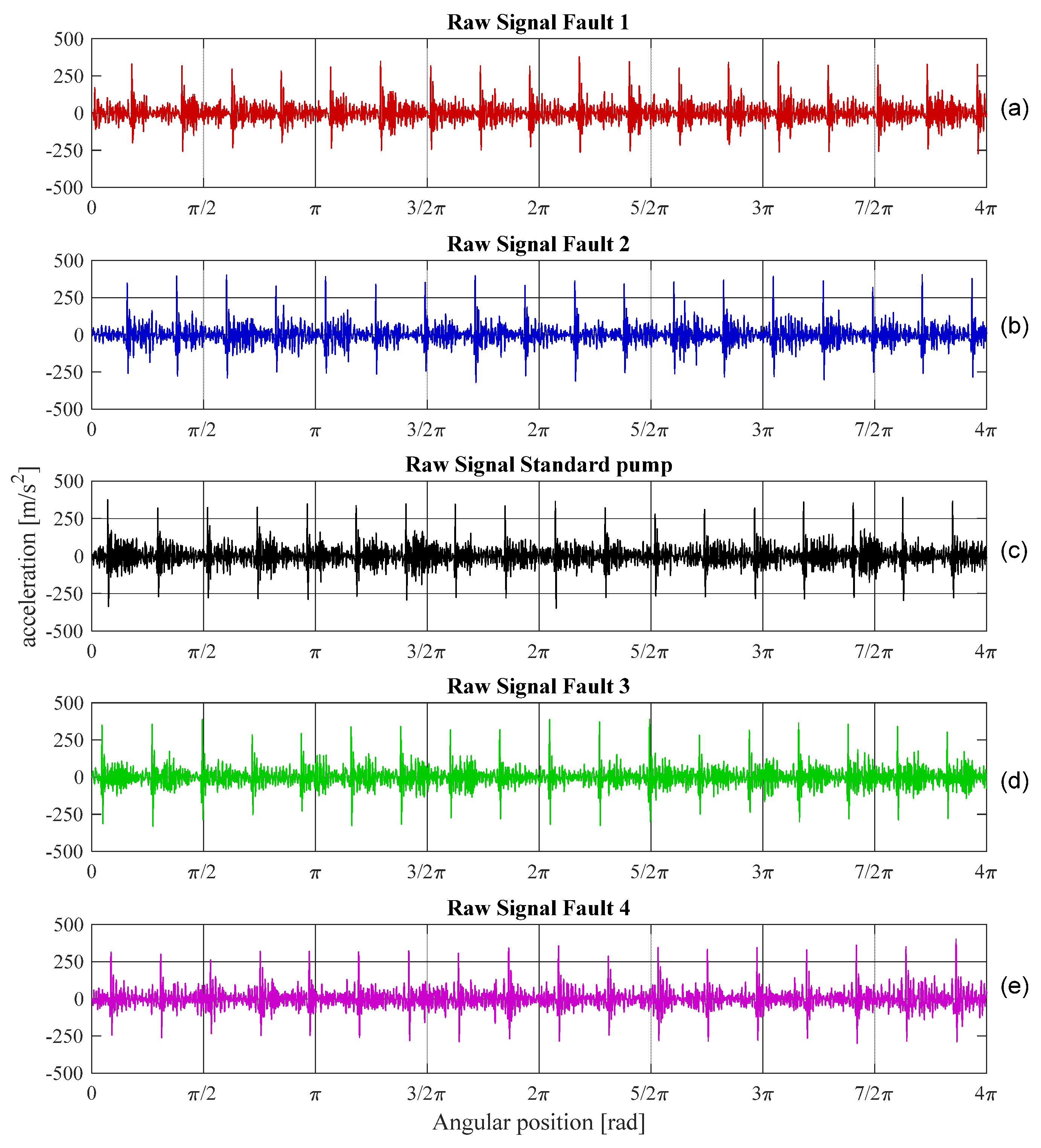
In this section, the procedure proposed for the decomposition of the signal that was applied to the acceleration signal acquired during the tests is described. The unit was tested in both healthy and faulty conditions and the final aim of the analysis was to extract relevant parameters for the pump diagnostics. Figure 3 reports the acceleration signals measured with sensor 1 in a healthy condition (standard pump) and in faulty condition, in a particular working condition (1500 r/min, 150 bar); all signals are plotted over a period of two revolutions (4π rad).

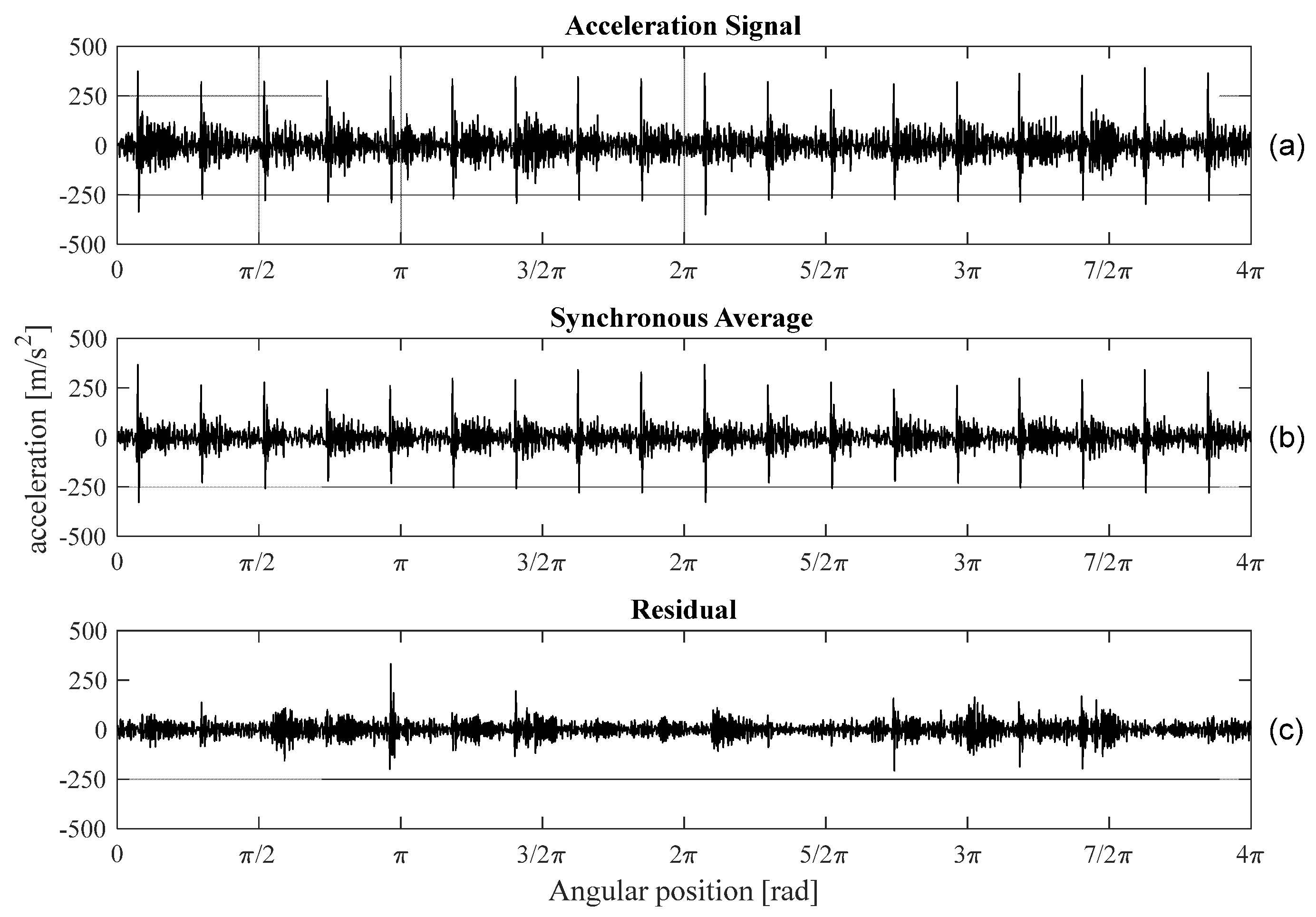
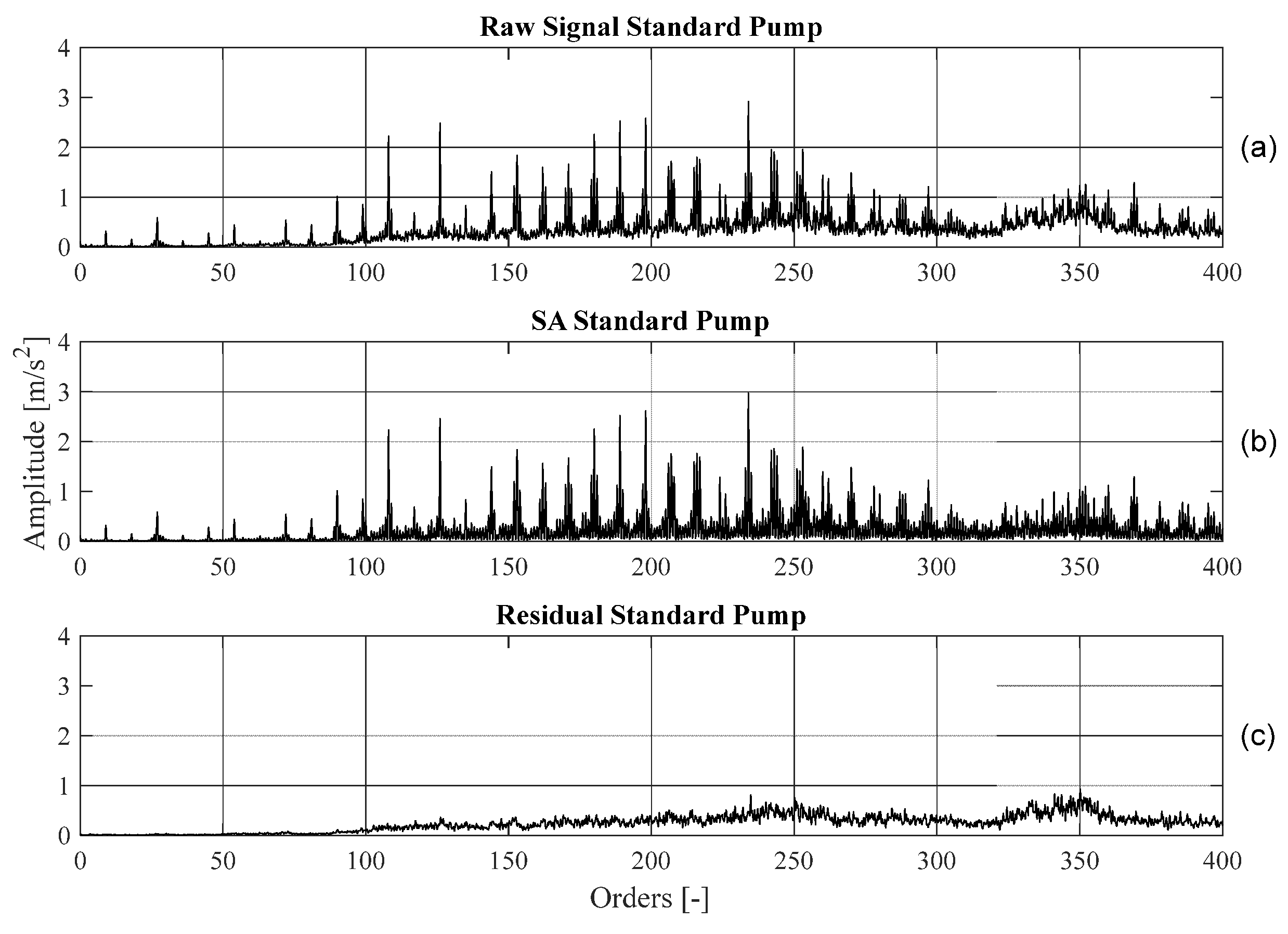
For each working condition tested, the raw signal was decomposed in two different contributions: the periodic part (SA) and the remaining noise (residual). The periodic part (SA) was extracted from the raw signal by considering 25 revolutions, while the residual part was calculated by subtracting the SA from the raw signal. Figure 4 shows how the signal acquired for the standard pump with sensor 1 in a specific working condition (1500 r/min, 150 bar) was decomposed.

The decomposition methodology was applied, both in healthy and faulty conditions, for each acquired test. In order to highlight the difference between the standard and faulty pump, the signal was processed in the frequency domain instead of in the angular domain. The extraction of features in the frequency domain was performed by separately computing the fast Fourier transform (FFT) of the considered signal (raw signal, SA, residual). The computation of the FFT returns many frequency features that can be used in the diagnostic algorithm; the considered features can be exploited to train a classifier. In this case, to train a classifier, the FFT coefficients were used as features. For each acquisition, obtained at different working conditions, the FFT coefficients for the raw signal, SA, and residual were calculated. Each FFT was composed of 13000 coefficients. Figure 5 shows the FFT of the acceleration signal, SA average, and residual signal for the acquisitions with sensor 1 in the case of a flawless pump (1500 r/min, 150 bar).

Figure 6 and Figure 7 report a comparison of the FFT of the raw signal for the different healthy and faulty condition.

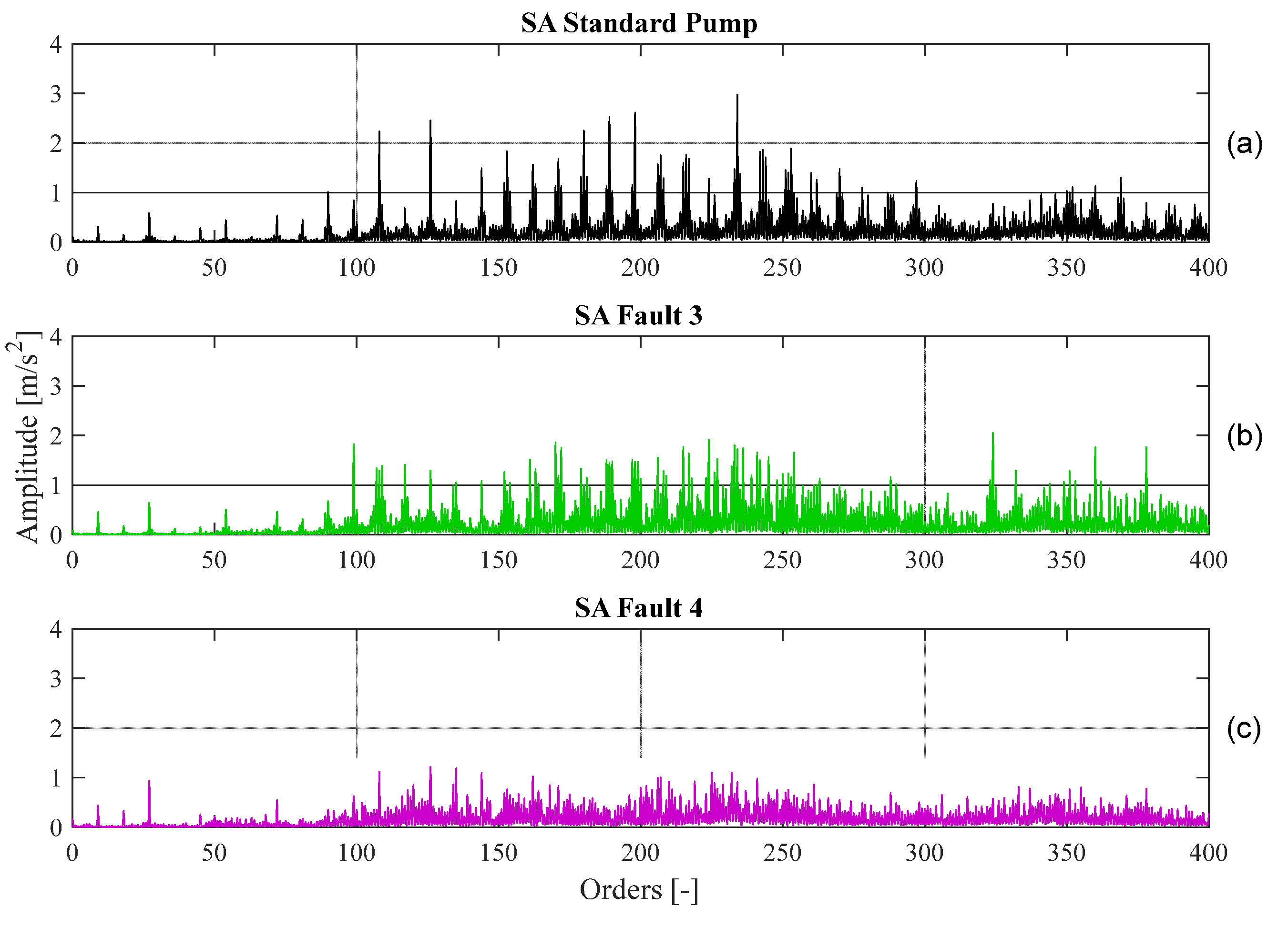
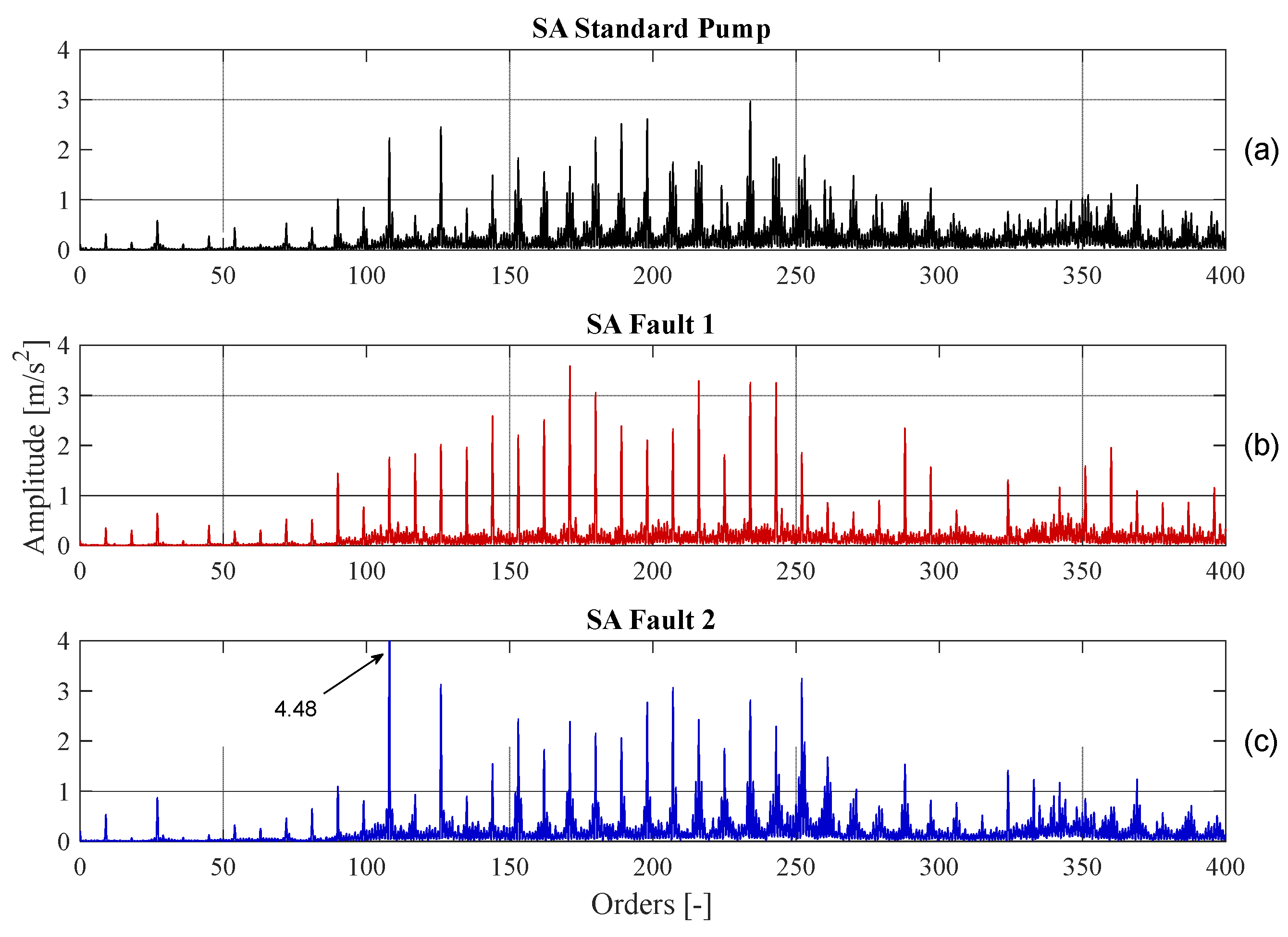
By observing Figure 6 and Figure 7, it is possible to notice how faults 1 and 2 present a similar trend with respect to the standard pump case, while faults 3 and 4 (Figure 7) show different trends. In particular, the FFT of the raw signals of faults 1 and 2 show repeatable peaks for multiples of nine, corresponding to the number of pistons. The FFT comparison of the synchronous average is also shown (Figure 8 and Figure 9) for evaluating the contribution of the periodic part of the acceleration signal.

Figure 8 and Figure 9 show that the spectrum of the SA signals and the obtained results are comparable to the cases calculated with the raw signal reported in Figure 6 and Figure 7. Therefore, it is difficult to highlight from the graphs significant advantages in using the FFT of the decomposed signal rather than the FFT of the raw signal.

In the following section, the FFT’s coefficients will be used as features to train various classifiers in order to verify whether the use of the decomposed signals with respect to the raw data improves the accuracy of classification for obtaining a reliable fault detection.

5. Classifier Comparison

The main aim of this paper is to detect the optimal solution for online condition monitoring in an axial piston pump, and consequently, to identify the best classification algorithm, the position of the accelerometer, and whether it is necessary to preprocess the acquired data.

Comparing a classifier performance on both the training set and the test set permits evaluation of the degree of generalization of the learning process. A wide range of different classifier types can be used for computing the diagnosis; in this work, a selection of seven classifiers were tested in order to find the optimal one.

Table 2. Different types of classifiers tested.

Classifier Category	Classifier
Decision Trees	Coarse tree
Discriminant Analysis	Linear discriminant
Ensemble Classifier	Bagged trees
K Nearest Neighbor Classifier	Weighted KNN Medium KNN
Support Vector Machine	Fine Gaussian SVM Linear SVM

shows the classifiers selected (right column) for the analysis and the category to which they belong. The classifier types used in this work were: decision trees, ensemble classifier, discriminant analysis, k nearest neighbor classifier (KNN), and support vector machine (SVM).

With the decision trees category, a tree structure is built for the classification models; in particular, a dataset is broken down into smaller and smaller subsets, while an associated decision tree is incrementally developed at the same time. The final outcome is a tree with decision and leaf nodes. The discriminant analysis classification method is grounded on the concept of finding a linear combination of predictors (variables) that best separates targets (classes). An ensemble classifier melds into one high-quality ensemble model the results coming from many weak learners, and qualities are a function of the algorithm choice. With the simple algorithm KNN, all available cases are stored and new cases based on a similarity measure are classified (e.g., distance functions). Finally, with SVM, the classification is performed by finding the hyperplane that maximizes the margin between the two classes; the vectors (cases) defining the hyperplane are the support vectors.

Typically, only one classifier was chosen for each classifier type, where exceptions include KNN and SVM with several kernel functions that have been considered twice [33].

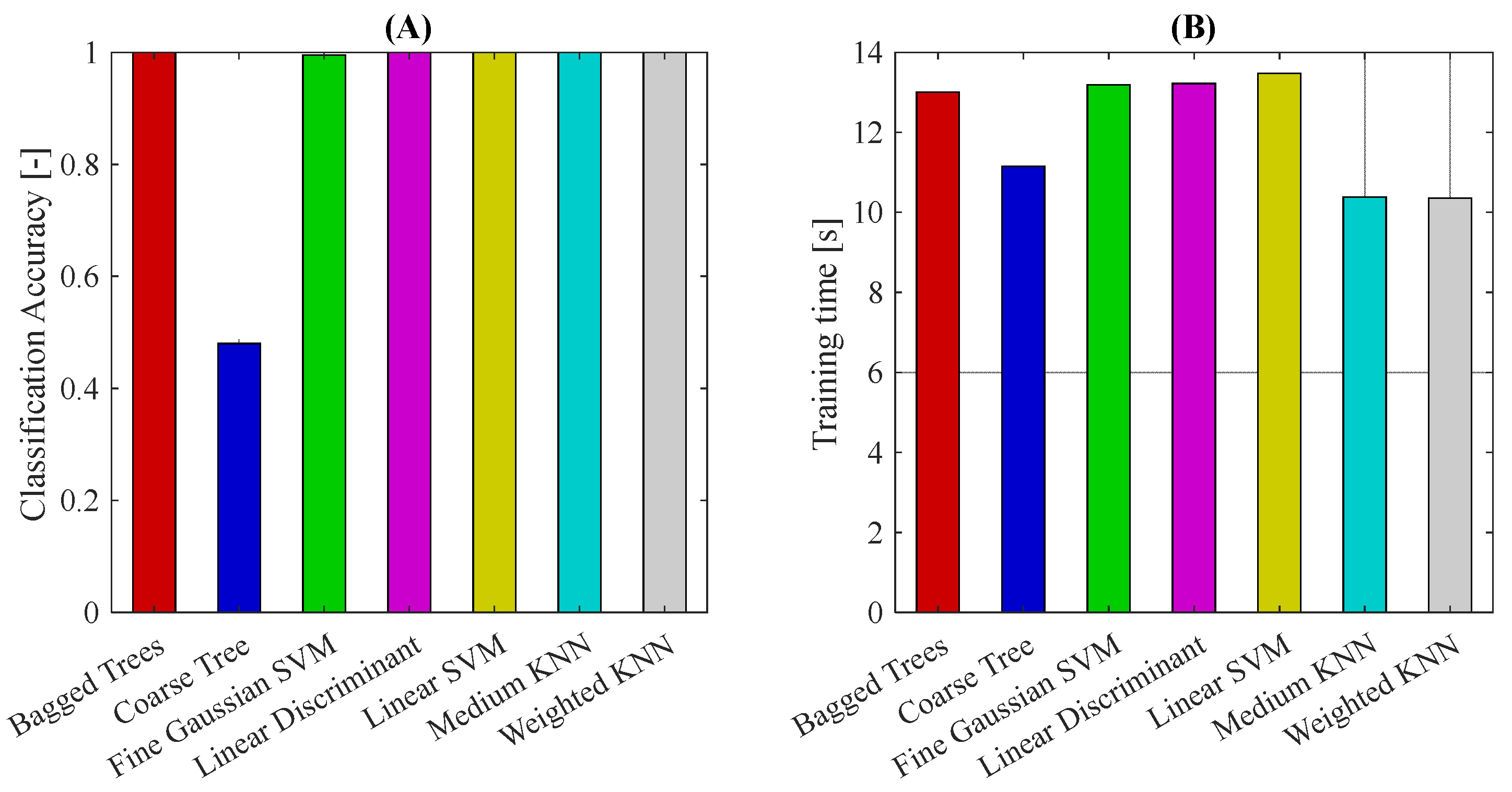
The first step was to compare the classification accuracy and training time for the different classification algorithms, considering as features all the FFT coefficients calculated in the orders domain (dimensionless frequencies). The classification accuracy was used as a synthetic parameter for evaluating the performance of a classifier [33]. Figure 10 shows the classification accuracy and training time obtained using all FFT coefficients for the raw signal for sensor 1 (13,000 features).

All the tested classifiers had a classification accuracy of 1, which means a percentage of 100% correct classification, except the coarse tree algorithm, which had a percentage of correct classification close to 50%. Besides, the training time was similar for the different classifiers except for medium KNN and weighted KNN. Both classifiers were nearest neighbor classifiers, which are algorithms that require less training time as they converge faster to the solution. These results are interesting but not suitable for online condition monitoring because they require a high run time and high memory space for saving data; therefore, it is necessary to reduce the number of features used for computing the diagnosis. A feature extraction phase was conducted by means of principal component analysis (PCA), obtaining 50 features instead of 13,000. PCA is a methodology employed for emphasizing variation and to bring out strong patterns in a dataset [46]. It is often used to make data easy to be explored and visualized. Once the features extraction had been carried out, the obtained features could be used to retrain the selection of different classifiers. 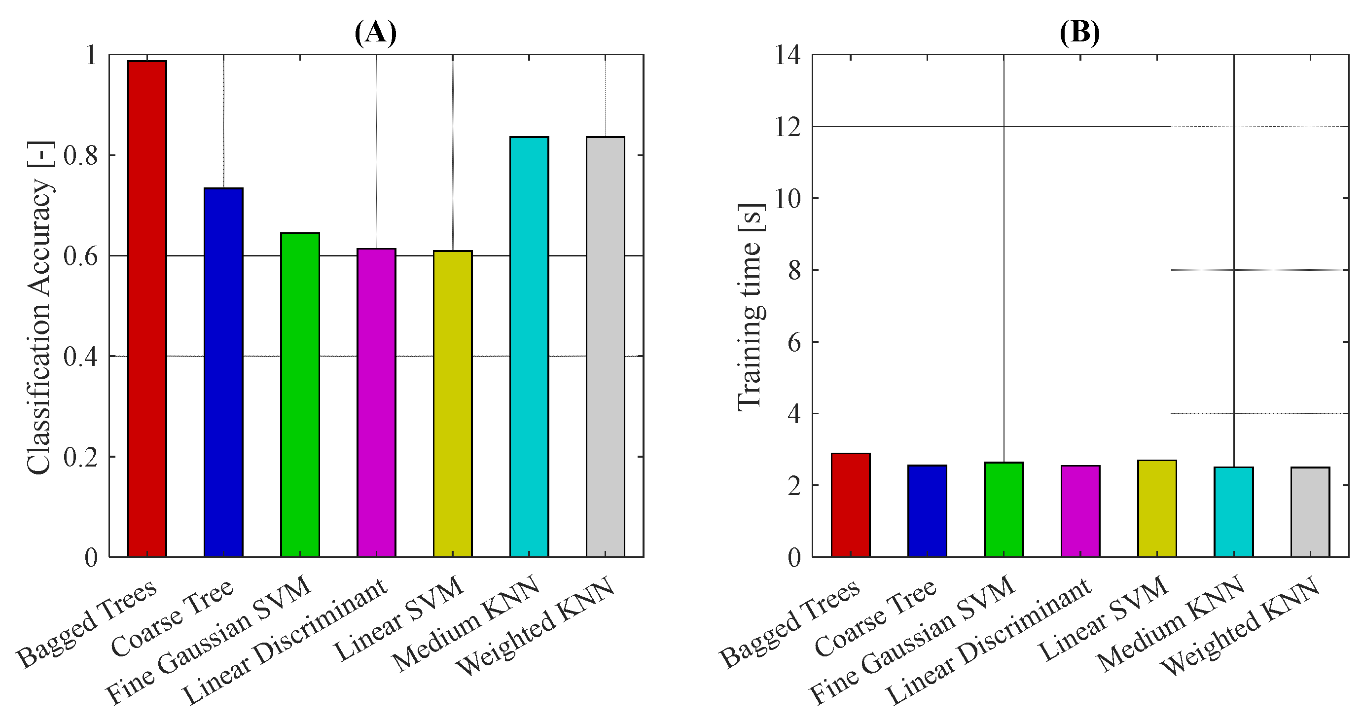Figure 11 reports the classification accuracy and training time for the raw signal considering only 50 main features.

Graphs reported in Figure 11 show a reduction in classification accuracy compared to the case without features reduction, with the exception of the bagged trees, and a training time reduction. In order to highlight where the algorithm failed to correctly identify the healthy condition of the pump, the confusion matrix (Figure 12) is shown for each different classification algorithm.

The classification accuracy is a synthetic parameter that allows for only evaluating the overall performance of the algorithm, but not to highlight the critical issues in classifying the data. These issues could be investigated with the confusion matrix.

The confusion matrix, also called error matrix, gives a representation of the accuracy of statistical classification. Each column of the matrix indicates the predicted class, while each row represents the real values. The confusion matrix associated with an N-class classifier is a square N×N matrix whose element A_ij represents the number (frequency, if normalized by the number of samples of class i) of patterns belonging to class i classified as belonging to class j. The name comes from the fact that shows whether two classes are confused (i.e., commonly mislabeling one for another).

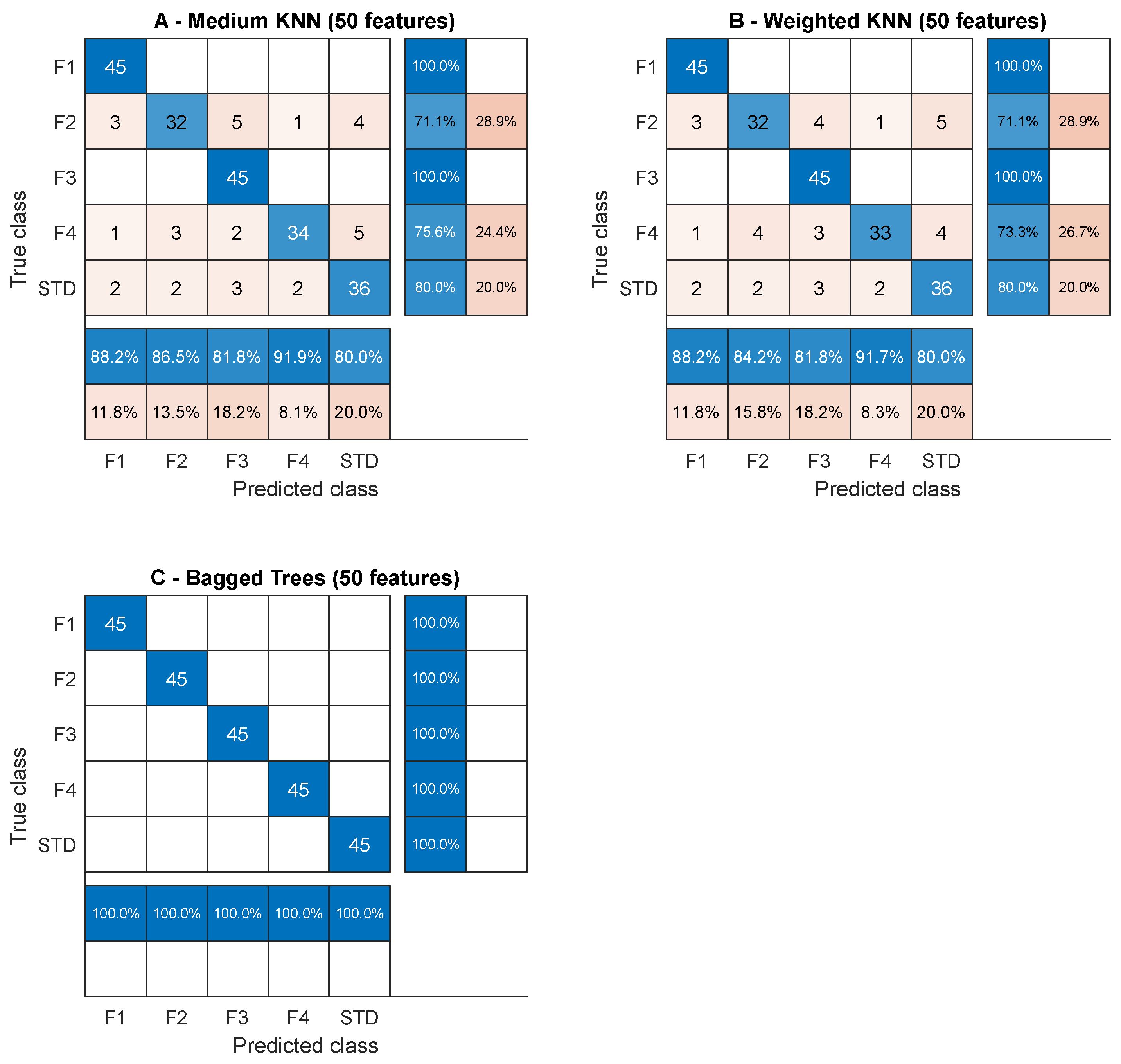
Figure 12 and Figure 13 show which classifiers make it possible to correctly classify the state of health of the machine. In particular, the confusion matrix allows for observing in detail which fault configurations are classified correctly. From the analysis of the matrices, significant considerations can be done. In general, fault 3 was the simplest to be detected, with the exception of the coarse tree (Figure 12A), with a success rate of only 66.7%. The linear SVM (Figure 12C) failed in identifying the fault 4 twice out of three times; moreover, there were many false alarms. Roughly, for all four algorithms in Figure 12, in 50% of the cases, they were not able to detect a failure condition. Fault 3 was always predicted correctly by all classifiers in Figure 13, but also fault 1 was likely to be detected. As already highlighted by the aggregated data in Figure 11a, the bagged tree (Figure 13C) is reliable.

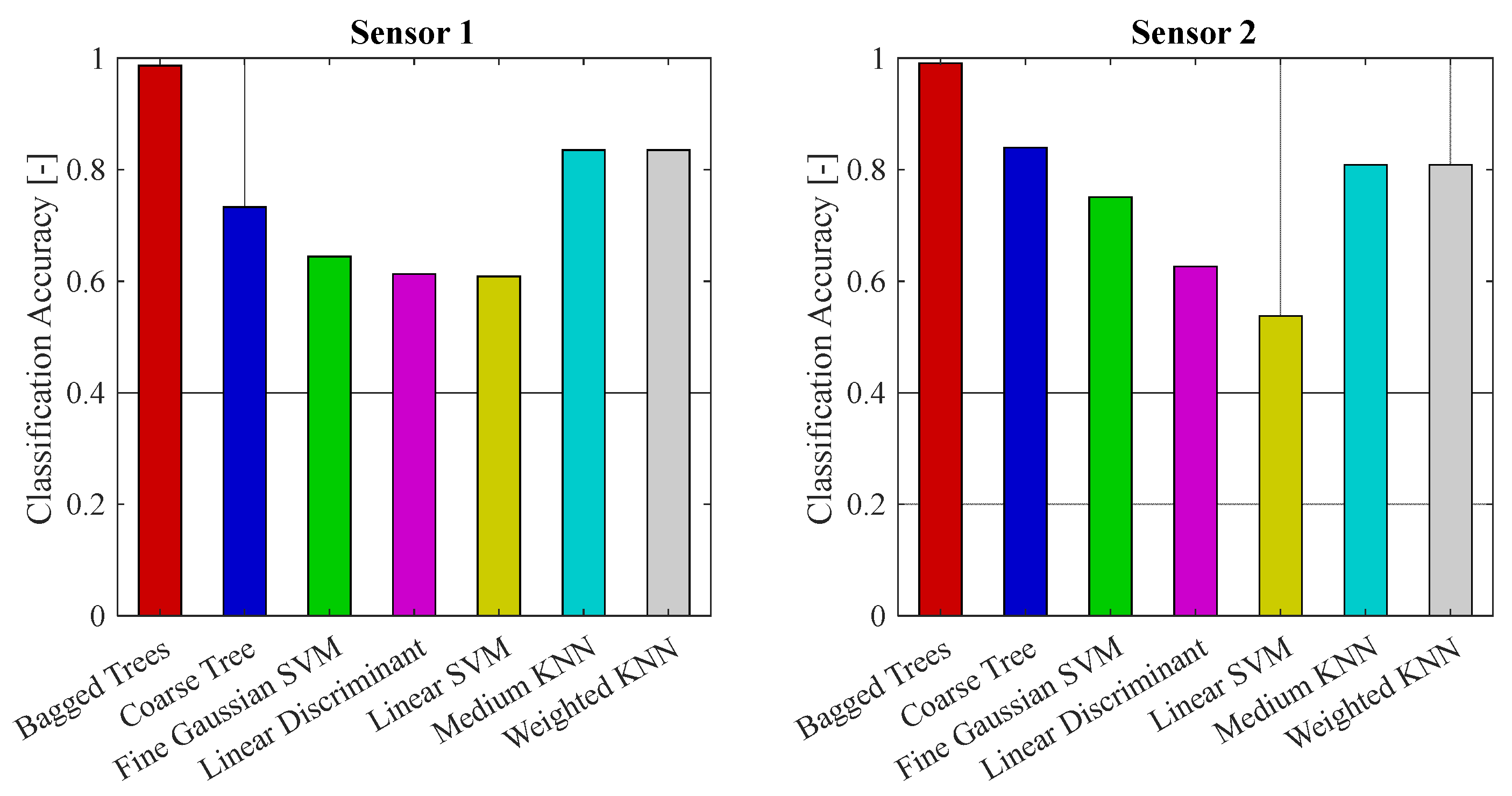
In order to compare the best position for connecting the accelerometer, the comparison between the classification accuracy for the two sensors is shown below.

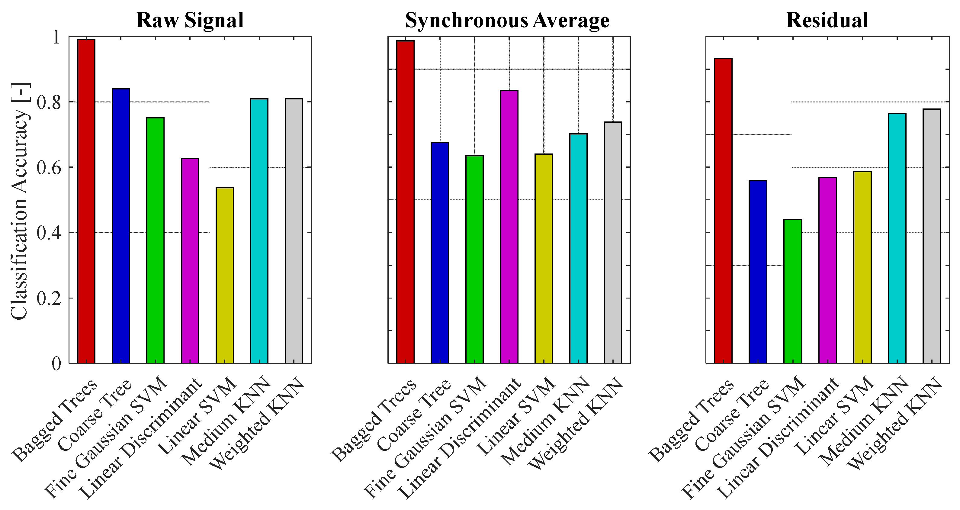
As already introduced, sensor 1 and sensor 2 were accelerometers with the same characteristics placed in different positions; sensor 1 was installed to measure the vibrations in the direction of the suction–delivery flow, while sensor 2 was put on the pump cover for measuring the acceleration in the direction of the shaft axis. The results obtained are comparable, as shown in Figure 14; therefore, the sensors positions can be considered equivalent. In the final analysis, the performance of the different classifiers with the variation of the features used for training the classification algorithm. In particular, with the analysis procedure presented in Section 2 the vibration signal (raw signal) acquired with angular sampling can be decomposed in two main contributions: synchronous average and residual signal. Each classifier has been trained using the 50 main components obtained through the PCA as features, starting from the FFT coefficients of each part of the acceleration signal.

The results shown in Figure 15 highlight a slightly higher classification accuracy in the case of a raw signal than the decomposed signals. This is a relevant result because it permits one to use the raw signal directly, avoiding the decomposition procedure of the signal itself.

Besides, the considered features were the coefficients of the FFT of the raw signal and they could be acquired either with time or angular sampling. A solution based on the time sampling of the acceleration signals without the decomposition is a relevant result because it will permit implementation in an onboard application.

The results reported in Figure 15 also show that the bagged trees was the classifier with the best performance; indeed, the classification accuracy for the bagged trees classifier was very close to 100% for all the cases analyzed.

6. Conclusions

The results presented in this paper show that it is possible to identify faulty conditions in an axial piston pump with classification algorithms exploiting vibration signals.

The paper presents a feature extraction using PCA techniques and different classification algorithms in order to find the best diagnostic approach. The FFT transform produced a big vector of coefficients (features) that provided classification accuracy close to 1 for each tested classifier.

A reduction of the features was necessary to reduce the computational effort for online condition monitoring. By decreasing the number of features, the classification accuracy was slightly lower for each classifier with respect to the case without features reduction; the bagged trees algorithm results showed it to be the classifier that presented the greatest accuracy with reduced features.

Using the reduced features, the analysis of the synchronous average and of the residuals did not present significant improvements compared to the analysis of the raw signal. Consequently, it is convenient to use the raw signal for a simpler onboard implementation. Furthermore, the raw signal could be acquired using time sampling, avoiding the use of an encoder; in fact, as described in the paper, angular sampling was required for the signal decomposition. The influence of the position of the accelerometers was also investigated by comparing the results obtained from two sensors installed in different positions. The comparison revealed that both sensors gave the same results, therefore both installation locations were functional for the diagnosis.

The achieved accuracy and robustness in test bench measurements will be further validated with measurements in an onboard application.