Sliding Mode-Based Robust Control for Piezoelectric Actuators with Inverse Dynamics Estimation

Abstract

This paper presents an improved control approach to be used for piezoelectric actuators. The proposed approach is based on sliding mode control with estimation perturbation (SMCPE) techniques. Also, a proportional–integral–derivative (PID)-type sliding surface is proposed for position tracking. The proposed approach has been studied and implemented in a commercial actuator. A model for the system is introduced, which includes the Bouc–Wen (BW) model to represent the hysteresis, and it is identified by means of the System Identification Toolbox in Matlab/Simulink. Experimental data show that the proposed controller has a better performance when compared to a proportional-integral (PI) controller or a conventional SMCPE in motion tracking. Furthermore, a sub-micrometer accuracy tracking can be obtained while compensating for the hysteresis effect.

1. Introduction

Piezoelectric actuators (PEAs) and micropositioning stages based on piezoelectric actuation are frequently used in a variety of applications where an ultrahigh precision motion is required [1]. They are used in micropositioning applications due to their characteristics, namely, high position resolution (nanometers or below), maximum blocking force (around hundreds of N), high stiffness, wide bandwidth, and very short response time. However, the nonlinear nature of the piezo-driven stages (typically suffering from drift, creep, and hysteresis) cause difficulties in its use in real applications. In particular, the hysteresis, which is the nonlinear relationship between the input (applied voltage) and output (displacement) that depends on both present and past inputs at the PEA, may induce a severe open-loop position error at the PEA which can reach as high as 10%–15% of the stage travel range. Therefore, in order to create high-precision PEA applications, the hysteresis should be compensated for. Creep, on the other hand, appears only in open-loop operations and could be eliminated by means of a closed-loop control strategy [2].

The successful compensation of hysteresis may be achieved by selecting adequate control strategies [3]. Frequently, hysteresis is compensated for by implementing a feedforward control that implements the inverse of any hysteresis model, such as the Preisach, Duhem, Maxwell, and Bouc–Wen (BW) models [4,5], or the Prandtl–Ishlinskii model [6]. However, since most hysteresis models are only applicable for some particular input signal frequencies, a combination of feedforward with feedback control is typically adopted for precision motion tracking [7].

Moreover, considering that modelling the hysteresis is a complex task, several approaches based on plant model identification without considering the hysteresis have been analyzed, based on different techniques such as PID (proportional–integral–derivative) control [8], H∞ robust control [9], inversion-based techniques [10], controllers based on linearized dynamic neural network models [11], or Pi–sigma fuzzy neural networks [12].

Another approach relies on considering the hysteresis as a disturbance or an uncertainty. In such cases, sliding mode control (SMC) techniques [13] have proven to be efficient and simple ways to deal with model imperfections and uncertainties for nonlinear systems [14,15]. SMC is an approach for controlling nonlinear systems by driving the trajectory of the state of the system onto a specified sliding surface and keeping it over this surface for the subsequent time. However, in conventional SMC design, the uncertainties must be bounded a priori. This typically yields to overconservative controllers, which may introduce two drawbacks: Poor tracking performance and undesirable oscillations in the control signal. Enhanced versions of the conventional SMC, aimed at overcoming these drawbacks, have been proposed, such as the adaptive sliding-mode position control in [16], or the so-called sliding mode control with perturbation estimation (SMCPE) in [17]. In this second improved version, the restriction of knowing the uncertainty bounds of the system is replaced by a strategy for estimating the perturbations online [17]. There are several implementations of SMCPE in the literature, for example in [18] for multiple frequency trajectory tracking or in [19] with a discrete reaching law with quasi-sliding-mode domains.

As described in [17], the existing SMCPE is featured with a proportional-derivative (PD)-type sliding surface and constant control gains. However, the commonly used PD sliding surface produces a slow response speed that may not be adequate for some systems. For that reason, an integral term was also introduced in the definition of the sliding variable [20]. As reported in [21], the traditional SMC with a PID sliding surface offers a faster transient response with a smaller steady-state error. Hence, SMC with a PID sliding surface has sometimes been adopted [22]. In this paper, a PID-type sliding surface has been introduced into the conventional SMCPE to establish a SMCPE–PID controller aimed at providing a faster transient response. This control scheme has been studied and implemented in a commercial actuator.

In the rest of the paper, the experimental setup of the piezoelectric actuator used is described in Section 2.1 and the dynamic model of the actuator with the Bouc–Wen hysteresis model is discussed in Section 2.2, including the voltage–displacement curve modelling and model parameter identification. Then, in Section 2.3, the design of a conventional SMCPE and an improved SMCPE controller with a PID sliding surface is developed, based on the model established before. Experimental studies are carried out later in Section 3, with the designed controllers and the results discussed. Finally, Section 4 contains the conclusions of the paper.

2. Materials and Methods

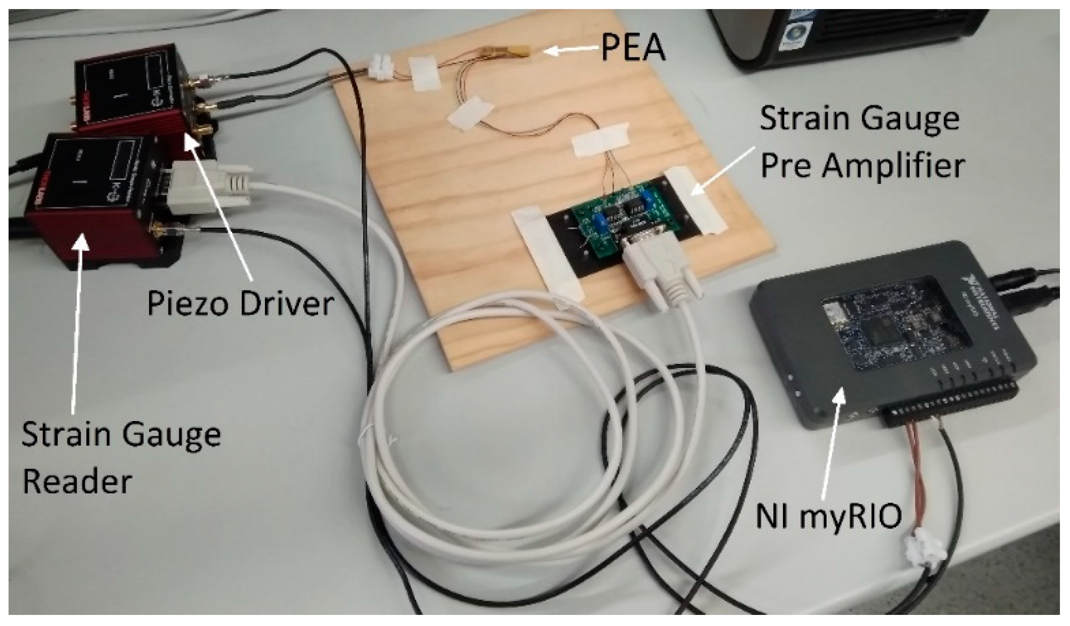
2.1. Experimental Setup

Commercial devices were used for the experiments in which the proposed controllers were implemented. The experimental setup for the PEA is shown in Figure 1. The commercial PEA (PK4FYC2 by Thorlabs), with a 38.5 µm range, was actuated within a 0–150 V range by the piezo driver (KPZ101 by Thorlabs). The driver was simultaneously controlled by the myRIO (by National Instruments), which functioned as the real-time controller, feeding the driver a 0–10 V control signal. The proposed SMCPE–PID controller, as well as the proportional-integral (PI) and conventional SMCPE controllers used for comparison, were all implemented with Labview, which was supported by the myRIO. The myRIO could work connected to a computer for easier monitorization and data acquisition of the control, or as a standalone controller. The displacement of the actuator was measured with a strain gauge integrated on it. The obtained displacement signal was amplified by the strain gauge pre-amplifier (AMP002 by Thorlabs) and the position of the actuator obtained with the strain gauge reader (KSG101 by Thorlabs) connected to it. The position of the PEA was then passed to the myRIO in a 0–10 V range to close the control loop.

2.2. Dynamic Modelling

Given that the performance of the motion tracking would be better when including the hysteresis model, since the system uncertainties would be smaller, the Bouc–Wen hysteresis model was considered. This model was used because it has few parameters and is quite easy to integrate with the rest of the model. Besides, it has already been verified that the Bouc–Wen model is suitable to describe the hysteresis loop of PEAs [23].

The dynamic model of the PEA with nonlinear hysteresis can be established as follows:

$$m\ddot{x}\left(t\right)+b\dot{x}\left(t\right)+kx\left(t\right)=k\left(du\left(t\right)-h\left(t\right)\right)+p\left(t\right)$$

(1)

$$\dot{h}\left(t\right)=\alpha d\dot{u}\left(t\right)-\beta \left|\dot{u}\left(t\right)\right| {\left|h\left(t\right)\right|}^{n-1} h\left(t\right)-\gamma \dot{u}\left(t\right){\left|h\left(t\right)\right|}^n$$

(2)

where the parameters m, b, k, and x indicate the mass, damping coefficient, stiffness, and displacement of the PEA, respectively. d is the piezoelectric coefficient, u represents the input voltage, and h denotes the hysteretic loop in terms of displacement where the magnitude and shape are determined by parameters α, β, γ, and the order n, where n governs the smoothness of the transition from the elastic to plastic responses. The piezoelectric coefficient indicates the relationship between the displacement of the PEA and the voltage applied to it. Usually, this relationship is a linear one, meaning d is a constant value: The relationship between the maximum displacement range and the maximum input voltage range (38.5 µm/150 V = 2.5667 × 10⁻⁷ m/V, in this case). But as seen in the hysteresis loop (Figure 2), the PEA used in the experiments does not behave linearly. Therefore, the relationship between the input voltage and displacement will need to be modelled, so this relation should be estimated experimentally for our piezo actuator.

For the elastic structure and material, n = 1 is assigned in (2) as usual. In addition, p indicates the overall perturbation of the system from model parameter uncertainties, unmodelled dynamics, and other unknown terms. These perturbations will be estimated later in Section 2.3.1.

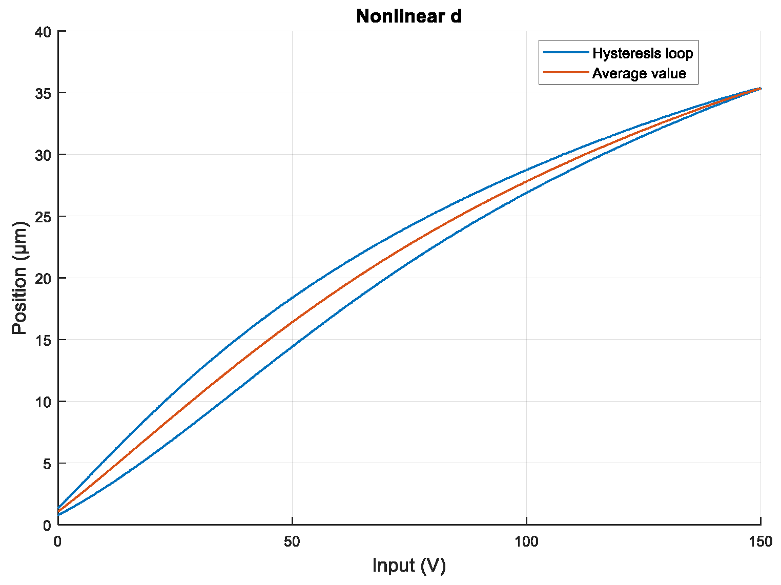
2.2.1. Voltage–Displacement Curve

As explained before, when the experimental validation has been carried out, it has been noticed that a nonlinear relationship exists between the applied input voltage and the displacement of the PEA. This nonlinearity is not related to the hysteresis, which, as seen in (1), only increases or decreases the displacement around the term $d·u$. Therefore, the relation between the voltage and the displacement d should be considered as a nonlinear term, and it was approximated as a curve consisting of the average of the values in the hysteresis loop, as shown in Figure 2. Using the Curve Fitting Toolbox by Matlab (R2017a), the curve was defined as $x=p_1\times u^3+p_2\times u^2+p_3\times u+p_4$, where p₁ = 1.553 × 10⁻¹³, p₂ = −8.621 × 10⁻¹⁰, p₃ = 3.567 × 10⁻⁷, and p₄ = 6.765 × 10⁻⁷.

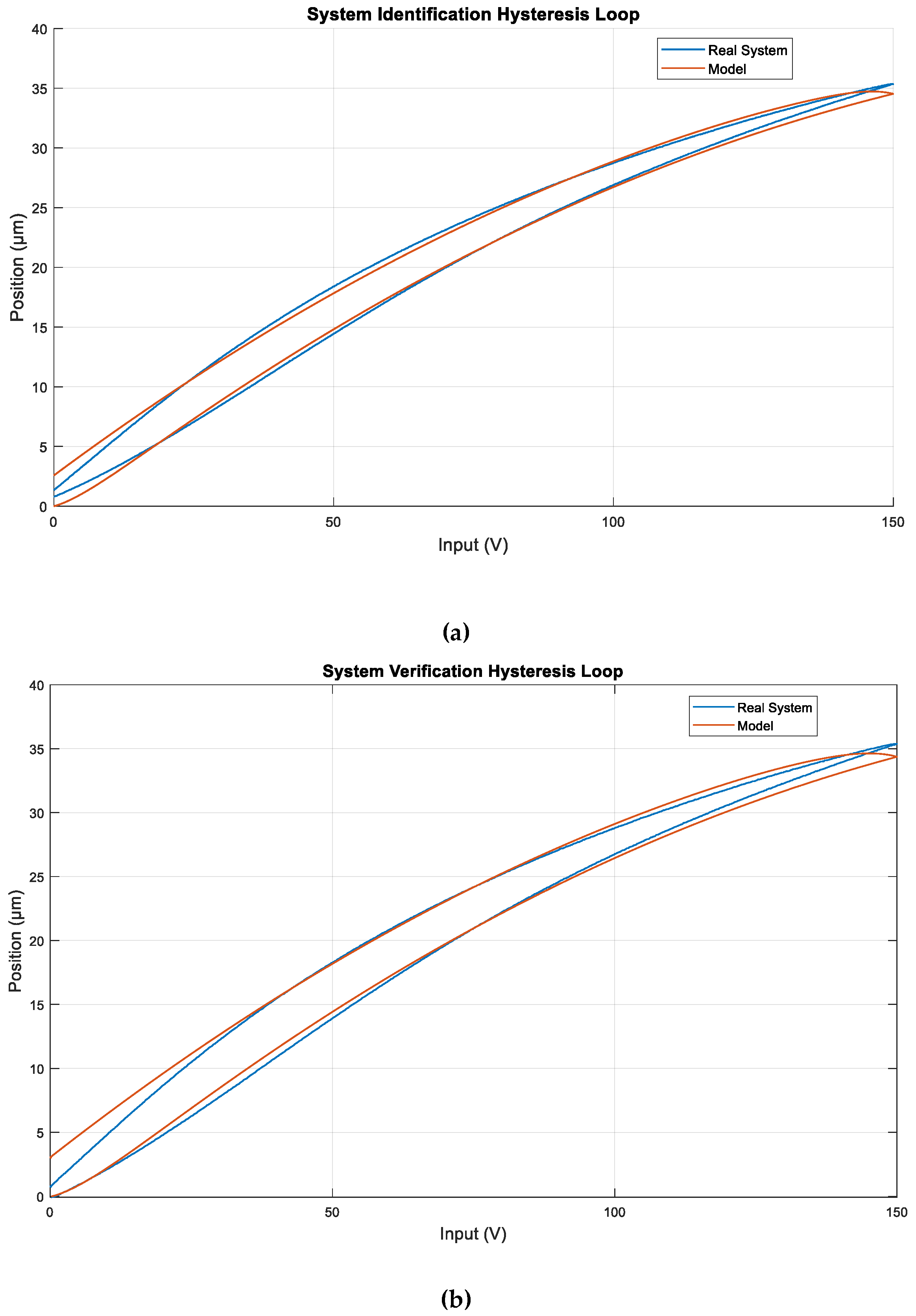
2.2.2. Model Identification with Parameter Estimation Toolbox for Matlab

The six other parameters m, b, k, α, β, and γ were identified simultaneously using the parameter estimation toolbox for Matlab/Simulink, using the nonlinear least squares method and Trust Region Reflective algorithm.

The model identification process was performed offline as follows:

• The experimental data for the model identification was obtained using three different input signals: Full-range (0–150 V) ramp, sinusoidal, and varying frequency sinusoidal signals, which will be described in Section 2.2.3.
• A dynamic model for simulating the PEA, which includes Bouc–Wen hysteresis, was implemented in Matlab/Simulink.
• The parameters were estimated for the simulation results to match the experimental data.
• Additional experimental data, also described in Section 2.2.3, was used for the verification of the model.

The results obtained for the parameters are displayed in

Table 1. Identified model parameters of the piezoelectric actuator (PEA) with BW hysteresis.

Parameter	Value	Unit
n	1
m	0.1343	kg
b	67.899	N s/m
k	262.78	N/m
α	0.0284
β	0.0207
γ	0.0727

. The resulting modelled hysteresis loop and the experimental loop are displayed in Figure 3, for the data used for identification and for the data used for verification.

2.2.3. Signal Description

Three different signals were used for the model identification. All three of them covered the whole 0–150 V range available in the actuator and lasted for 15 s. They were chosen for the identification because they were the signals expected to be used for future applications.

The signals were the following:

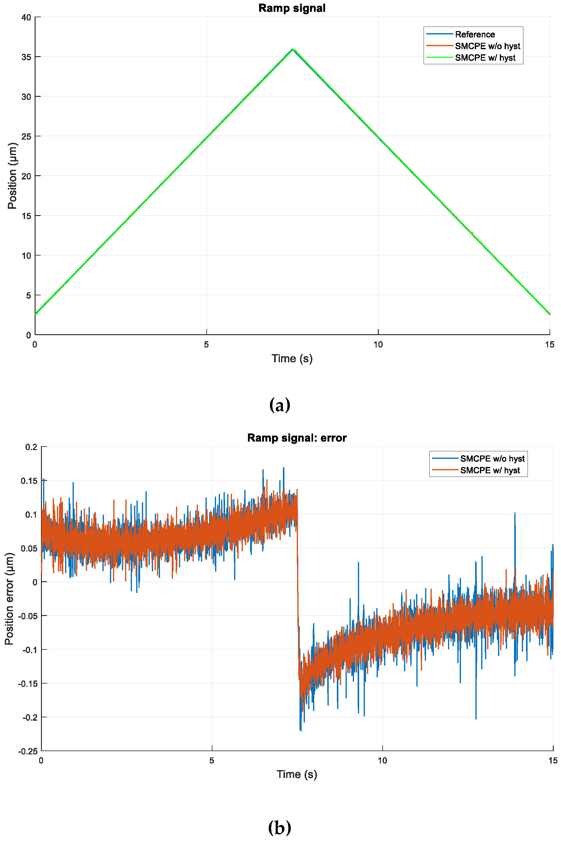
• The ramp signal for identification went from 0 to 150 V with a 20 V/s constant growth, and then back to 0 V with the same speed. For verification, it went from 0 to 150 V with a 40 V/s constant growth, then back to 0 V, back to 150 V, and finally back to 0 V, all with the same speed.
• The sinusoidal signal had a 75 V amplitude, 75 V offset, 0.2 Hz frequency, and −π/2 rad phase. For verification, it was the same signal but with a 0.4 Hz frequency.
• The varying frequency sinusoidal signal had 75 V amplitude, 75 V offset, −π/2 rad phase, and a frequency that went from 0.2 Hz and increased by 0.2 Hz after each cycle. No varying frequency sinusoidal signal was used for verification, since the identification data already covered a wide spectrum of frequencies.

2.3. Controller Design

The SMC technique is proposed in this work, due to its robust performance under model imperfections and uncertainties. Thus, this controller can compensate for both the errors in the model and other uncertainties. The next subsections describe the design of the conventional SMCPE and SMCPE–PID controllers for the PEA.

2.3.1. Conventional SMCPE

A perturbation estimation strategy already studied in the literature [4] was used, which resulted in estimating p as follows:

$$p_{est}\left(t\right)=m\ddot{x}\left(t\right)+b\dot{x}\left(t\right)+kx\left(t\right)-k\left[du\left(t-T\right)-h\left(t-T\right)\right]$$

(3)

Then, the system model (1) becomes:

$$m\ddot{x}\left(t\right)+b\dot{x}\left(t\right)+kx\left(t\right)=k\left[du\left(t-T\right)-h\left(t-T\right)\right]+p_{est}\left(t\right)+\tilde{p}\left(t\right)$$

(4)

where $\tilde{p}\left(t\right)=p\left(t\right)-p_{est}\left(t\right)$ represents the error between the system’s real perturbation and the estimated one.

To design the SMCPE controller, the position error was defined as:

$$e\left(t\right)=x\left(t\right)-x_d\left(t\right)$$

(5)

where x_d represents the position reference and t denotes the time variable. In the rest of this section, the time indices have been omitted for the sake of brevity of presentation.

As the dynamic system of the PEA is a second-order system, a first-order PD sliding surface was selected:

$$s=\dot{e}+\lambda e$$

(6)

where $\lambda$ ($\lambda$ > 0) is a design parameter.

The control law for the system (4), with sliding surface (6) and position error e given by (5), which satisfies $\underset{t\to \infty }{\lim }e\left(t\right)=0$ is the following, as proven in [4]:

$$u=\frac{m}{kd}\left(\frac{b}{m}-\lambda \right)\dot{x}+\frac{1}{d}\left(x+h\right)-\frac{1}{kd}{p}_{est}+\frac{m}{kd}\left({\ddot{x}}_d+\lambda {\dot{x}}_d\right)-\eta sgn\left(s\right)$$

(7)

where $\eta$ is a positive switching gain and sgn(s) represents the signum function, as defined in (8):

$$sgn\left(s\right)=\{\begin{array}{c}-1, for s<0\\ 0, for s=0\\ 1, for s>0\end{array}$$

(8)

Due to the discontinuity of the sign function, the control input may have chattering. To reduce this phenomenon, the boundary layer technique was used by replacing the signum function in (7) with a saturation function as follows:

$$sat\left(s\right)=\{\begin{array}{c}sgn\left(s\right), for \left|s\right|>\delta \\ s/\delta , for\left|s\right|\le \delta \end{array}$$

(9)

where the positive constant $\delta$ represents the boundary layer thickness, which makes sure that s is always bounded by $\delta$. When selecting parameter $\delta$, a tradeoff between chattering and tracking error should be taken. The control gain η depends on the upper bound of the perturbation error, and is usually tuned experimentally, since there is no universal method yet.

2.3.2. Improved SMCPE

In this section, an improved SMCPE with a PID-type sliding surface is designed.

In order to design an improved SMCPE controller, the following PID-type sliding surface was defined:

$$s\left(t\right)=\dot{e}\left(t\right)+{\lambda }_{1}e\left(t\right)+{\lambda }_2{{\displaystyle \int }}_0^{t}e\left(\tau \right)d\tau$$

(10)

where the error is described by (5), and ${\lambda }_1$ and ${\lambda }_2$ are design parameters and positive constants. These control gains should be selected so the characteristic polynomial $s^2+{\lambda }_{1}s+{\lambda }_2=0$ is strictly Hurwitz, i.e., a polynomial with roots located strictly in the left half of the complex plane. This condition ensures that e(t) tends to zero once the system reaches the sliding surface s(t) = 0.

The control law for the system (4), with sliding surface (10) and position error e given by (5), which satisfies $\underset{t\to \infty }{\lim }e\left(t\right)=0$ is the following, as proven in [4]:

$$u=\frac{m}{kd}\left(\frac{b}{m}-{\lambda }_1\right)\dot{x}+\frac{m}{kd}\left(\frac{k}{m}-{\lambda }_2\right)x+\frac{1}{d}h-\frac{1}{kd}{p}_{est}+\frac{m}{kd}\left({\ddot{x}}_d+{\lambda }_1{\dot{x}}_d+{\lambda }_2{x}_d\right)-\eta sgn\left(s\right)$$

(11)

where $\eta$ is a positive switching gain, sgn(s) represents the signum function, and the time indices have been omitted for the sake of brevity of presentation.

As stated before, the effect of the chattering was reduced by substituting the signum function in (11) with the saturation function in (9).

Furthermore, replacing (3) into the control law (11) yielded the following:

$$u\left(t\right)=u\left(t-T\right)+\frac{1}{d}\left[h\left(t\right)-h\left(t-T\right)\right]-\eta sat\left(s\left(t\right)\right)-\frac{m}{kd}\left[\ddot{e}\left(t\right)+{\lambda }_1\dot{e}\left(t\right)+{\lambda }_{2}e\left(t\right)\right]$$

(12)

The values for the controllers were obtained experimentally, since the parameters of the controllers could not be calculated analytically given that the system was not linear. These values are displayed in

Table 2. Values of the parameters of the controllers.

Controller.	Parameter	Value
PI	Kp	1
	Ki	0.001
SMCPE	λ	1000
	η	25
	δ	0.01
SMCPE w/PID sliding surface	λ1	450
	λ2	300
	η	0.5
	δ	18

. Several iterations were done in order to adequately tune the controllers’ parameters.

In the experiments, the values for the controllers’ parameters were experimentally tuned, taking into account the influence of these parameters in the controller performance. In the selection of these parameters, the following rules should be taken into account [24]. An increase in parameter η results in an increase in the absolute value of the control signal, but also increases the oscillation of the signal. This implies that an increment in η results in an increment in the system response speed and in the compensation of the uncertainties, but unfortunately also implies more activity control and more chattering that are undesirable in a real applications. On the other hand, the values of λ, λ₁, and λ₂ are related to the speed of the error convergence to zero when the system reaches the sliding surface. For example, an increment in λ implies an increment in the error convergence speed to zero, but also implies a bigger increase of the initial value of the sliding variable $s\left(0\right)=\dot{e}\left(0\right)+\mathsf{\lambda }e\left(0\right)$. Finally, an increment of the control parameter $\delta$ reduces the chattering but also increases the tracking error.

The performances of the SMCPE and SMCPE–PID controllers designed above were verified by experimental studies conducted in the subsequent section.

3. Experimental Results

Several experiments were carried out in order to ensure the designed controllers for the PEA offered a better performance than the usual ones. The performance of a PI controller was taken as a baseline and its performance was first compared to the conventional SMCPE. Then, the conventional SMCPE and SMCPE–PID were compared. Some tests were also carried out using the sliding mode controller without taking into account the effect of the hysteresis, to observe the improving effect the inverse hysteresis model had in the control of the PEA.

The signals used for these experiments were a ramp signal and a sinusoidal signal. They were similar to the ones described in Section 2.2.3, but in this case the signal range used for the experiments was 10–140 V, instead of the full 0–150 V range the PEA offers. This range was more than enough for application purposes, since it only reduced by 13.33% the 38.5 µm displacement range on the actuator, and prevented having any issues with controllability in the endpoints of the range. When moving the PEA to the endpoints of the working range, the control signal usually surpasses these borders in order to obtain a faster response, but as the input voltage was limited to the 0–150 V range, the control signal was smaller than it should have been, causing a very slow response.

Finally, the graphs displayed correspond to the position output and position error to visualize the behavior of the system, the control signal to understand how the controllers work, and the resulting position–reference graphs to easily visually compare with the open-loop hysteresis graphs and verify that the hysteresis effect was eliminated. The integral of the absolute magnitude of the error (IAE) performance indicator was also calculated and analyzed in order to compare the control qualities of the different controllers. Note that the displacement error of the PEA is in micrometers, hence the low values of the IAE performance indicator for the different controllers and reference types.

3.1. Comparison of the SMCPE with and without Hysteresis

First, the effect of the hysteresis in the SMCPE controller was studied to highlight the importance a good inverse hysteresis model can have in the performance of the control system. This was done by utilizing the sliding mode controller in (7) without taking into account the effect of the hysteresis (h), and comparing its results to the ones obtained with a SMCPE controller with the hysteresis as feedback.

A ramp signal was used to test the controllers, generating a reference that went from 10 to 140 V with a 17.33 V/s constant growth, and then back to 10 V with the same speed. This translates to a 2.57–35.93 µm range. The obtained error is seen in Figure 4b. The average errors were very similar in both cases, but when the hysteresis was ignored, the variations in the error were much higher. As the hysteresis was not considered when estimating the perturbation, the results given by the controller were worse, as the hysteresis still happened and was not considered.

The sudden change in the error at 7.5 s came from the change in the reference, as seen in Figure 4a. The displacement speed reference presented a step change from a positive to a negative value. Obviously, the real displacement speed could not track this step change in the speed due to the system inertia, and this delay was the cause of the step that appeared in the position error.

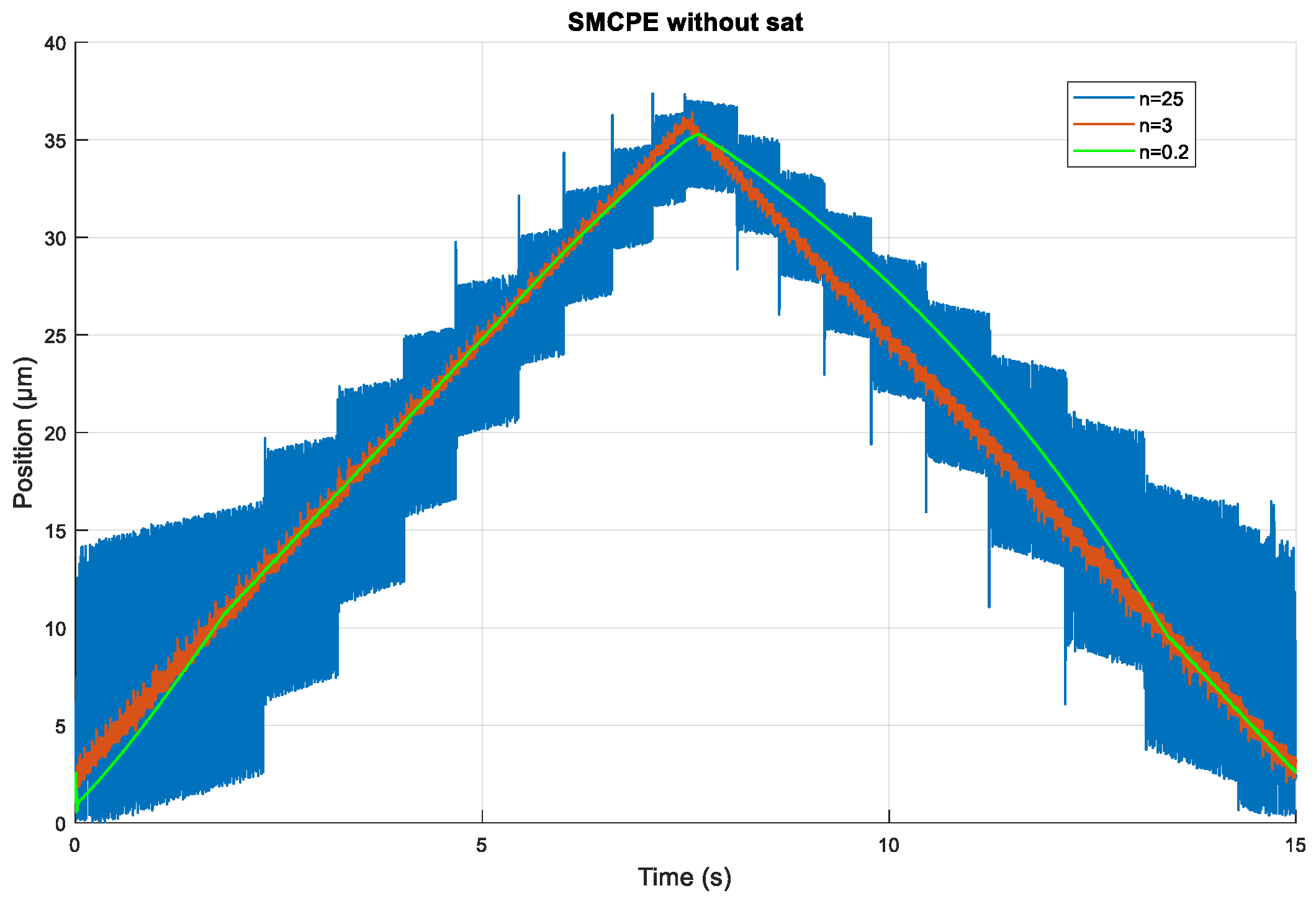
3.2. Comparison of the SMCPE with and without the Saturation Function

As mentioned in Section 2.3.1, saturation function (9) replaces signum function (8) in the control equation (7) in order to reduce chattering in the output. In Figure 5, the response of the system for the ramp signal defined in Section 3.1 is shown, when the saturation function was not implemented in (7).

The value used for the original SMCPE was η = 25, as seen in Table 2, and resulted in a very high-amplitude chattering. Reducing η made the amplitude in the chattering smaller, as seen with η = 3, but it was still present. However, reducing η too much (η = 0.2) will end up making the control signal insufficient, resulting in a worse system response, as seen when the reference changes, with a reduction in the compensation of uncertainties [24,25,26].

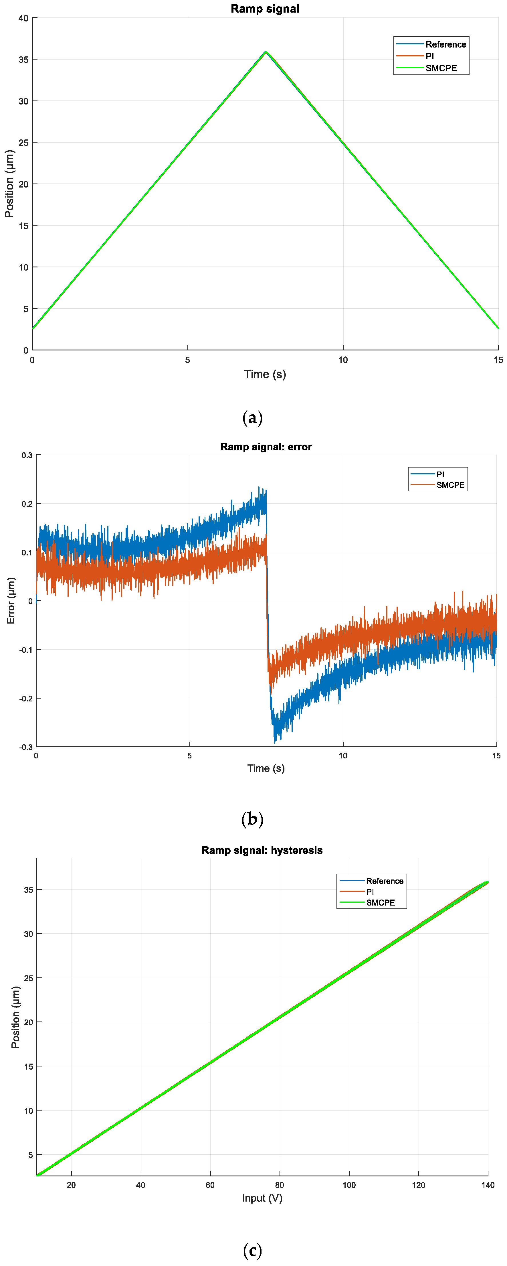
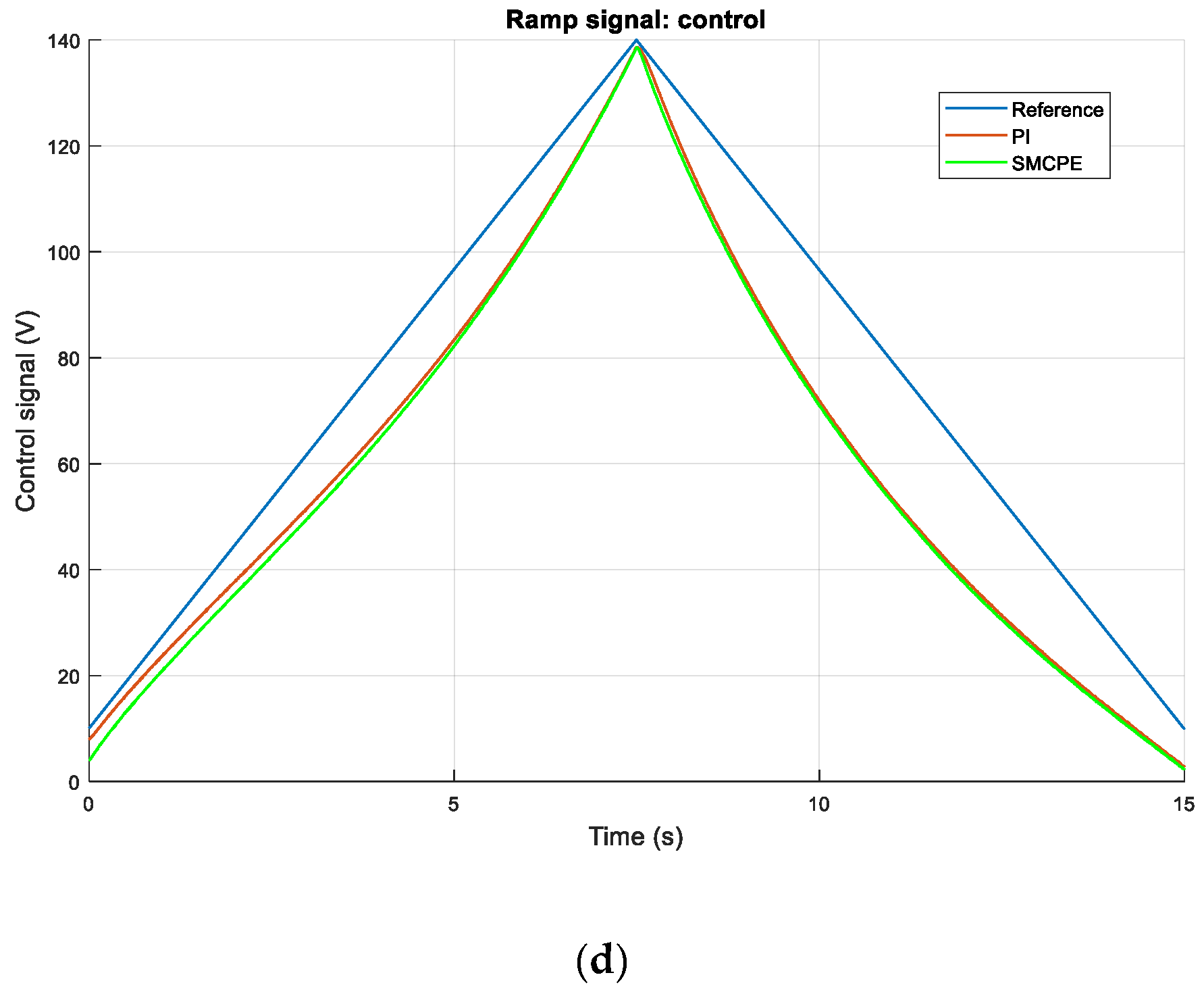
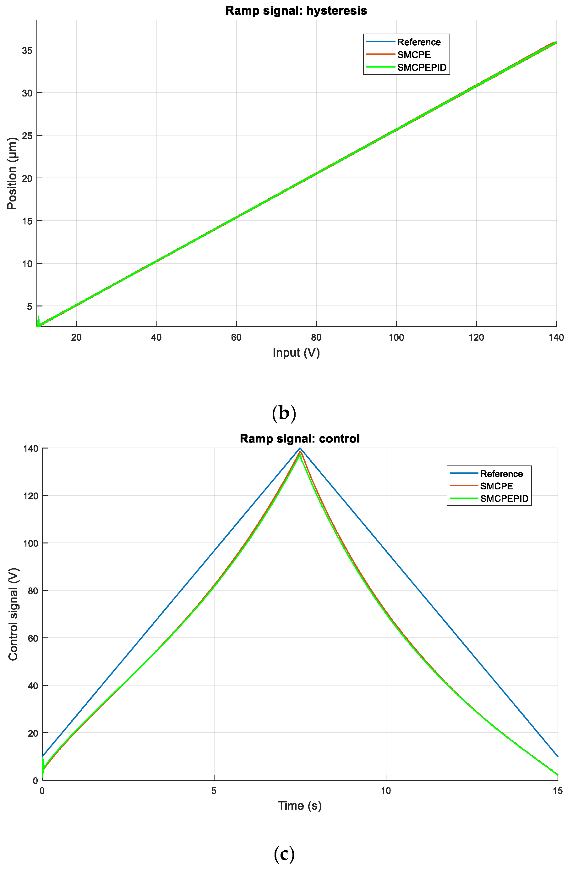
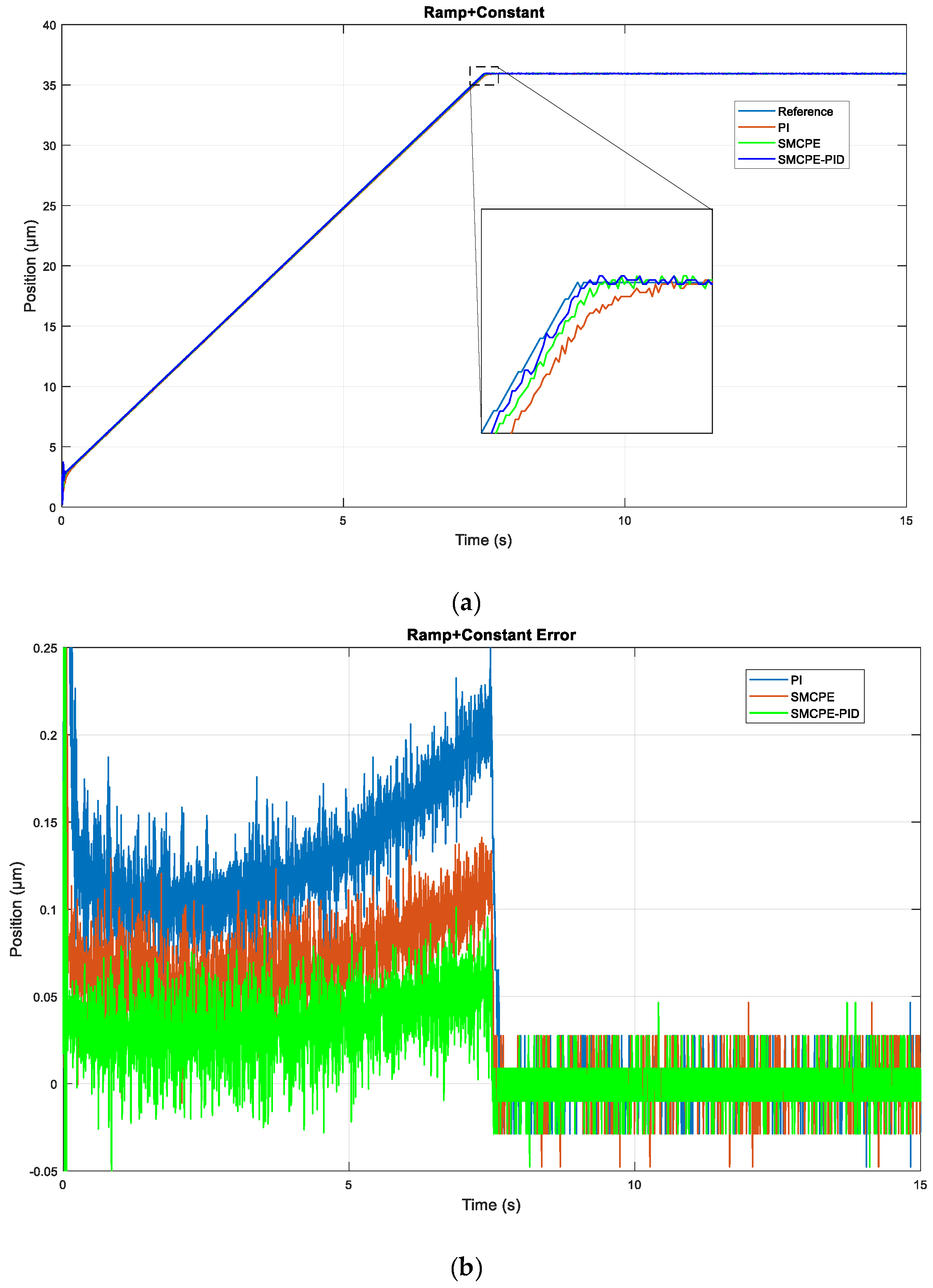
3.3. Ramp Signal Tracking

In addition, the capabilities of the PI and conventional SMCPE controllers to follow a ramp signal reference were compared. Then, the capabilities of the conventional SMCPE and PID sliding surface SMCPE controllers to follow a ramp signal reference were again compared. The reference signal used for the tests in this section was the same as the one described in Section 3.1.

In Figure 6, the performance of the system for the PI and SMCPE controllers is compared, when following a ramp signal. In Figure 6a, the reference ramp signal and displacement of the PEA are shown for both the PI and SMCPE controllers. In Figure 6b, the tracking errors obtained for both controllers are displayed. The error for the SMCPE controller was both smaller in its average and in its peak values, as well as having a similar form or pattern, thus being superior to the PI controller in every aspect. Following this, the IAE performance indicator shows that the SMCPE has a 55.5% smaller error than the PI (see

Table 3. Integral of the absolute magnitude of the error (IAE) performance indicators for ramp signal.

PI	1.9734 × 10−6
SMCPE	8.7837 × 10−7
SMCPE-PID	5.4097 × 10−7

). On a side note, an error difference smaller than 0.1 µm may not seem like much, but as PEAs are used for very high-precision applications, a small error difference like this can be significant. This is also applicable to the rest of the experimental results.

In Figure 6c, the resulting position–reference graph is displayed, showing that the hysteresis effect was completely eliminated. Finally, the control signals are displayed in Figure 6d. The control signal generated by the PI was a little bit more aggressive, which resulted in bigger maximum errors than for the SMCPE. Besides, there was no chattering at all, which shows that the chattering was eliminated by the controller, thanks to the saturation function (9) used.

As for the SMCPE and the SMCPE–PID, the comparison between them is displayed in Figure 7. As seen in Figure 7a, and similarly to what happens with the PI controller and the SMCPE, the average tracking error for the SMCPE–PID was smaller than for the SMCPE, as well as having a similar form or pattern, thus being superior to the SMCPE controller in every aspect. There is again a notable reduction in the error, as the IAE performance indicator shows a 38.4% reduction from the SMCPE to the SMCPE–PID. When comparing the performance of the PI to the SMCPE–PID, the IAE gives a 72.6% error reduction (see Table 3).

Besides, the resulting position–reference graph is displayed in Figure 7b, showing that in this case the hysteresis effect was also eliminated. Finally, the control signal was quite similar for both controllers, as displayed in Figure 7c. Again, the chattering effect has disappeared.

3.4. Constant Reference Tracking

In order to compare the performance of the PI, SMCPE, and SMCPE–PID under a constant reference, the following experimental validation was carried out. The control laws of both the SMCPE and SMCPE–PID controllers have a double derivative of the position reference (see (7, 11)). For this reason, a step signal could not be used as a reference for them, and a ramp signal followed by a constant reference was used instead. This signal went from 10 to 140 V with a 17.33 V/s speed and then stayed at 140 V for 7.5 s.

Results can be seen in Figure 8. As seen in Figure 8b, in the constant reference part, the response of the system was very similar for all the controllers. Meanwhile, in the ramp portion of the signal, the SMCPE–PID had the best performance, followed by the SMCPE, as analyzed in the section before. In other words, the constant reference tracking performance was mostly the same for the three controllers, but the SMCPE–PID had a better position tracking than both the SMCPE and PI.

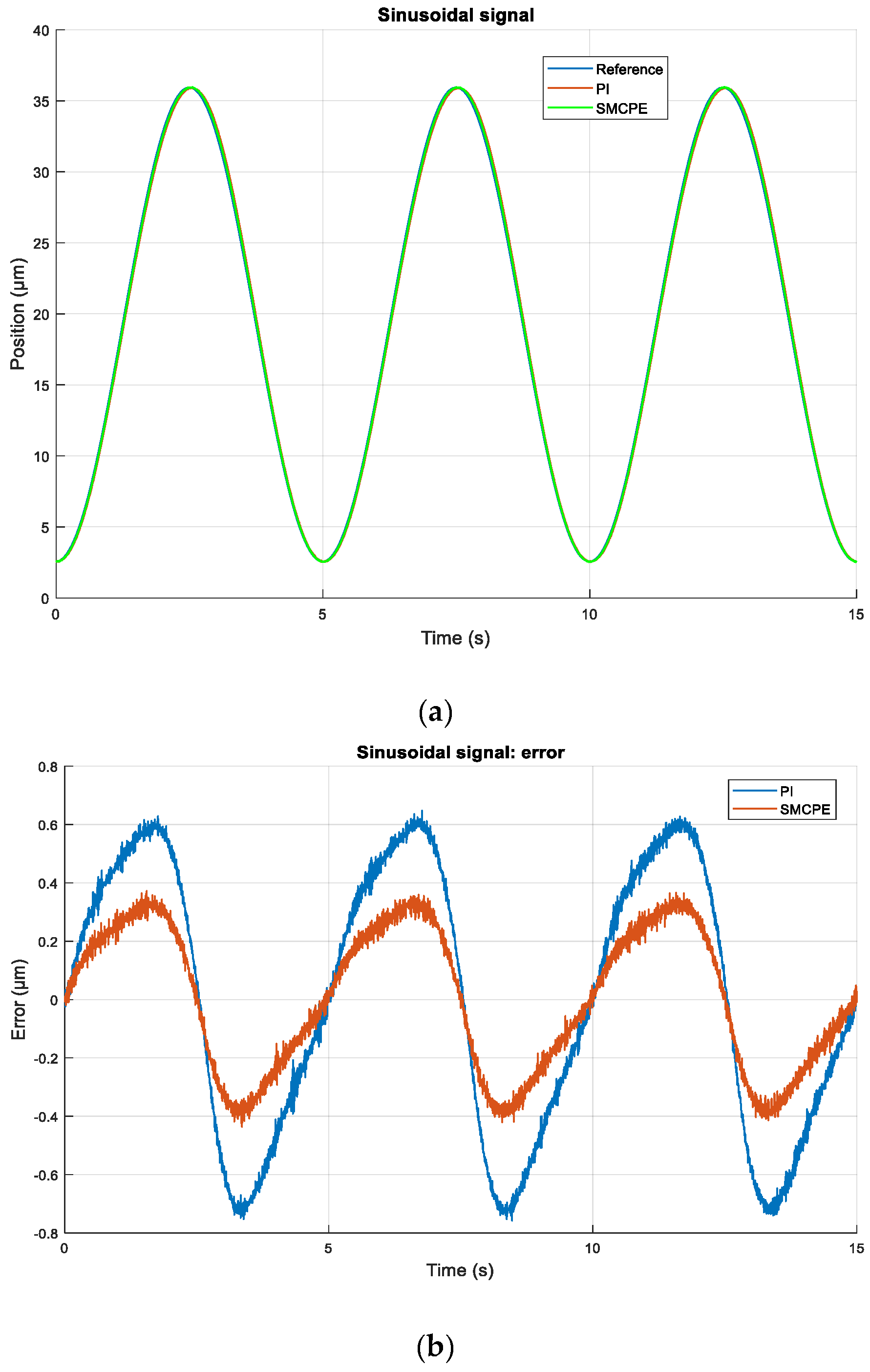
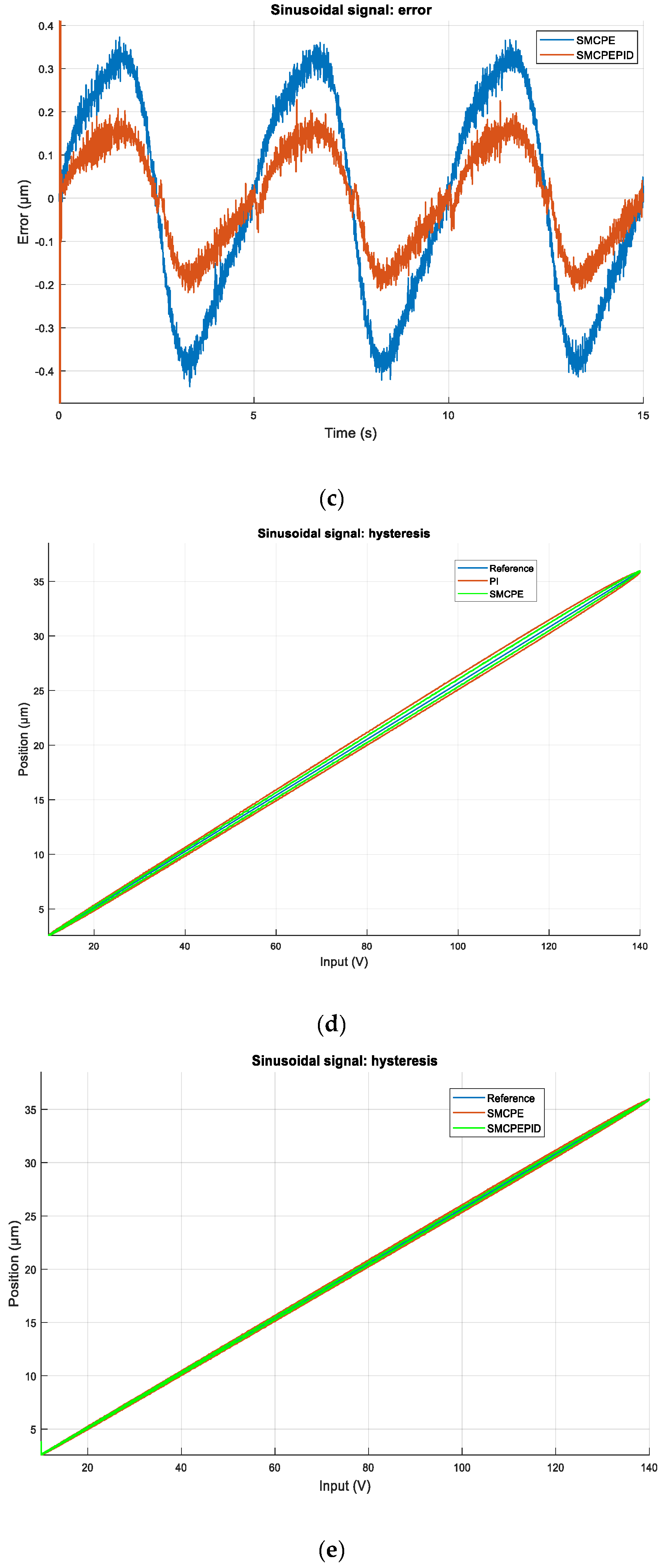
3.5. Sinusoidal Motion Tracking

The capabilities of the discussed controllers to track a sinusoidal signal were also examined. For this purpose, the tracking error and generated control signal were tracked and analyzed.

The reference signal used to study the sinusoidal motion tracking was a 0.2 Hz and 130 V peak-to-peak sinusoidal signal, with a 10 V offset. Thus, the position reference stayed in the 2.57–35.93 µm range.

In Figure 9, the experimental results of the PI, conventional SMCPE, and improved SMCPE–PID for sinusoidal motion tracking are displayed. First, in Figure 9a, the reference signal and PEA displacements for the PI and SMCPE controllers are presented. As in this graph the differences between the controllers are not that evident and its only purpose is to lay out the reference signal and the outputs, the tracking error is then displayed in Figure 9b. The same is done for the SMCPE–PID controller, comparing its results to the results of the SMCPE in Figure 9c. All the controllers had the same pattern regarding the reference signal: The tracking error was the biggest when the voltage change was zero, and the smallest when the voltage change was the maximum. From the three controllers, the SMCPE–PID had the smallest error, both in average and peak-to-peak. As for the IAE performance indicator, it shows that the SMCPE controller was 56.9% better than the PI, while the SMCPE–PID was 40.9% better than the SMCPE and 74.5% better than the PI (see

Table 4. IAE performance indicators for sinusoidal signal.

PI	6.0586 × 10−6
SMCPE	2.6139 × 10−6
SMCPE-PID	1.5441 × 10−6

).

The position–reference graph is also presented in Figure 9d,e, showing that the effect of the hysteresis was greatly decreased in both the SMCPE and the SMCPE–PID controllers, while it was still visible with the PI controller.

Finally, the control signals generated by the controllers, PI vs. SMCPE and SMCPE vs. SMCPE–PID, are displayed in Figure 9f,g, respectively. As with the control signal in the ramp signal tracking, the PI controller was a bit more aggressive than the others. Besides, there was no chattering to be seen.

4. Conclusions

In this paper, the experimental performance of a SMCPE and a SMCPE controller with a PID-type sliding surface were examined for motion tracking of a commercial PEA, comparing them to the more traditional PI controller. For the experimental validation, a control text bench was designed and constructed using a commercial piezoelectric actuator, a piezo driver, a strain gauge sensor, and a real-time embedded evaluation board myRIO. Moreover, some signal adaptation devices and some signal filters were also designed and implemented.

The importance of a good hysteresis model and usage of saturation function (9) for the correct performance of the SMCPE controllers was also demonstrated by means of some real experiments over a commercial piezoelectric actuator. As for the results, the ramp signal, constant reference, and sinusoidal motion tracking experiments showed that the proposed SMCPE–PID controller can improve the tracking performance, with the smallest peak-to-peak error and IAE performance indicator of the analyzed controllers, proving that it is a feasible control approach to deal with model imperfections and uncertainties for nonlinear systems.

With the proposed controllers, a submicron accuracy motion tracking has been achieved by the piezoelectric actuator. Since the implementation of the controller does not require any bounds on uncertainties and unknown parameters of the system, the proposed control can be used in the field of micro/nano-scale manipulation.

References

1. Abbott, J.J.; Nagy, Z.; Beyeler, F.; Nelson, B.J. Robotics in the small, part I: Microrobotics. IEEE Robot. Autom. Mag. 2007, 14, 92–103. [Google Scholar] [CrossRef]
2. Gu, G.Y.; Zhu, L.M.; Su, C.Y.; Ding, H.; Fatikow, S. Modeling and Control of Piezo-Actuated Nanopositioning Stages: A Survey. IEEE Trans. Autom. Sci. Eng. 2016, 13, 313–332. [Google Scholar] [CrossRef]
3. Devasia, S.; Eleftheriou, E.; Moheimani, S.O.R. A survey of control issues in nanopositioning. IEEE Trans. Control Syst. Technol. 2007, 15, 802–823. [Google Scholar] [CrossRef]
4. Li, Y.; Xu, Q. Adaptive Sliding Mode Control with Perturbation Estimation and PID Sliding Surface for Motion Tracking of a Piezo-Driven Micromanipulator. IEEE Trans. Control Syst. Technol. 2010, 18, 798–810. [Google Scholar] [CrossRef]
5. Rakotondrabe, M. Bouc-Wen Modeling and Inverse Multiplicative Structure to Compensate Hysteresis Nonlinearity in Piezoelectric Actuators. IEEE Trans. Autom. Sci. Eng. 2011, 8, 428–431. [Google Scholar] [CrossRef]
6. Gu, G.Y.; Zhu, L.M.; Su, C.Y. Modeling and Compensation of Asymmetric Hysteresis Nonlinearity for Piezoceramic Actuators with a Modified Prandtl-Ishlinskii Model. IEEE Trans. Ind. Electron. 2014, 61, 1583–1595. [Google Scholar] [CrossRef]
7. Lin, C.-J.; Yang, S.-R. Precise positioning of piezo-actuated stages using hysteresis-observer based control. Mechatronics 2006, 16, 417–426. [Google Scholar] [CrossRef] [Green Version]
8. Xu, H.G.; Ono, T.; Esashi, M. Precise motion control of a nanopositioning PZT microstage using integrated capacitive displacement sensors. J. Micromech. Microeng. 2006, 16, 2747–2754. [Google Scholar] [CrossRef]
9. Boukhnifer, M.; Ferreira, A. H∞ loop shaping bilateral controller for a two-fingered tele-micromanipulation system. IEEE Trans. Control Syst. Technol. 2007, 15, 891–905. [Google Scholar] [CrossRef]
10. Aphale, S.S.; Devasia, S.; Moheimani, S.O.R. High-bandwidth control of a piezoelectric nanopositioning stage in the presence of plant uncertainties. Nanotechnology 2008, 19, 125503. [Google Scholar] [CrossRef] [Green Version]
11. Liu, W.; Cheng, L.; Hou, Z.G.; Yu, J.; Tan, M. An Inversion-Free Predictive Controller for Piezoelectric Actuators Based on a Dynamic Linearized Neural Network Model. IEEE ASME Trans. Mechatron. 2016, 21, 214–226. [Google Scholar] [CrossRef]
12. Xu, R.; Zhou, M. A self-adaption compensation control for hysteresis nonlinearity in piezo-actuated stages based on Pi-sigma fuzzy neural network. Smart Mater. Struct. 2018, 27, 045002. [Google Scholar] [CrossRef] [Green Version]
13. Xu, Q. Digital Sliding-Mode Control of Piezoelectric Micropositioning System Based on Input–Output Model. IEEE Trans. Ind. Electron. 2014, 61, 5517–5526. [Google Scholar] [CrossRef]
14. Kuo, T.-C.; Huang, Y.-J.; Chang, S.-H. Sliding mode control with self-tuning law for uncertain nonlinear systems. ISA Trans. 2008, 47, 171–178. [Google Scholar] [CrossRef] [PubMed]
15. Xu, Q.S.; Li, Y.M. Micro-/Nanopositioning Using Model Predictive Output Integral Discrete Sliding Mode Control. IEEE Trans. Ind. Electron. 2012, 59, 1161–1170. [Google Scholar] [CrossRef]
16. Chen, X.K.; Hisayama, T. Adaptive Sliding-Mode Position Control for Piezo-Actuated Stage. IEEE Trans. Ind. Electron. 2008, 55, 3927–3934. [Google Scholar] [CrossRef]
17. Elmali, H.; Olgac, N. Sliding mode control with perturbation estimation (SMCPE): A new approach. Int. J. Control 1992, 56, 923–941. [Google Scholar] [CrossRef]
18. Bashash, S.; Jalili, N. Robust multiple frequency trajectory tracking control of piezoelectrically driven micro/nanopositioning systems. IEEE Trans. Control Syst. Technol. 2007, 15, 867–878. [Google Scholar] [CrossRef]
19. Ma, H.F.; Wu, J.H.; Xiong, Z.H. Discrete-Time Sliding-Mode Control with Improved Quasi-Sliding-Mode Domain. IEEE Trans. Ind. Electron. 2016, 63, 6292–6304. [Google Scholar] [CrossRef]
20. Slotine, J.J.E.; Spong, M.W. Robust robot control with bounded input torques. J. Robot. Syst. 1985, 2, 329–352. [Google Scholar] [CrossRef]
21. Stepanenko, Y.; Cao, Y.; Su, C.-Y. Variable structure control of robotic manipulator with PID sliding surfaces. Int. J. Robust Nonlinear Control 1998, 8, 79–90. [Google Scholar] [CrossRef]
22. Eker, I. Sliding mode control with PID sliding surface and experimental application to an electromechanical plant. ISA Trans. 2006, 45, 109–118. [Google Scholar] [CrossRef]
23. Low, T.S.; Guo, W. Modeling of a three-layer piezoelectric bimorphbeam with hysteresis. J. Microelectromech. Syst. 1995, 4, 230–237. [Google Scholar] [CrossRef]
24. Barambones, O.; Gonzalez de Durana, J.M.; Calvo, I. Adaptive Sliding Mode Control for a Double Fed Induction Generator Used in an Oscillating Water Column System. Energies 2018, 11, 2939. [Google Scholar] [CrossRef]
25. Utkin, V.I. Sliding mode control design principles and applications to electric drives. IEEE Trans. Ind. Electron. 1993, 40, 26–36. [Google Scholar] [CrossRef]
26. Slotine, J.J.E.; Li, W. Applied Nonlinear Control; Prentice-Hall: Englewood Cliffs, NJ, USA, 1991; ISBN 978-0130408907. [Google Scholar]
Figure 1. Experimental setup.
Energies 12 00943 g001
Figure 2. Nonlinear d curve.
Energies 12 00943 g002
Figure 3. Modelled hysteresis loop: (a) System Identification, and (b) System Verification.
Energies 12 00943 g003
Figure 4. Effect of hysteresis feedback in sliding mode control with estimation perturbation (SMCPE) controller: (a) Position, and (b) Position error.
Energies 12 00943 g004
Figure 5. Effect of saturation function in SMCPE controller.
Energies 12 00943 g005
Figure 6. PI vs. SMCPE performance comparison for ramp signal tracking: (a) Position, (b) Position error, (c) Position–reference, and (d) Control signal.
Energies 12 00943 g006aEnergies 12 00943 g006b
Figure 7. SMCPE vs. SMCPE–proportional–integral–derivative (PID) performance comparison for ramp signal tracking: (a) Error, (b) Position–reference, and (c) Control signal.
Energies 12 00943 g007aEnergies 12 00943 g007b
Figure 8. (a) Position and (b) Error.
Energies 12 00943 g008
Figure 9. (a) Position PI vs. SMCPE, (b) Position error PI vs. SMCPE, (c) Position error SMCPE vs. SMCPE–PID, (d) Position–reference PI vs. SMCPE, (e) Position–reference SMCPE vs. SMCPE–PID, (f) Control signal PI vs. SMCPE, and (g) Control signal SMCPE vs. SMCPE–PID.
Energies 12 00943 g009aEnergies 12 00943 g009bEnergies 12 00943 g009c