A Hybrid Neural Network Model for Power Demand Forecasting

Abstract

The problem of power demand forecasting for the effective planning and operation of smart grid, renewable energy and electricity market bidding systems is an open challenge. Numerous research efforts have been proposed for improving prediction performance in practical environments through statistical and artificial neural network approaches. Despite these efforts, power demand forecasting problems remain to be a grand challenge since existing methods are not sufficiently practical to be widely deployed due to their limited accuracy. To address this problem, we propose a hybrid power demand forecasting model, called (c, l)-Long Short-Term Memory (LSTM) + Convolution Neural Network (CNN). We consider the power demand as a key value, while we incorporate c different types of contextual information such as temperature, humidity and season as context values in order to preprocess datasets into bivariate sequences consisting of <Key, Context_{[1, c]}> pairs. These c bivariate sequences are then input into c LSTM networks with l layers to extract feature sets. Using these feature sets, a CNN layer outputs a predicted profile of power demand. To assess the applicability of the proposed hybrid method, we conduct extensive experiments using real-world datasets. The results of the experiments indicate that the proposed (c, l)-LSTM+CNN hybrid model performs with higher accuracy than previous approaches.

1. Introduction

Power demand forecasting is an important and challenging topic for the fields of smart grids, renewable energy and the electricity market bidding system. Power demand forecasting for the prevention of blackouts is becoming crucial globally as power consumption in businesses and homes rapidly increases. Optimum operation of the power system based upon accurate power demand forecasting is essential. Traditionally, governments and utilities have adopted a variety of methods to secure more power plants, including nuclear, hydropower, thermal power and renewable energy sources, to balance the demand and supply of electricity. Governments have also recently put considerable effort into increasing the efficiency of power systems by profiling the demand for power consumption and inhibiting the maximum demand during peak hours. The importance of power demand forecasting for predicting the profile of power demand is growing. Power demand forecasting facilitates the processing of estimating the required generation amount (power generation capability and reserve) in advance, and effectively controlling the demand (peak clipping and shifting).

We can classify power demand forecasting problems into three categories: short-term, medium-term, and long-term forecasting. Short-term forecasting is used to predict power demands over time periods of minutes, hours, days or weeks. Medium-term forecasting extends from months or one to two years, and long-term forecasting deals with predictions many years ahead.

Short-term power demand forecasting has been an active area of research. There are two main approaches: statistical methods and artificial neural networks. Statistical approaches include the Autoregressive Integrated Moving Average (ARIMA) [1], double seasonal Holt-Winters exponential smoothing [2] and PCA-based Linear Regression [3]. Recently, artificial neural network-based approaches have received considerable attention in power demand forecasting. In an artificial neural network model, the model architecture varies depending upon both the period to be predicted and the data required to make the prediction. Broadly speaking, there are two type of sequences: univariate or multivariate. Models using univariate datasets tend to be simple, small in size and quick to train, but they have low accuracy, while models based on multivariate datasets are slower and more computationally intensive in practice. To address these problems, we first preprocess a given dataset into multi-bivariate sequences to effectively learn the features that can be extracted from individual context information. Then, we exploit a novel hybrid network model to accurately predict an n-day profile of power demand. Specifically, the proposed hybrid network consists of multi-LSTM layers and a CNN layer. In the multi-LSTM layers, each layer extracts features from each input, comprised of a bivariate (power and contextual information) sequence, and feeds these feature sets to a CNN layer to obtain an n-day profile. The proposed hybrid model is aimed at general forecasting problems with all short-term level of temporal granularities (minutes, hours, days etc.). The rationale of the proposed hybrid model design is to combine the efficiency of multi-LSTM in extracting features from various context information with the ensemble potential of CNN by introducing a bivariate-based context learning approach.

The rest of the paper is organized as follows: in Section 2, we introduce related researches on power demand forecasting using artificial neural networks and hybrid models. Section 3 first describes the pre-processing of the datasets and then depicts our hybrid network model. Section 4 describes the experimental methods and results. Lastly, Section 5 concludes the paper.

2. Related Work

2.1. Power Demand Forecasting Using Deep Learning

Most of the techniques used to predict power demand have included Recurrent Neural Network (RNN)-based LSTMs, which have used on time series data and natural language processing [4,5]. In particular, CNNs have produced high classification and recognition performance in the field computer vision and pattern recognition [6,7,8] and have also been demonstrated to be effective in various fields involving time series data such as language data, human behavior pattern data, energy load data etc. [9,10,11].

An ensemble deep learning method using several deep learning networks was described in [9]. In this paper, based on the observation that the output value changes when the number of epochs is changed, output values were obtained by using different epochs for each Deep Belief Network (DBN) over several DBNs. The authors then constructed an ensemble deep learning network using the output from a Support Vector Regression (SVR) as input and showed 4% and 15% better performance in predicting power demand than was obtained using SVR and DBN, respectively. In [10,11], time series data were processed using a multi-channel Deep CNN model which learns features from an individual univariate time series in each channel, and combines information from all channels to produce a feature representation at the final layer. This method was also applied to human behavior pattern data and ECG (electrocardiogram) data.

Most of the studies using artificial neural networks for power demand forecasting have used data from residential buildings, commercial or office buildings. Experiments on solar powered buildings have also been conducted [12]. These experiments used power demand data from business days, non-business days, and seasonal data. The model was optimized by adjusting the numbers of features and neurons. A study using two types of artificial neural network models was described in [13]. One model used a pre-trained Restricted Boltzmann machine (RBM), the other used a Rectified Linear Unit (ReLU) without pre-training. These models obtained better results in predicting the future 24 h than ARIMA or Shallow Neural Network (SNN). For small power systems with non-linear and non-critical characteristics, [14] used an LSTM model to predict power demand. The amount of power used in residential areas was divided into smaller groups, down to individual households. A study using the LSTM model to forecast the power demand for each household was conducted [15]. The authors forecasted the amount of power needed in the future based upon the current amount of power produced in a solar power plant. The LSTM, DBN, and Auto-LSTM were used in the experiment, and the Auto-LSTM had the best performance. Reference [16] proposed the Augmented LSTM (ALSTM) network method, which enhances the Auto-LSTM network method used in [17] by combining the AutoEncoder and LSTM. A study was carried out on forecasting power demand after 60 h by constructing the encoder and decoder using a Sequence to Sequence (S2S) structure-based on an LSTM. This work reported in [18] (Figure 1). This study mapped the date of the next day, not the current date, to power values. When power values and dates of the same day are used as inputs, the predicted values of the same day simply follow the pattern of the previous power values.

In order to improve the accuracy of the estimate of power demand for individual households, [19] proposed Pooling-based Deep-RNN (PDRNN). This study used the power data from the target household as well as those from neighboring power areas. The root mean square error (RMSE) of PDRNN was much lower: 19.5%, 13.1% and 6.5% compared to results from the ARIMA, SVR and classical deep RNNs.

To predict the power demand for individual buildings, the network in [20] was constructed using only a CNN, and was evaluated with only changing parameters. The data model used in [20] differs from existing methods in that only the power data is input to the first CNN layer, and the final fully connected layer incorporates information such as date and temperature, to predict power demand. In order to evaluate its performance, the proposed network, a Support Vector machine (SVM) and RBM were compared [20]. Experimental results showed better performance than previous methods, but the network model in [20] was not better than the method described in [18]. The use of CNN-based bagging techniques for smart grid load forecasting was reported in [21]. In reference [22], the USA District public consumption dataset and load dataset for 2016 provided by the Electric Reliability Council of Texas were processed using multiple CNNs to forecast power demand.

In the area of Natural Language Processing (NLP), RNNs, which are excellent for time series data processing, are primarily used. In order to improve an RNN’s performance, it is necessary to carefully select useful contextual information. Reference [23] conducted a study to predict where users should move next by selecting time and space as the contextual information, in order to achieve better results than traditional RNN models. Similarly, reference [24] introduced an RNN which is dependent on contextual information. In this study, when using input words to predict the next word, a feature layer with context information about the sentence topic was added.

2.2. Approaches Based on a Hybrid Network Model

One of the hybrid network structures for power demand forecasting is the CLDNN (a unified architecture of CNN, LSTM, and DNN) structure proposed in [25]. In this model as shown in Figure 2, LSTM layers were stacked on top of a CNN to create a hybrid network. This model was proposed for natural language processing, and the results on the power demand prediction problem showed limited prediction accuracy.

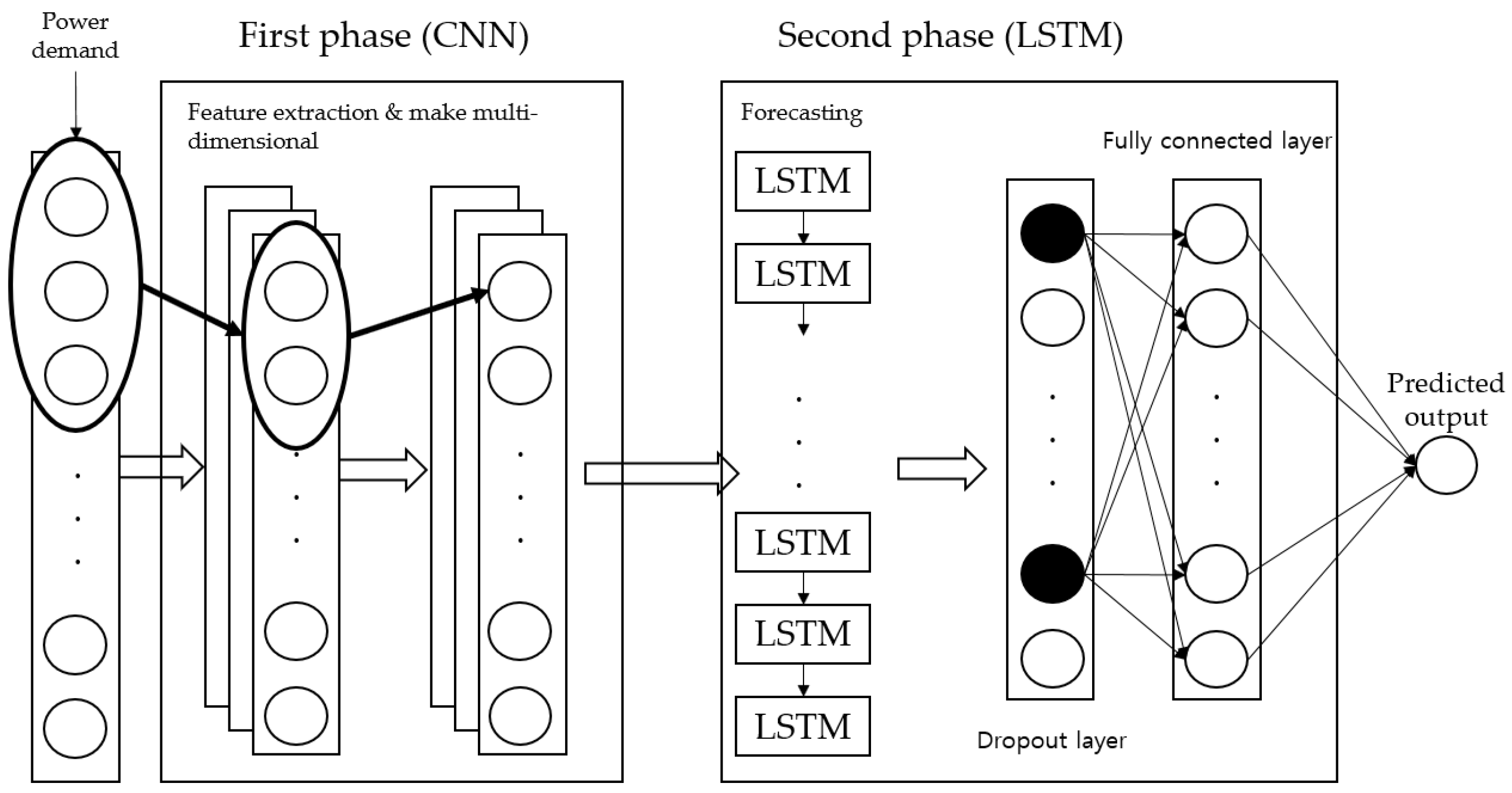
In reference [26], CNNs and LSTMs were used together to construct a framework consisting of two phases, to estimate power demand (Figure 3). The first function of the CNN layer is to extract the features of the power data, and the second function is to transform the one-dimensional power data into a multidimensional dataset by using the output of the CNN as input to the second phase, LSTM. The results are output through the dropout [27] layer. In reference [26], multi-step forecasting was performed, unlike traditional power demand forecasting methods based on a one-step forecasting.

Hybrid network studies for predicting power demand were also reported in [28,29]. In reference [28], the authors transformed a dataset into 2D images and used those images as inputs to a CNN-RNN model. The accuracy of the CNN-RNN was 10% and 26% higher than that of an LSTM and an ANN [30], respectively. Another study with a CNN-LSTM based hybrid framework was proposed in [29]. In this study, CNN and LSTM were arranged horizontally and the characteristics of the input data were extracted separately. After feature extraction by the CNN and the LSTM, the outputs of the two networks were concatenated in the merge layer of a feature-fusion layer.

In this paper, we propose the (c, l)-LSTM+CNN hybrid prediction model. As discussed in Section 3.2, we place multi-LSTM networks at the front to extract feature sets. Then, we create an ensemble by adding a CNN layer after the LSTMs in order to produce the final output.

3. Data Processing and Deep Learning Models

3.1. Data Processing

3.1.1. Vertical Partitioning and <Key, Context_{[1, c]}> Pairing

In power demand forecasting, there are two general types of sequences: univariate or multivariate. Models based on univariate datasets simply use the power demand values. The model size is therefore relatively small, and training time is fast. However, these models have the disadvantage that the error rate is inapplicable because context information is excluded. Models based on multivariate datasets include context information in addition to the power demand values. These models generally show better performance because of the addition of the context information. The model in [18] used this type of data, and showed better performance than other models.

Power demand forecasting can be influenced by many factors that can change patterns of load consumption. In this paper, we consider the power value as a Key value, and the other context domains as c Context information. We vertically divide a given dataset into sets of <Key, Context_{[1, c]}> pairs such as <power, temperature> or <power, day>. We create five bivariate sequences using five context domains: temperature, humidity, holiday status, day of the week, and season.

Table 1. Data notation.

Power	Key
Context Information	Context
Number of Domains	c
Data Pair Set	<Key, Context[1, c]>
Number of LSTM Layers	l

summarizes the data notation used in this paper. This pairing scheme enables the proposed model to be scalable with increasing numbers of context domains by simply adding additional <Key, Context> pairs.

3.1.2. Overlapped Window and Dataset

In order to predict the power demand for seven future days, we use the previous 14 days’ worth of information as training data. Specifically, we use a 14-day overlapped window with a one-day stride, as shown in Figure 4. The red box in Figure 4 is the first 14-day window used for training, and the blue box is the second 14-day window, to be learnt after sliding the window by one day.

In this paper, we use Korea’s daily power demand dataset [31] provided by the Korea Power Exchange. This dataset is a set of daily power demand values for each day from 1 January 2006 to 20 May 2017. Specifically, it consists of 4158 power demand values. As mentioned in Section 3.1.1, these power demand values are paired with five context domains: temperature, humidity, holiday status, day of the week, and season, resulting in five bivariate sequences in the form of <Key, Context_{[1, c]}>.

To further investigate the performance behavior, we classify the dataset into six categories. The reason for dividing the dataset into the categories shown in

Table 2. Training sets used in the experiments.

Holidays Status	Dataset Type	Notation	Size of Training Set	Window Size
With holidays	All-day dataset	d1	24,948	14
	Seasonal dataset	d2	5105	5
	Dataset by day	d3	2950	14
Without holidays	Weekday dataset	d4	14,225	10
	Seasonal dataset	d5	2680~2780	5
	Dataset by day	d6	2240~2280	10

is that the power demand amount during the weekend is different from that during the weekdays. As shown in Figure 5a,b, seasonal power demand is different, and overall it is apparent that weekend power demand is less than during weekdays. Therefore, when constructing our training datasets, we first divide the dataset by the presence or absence of holidays. Then, as shown in Table 2, six training datasets are constructed by classifying the dataset using all days of the week, seasonal dataset, and dataset by day. The data size of d₁ is 24,948 because it consists of 4158 daily power values and five context values for each day, while the data size d₂ is 5105 because it consists of 1021 daily power values per season and four context values (excluding season) for each day. The reason that the data sizes of d₅ and d₆ vary 2680~2780 and 2240~2280, respectively is because the number of holidays included in the weekday is different.

3.2. (c, l)-LSTM+CNN Hybrid Forecasting Model

Several studies have shown that LSTMs show good performance when learning time series data [14,15,16,17,18]. In reference [32], three different network types—CNN, LSTM, and DNN—were used to improve speech recognition performance. After training the three networks separately, three outputs were generated, and a combination layer was added. In reference [25], it was suggested that the design of combining the three separate networks results in better performance than that of any of the networks individually. With these observations in mind, we propose a hybrid deep learning neural network framework combining LSTM neural network with CNN to deal with the power demand forecasting problem. This hybrid network consists of c LSTM networks with l layers, followed by a CNN. Unlike the data preprocessing method used in the previous studies, the proposed hybrid model extracts the features of a dataset using an LSTM neural network in front stage. As mentioned in the previous section, the dataset is preprocessed into bivariate sequences in the form of <Key, Context_{[1, c]}> pairs. Each bivariate sequence is used as the input to an LSTM network with l layers. The LSTM network is composed of l layers, as shown in Figure 6, and acts as a node in the entire network structure, as shown in Figure 7.

We use 20 units of each LSTM and train each with data from the past 14 days. The feature set extracted from each LSTM network is a 14 × 20 matrix. We then integrate these feature sets to produce the input to the CNN. Specifically, we combine the feature sets of the c (=5) LSTM networks into one 14 × 20 matrix using element-wise multiplication. This matrix is passed to the input of the CNN layer to get the power demand forecast for the next seven days.

In this study, we use multi two-hidden-layer LSTMs and a two-hidden-layer CNN. After the CNN layer, we apply max-pooling (=2) once. There are 495 neurons in the proposed model structure and 60,363 parameters. In our proposed hybrid model, we use the Grid Search function provided by SciKit-learn [33] to optimize the entire model. If we specify a range of hyperparameters, this function learns by changing each parameter value within the given range and returns the value at which the optimum result is obtained. Specifically, when we specify a range of the value of hyperparameters, we take into account the data range and data size of our datasets, and as a result, we use 64 filters, a kernel size of three for each CNN layer as described in

Table 3. Optimization of hyperparameters.

Filter Size	1, 8, 16, 32, 64, 128
Kernel Size	1, 3, 5
Batch Size	7, 14, 21, 28, 35, 42
Epoch	10, 30, 50, 70, 80, 100, 120, 140
Optimizer	SGD, RMSprop, Adagrad, Adadelta, Adam, Adamax, Nadam

. The loss value, which is the difference between the predicted output $\widehat{y}$ and the expected output $y$, is computed as the mean squared error. The optimization process uses the gradient descent optimization algorithm called the Adam optimizer [34], which is commonly used for weight optimization of deep neural networks. The activation function applied to the network for each layer is the ReLU.

4. Experiments and Results

In this section, we assess the efficiency and effectiveness of the proposed (c, l)-LSTM+CNN hybrid model by comparing it against three widely-used models, ARIMA, (c, l)-LSTM and S2S LSTM. Note that (c, l)-LSTM is a model that does not include the CNN layer used in our proposed model. In this paper, two metrics are used to evaluate the forecasting accuracy of the model. One is the mean absolute percentage error (MAPE) (Equation (1)), and the other is the relative root-mean-square error (RRMSE) (Equation (2)) called the power consumption prediction error rate. Smaller values of the error metrics indicate higher forecasting accuracy:

$$\mathrm{MAPE}=\frac{{{\displaystyle \sum }}_{i=1}^N\left|\frac{\widehat{y_i}-y_i}{y_i}\right|\times 100}{N}$$

(1)

$$\mathrm{RRMSE}=\sqrt{\frac{{{\displaystyle \sum }}_{i=1}^N{\left(y_i-\widehat{y_i}\right)}^2}{{{\displaystyle \sum }}_{i=1}^N{y}_i{}^2}\times 100}$$

(2)

where $y_i$ is an actual test value; ${\widehat{y}}_i$ is the forecasting result of $y_i$; and N is the total number of testing samples.

4.1. Experiment Environment and Determination of the Number of Layers l

The proposed (c, l)-LSTM+CNN hybrid model is implemented using Python 3.5.2 (64-bit) with PyCharm Community Edition 2016.3.2. The hardware configuration includes an Intel Core i7-5820k CPU@3.3GHz, 32G RAM and a NVIDIA GeForce GTX780 graphics card. The proposed hybrid model is built using Tensorflow [35] with Keras [36] version 2.1.5 as the front-end interface.

Different values for the number of layers parameter l, may lead to different accuracies, and this parameter thus may have a non-trivial impact on the overall performance of the proposed hybrid model. In this section, we focus on determining a value for l that obtains the minimum prediction error. We conduct a set of experiments to determine l in LSTM networks. The dataset used for these experiments is the all-day dataset d₁. We conduct four sets of experiments varying l from 1 to 4 (

Table 4. Errors by l values for the (c, l)-LSTM+CNN hybrid forecasting model with d₁.

Number of Layers l	MAPE (%)	RRMSE (%)
l = 1	3.60	4.47
l = 2	1.45	1.83
l = 3	1.85	2.08
l = 4	2.02	2.36

and Figure 8). Since the results of these experiments show that the highest accuracy is achieved at l = 2, we set the number of layers l in each LSTM network to 2.

4.2. Case 1: With Holidays

We first present the results of experiments using the datasets of d₁, d₂ and d₃, which include holidays. The dataset d₁ includes all days of the week, while the datasets d₂, d₃ are classified by season and by day of the week, respectively. As mentioned in Section 3.1.2, we use a daily power demand sequence from 1 January 2006 to 20 May 2017 as training data. In addition, we use five types of context information: average temperature, humidity, holiday status, day of the week, and seasons. Most studies on forecasting power demand provide only hourly or daily predictions [37,38,39]. To address this issue, we choose a next 7-day profile as a target profile from 21 May 2017 to 27 May 2017 for performance evaluation.

Figure 9, Figure 10 and Figure 11 show the prediction results for each dataset, i.e., d₁, d₃ and d₂, respectively. As shown in Figure 9, Figure 10 and Figure 11, the proposed (c, l)-LSTM+CNN hybrid model shows lower forecasting error and consequently higher forecasting accuracy compared with the ARIMA model, (c, l)-LSTM and S2S LSTM for all datasets. The proposed hybrid model shows the highest accuracy when trained on the dataset d₃ (Figure 10).

In order to further investigate the characteristics of the datasets, we present the results of power demand forecasts for each model in Figure 12a–d. As shown in Figure 12a, ARIMA, which uses only power values for training, shows a similar pattern through all datasets, although the best result is achieved with d₃. Figure 12b shows the (c, l)-LSTM closely reflects the actual power values pattern when using d₂-spring, although the experiments using d₁ and d₃ are not as successful. Although the S2S LSTM shows better results than ARIMA and the (c, l)-LSTM when using d₃ in Figure 12c, it does not outperform our proposed (c, l)-LSTM+CNN hybrid model. As shown in Figure 12d, the proposed (c, l)-LSTM+CNN hybrid model most accurately predicts the actual values when compared with other models.

The average forecasting errors of models trained on datasets d₁, d₂ and d₃ are summarized in

Table 5. Errors for d₁, d₂ and d₃.

Dataset	Season	MAPE (%)				RRMSE (%)
		ARIMA	(c, l)-LSTM	S2S LSTM	Proposed Model	ARIMA	(c, l)-LSTM	S2S LSTM	Proposed Model
d1	-	4.78	3.42	2.66	1.45	5.70	3.93	2.86	1.83
d2	Spring	4.07	2.62	3.09	2.30	4.87	2.98	3.83	2.54
	Summer	4.32	3.13	3.51	2.35	5.09	3.78	3.64	2.57
	Autumn	5.45	2.67	2.88	2.09	6.52	3.15	3.77	2.75
	Winter	5.17	3.20	3.96	2.77	6.04	3.69	4.52	3.19
d3	-	3.17	3.35	1.64	0.81	3.85	3.84	2.02	1.17

. Our proposed (c, l)-LSTM+CNN hybrid model produces better results when using d₃ than when using d₁ or d₂. Also, the proposed hybrid model shows better forecasting accuracy than the ARIMA, (c, l)-LSTM and S2S LSTM models. The prediction errors (MAPE) of the proposed model trained on d₁ are 70%, 58% and 45% lower than ARIMA, (c, l)-LSTM and S2S LSTM, respectively. In addition, the MAPE of the proposed model trained on d₂ are up to 4% lower than those of ARIMA, (c, l)-LSTM and S2S LSTM. In particular, the (c, l)-LSTM+CNN trained on d₃ shows the best forecasting accuracy by, on average, 0.81% and 1.17% for MAPE and RRMSE, respectively. The MAPE of our model is much lower by 74%, 76% and 51% compared to the ARIMA, (c, l)-LSTM and S2S LSTM, respectively.

4.3. Case 2: Without Holidays

As mentioned in Section 3.1.2, the pattern of power demand on weekends and holidays differs from that on weekdays, making it difficult for models to learn the underlying patterns, if trained on all of the data. To further investigate this fact, we divide the dataset without holidays into three categories, d₄, d₅ and d₆, as shown in Table 2.

Figure 13, Figure 14 and Figure 15 present the performance of each model using the datasets d₄, d₆ and d₅, respectively. From these figures, we observe that the datasets without holidays (d₄, d₅ and d₆) are more effective for training models than the datasets with holidays (d₁, d₂ and d₃). In particular, as shown in Figure 14, the proposed (c, l)-LSTM+CNN hybrid model shows the best forecasting accuracy when using the dataset d₆.

To further analyze the forecasting performance of each model, we present the forecasting result for each model in Figure 16a–d. As can be seen from Figure 16a, ARIMA trained on d₄ and d₅ shows similar patterns, but shows a different pattern when trained on d₆. Figure 16b,c show the results of the (c, l)-LSTM and S2S LSTM, respectively.

When compared with ARIMA, we can see that the results of these two models are closer to the actual values than ARIMA. In Figure 16d, it is clear that the proposed (c, l)-LSTM+CNN hybrid model produces results closer to the actual power value pattern for most of the datasets than do the other models. In particular, the proposed hybrid model shows the best results when using d₆.

The average errors of models using d₄, d₅ and d₆ are described in

Table 6. Errors for d₄, d₅ and d₆.

Dataset	Season	MAPE (%)				RRMSE (%)
		ARIMA	(c, l)-LSTM	S2S LSTM	Proposed Model	ARIMA	(c, l)-LSTM	S2S LSTM	Proposed Model
d4	-	2.20	2.53	1.20	1.26	2.24	2.59	1.80	2.04
d5	Spring	2.21	1.59	1.38	1.00	2.25	1.91	2.19	1.15
	Summer	2.08	2.99	1.27	2.08	2.13	3.12	1.43	2.27
	Autumn	2.37	1.76	3.10	1.27	2.43	1.92	3.54	1.64
	Winter	2.18	2.57	2.28	2.70	2.23	2.92	2.32	2.99
d6	-	3.61	2.34	0.84	0.82	3.85	2.44	1.40	0.90

. When compared with Table 5 in Section 4.2, we observe that the overall accuracy is improving. As can be seen in Table 6, the (c, l)-LSTM+CNN hybrid forecasting model trained on d₆ has better accuracy than any of the other models. Specifically, the proposed (c, l)-LSTM+CNN hybrid model shows the best accuracy on average by 0.82% for MAPE and 0.90% for RRMSE. On the other hand, the RRMSEs of ARIMA, (c, l)-LSTM and S2S LSTM are 3.85%, 2.44%, and 1.40% on average, respectively. The proposed hybrid model shows 77%, 63% and 36% lower prediction error (RRMSE) than ARIMA, (c, l)-LSTM and S2S LSTM, respectively.

4.4. Forecasting an n-Day Profile

As discussed in Section 1, the proposed (c, l)-LSTM+CNN hybrid model can be applied to general forecasting problems with any temporal granularity. To assess the efficacy of our proposed model for predicting over longer time periods, we present the results of predicting a 21-day profile as shown in Figure 17. The MAPE and RRMSE of S2S LSTM is 2.99% and 3.59%, respectively, while the proposed (c, l)-LSTM+CNN hybrid model is able to predict a 21-day profile with forecasting accuracy of 0.91% and 1.13% in MAPE and RRMSE, respectively. These results indicate that the proposed (c, l)-LSTM+CNN hybrid model scales well with time.

5. Conclusions

In this paper, we propose a hybrid model for forecasting power demand for an n-day profile by combining the benefits of LSTMs and CNNs. Unlike previous studies using univariate or multivariate sequences, we preprocess a dataset by pairing a power demand value (Key) with a context value (Context_c), resulting in <Key, Context_{[1, c]}> bivariate sequences to efficiently reflect important context information to be used when training hybrid neural networks. We propose a (c, l)-LSTM+CNN hybrid forecasting model consisting of (c, l)-LSTM for extracting features from each bivariate sequence, and a CNN for ensembling these feature sets to derive a predicted profile of power demand.

Extensive experiments are conducted by dividing the dataset into two groups: with holidays and without holidays. Each group of datasets is divided into an all-days dataset, a seasonal dataset and a dataset by day of the week. We compare our proposed hybrid network with existing methods: ARIMA, (c, l)-LSTM and S2S LSTM. In particular, when we use the dataset (d₆) by day of the week without holidays, the proposed (c, l)-LSTM+CNN hybrid model shows the best accuracy on average by 0.82% and 0.90% in terms of MAPE and RRMSE. Specifically, the proposed hybrid model shows 77%, 63% and 36% lower prediction error (RRMSE) than ARIMA, (c, l)-LSTM and S2S LSTM, respectively.

Since the proposed hybrid model can be applied to general forecasting problems at all short-term levels of temporal granularity, it can be extended in various directions. In particular, we expect that the proposed hybrid model can also be applied to other types of time series such as indoor human behavioral patterns, 12-lead ECG (electrocardiogram) etc. As another example, the proposed hybrid model can be applied to the 15-minutely or hourly prediction of photovoltaics (PV) generation by considering various context information such as temperature, cloudiness, air quality index (PM2.5, PM10, O₃, NO₂, SO₂, CO).

In addition, the importance of forecasting electricity demand in factories and houses at small-scale units with short temporal granularity is recently emerging. To deal with this issue, we are currently collecting relevant data, and plan to augment our proposed hybrid model with small-scale electric power demand forecast ability to support prosumers. In future work, we plan to extend our hybrid model to produce medium-term forecasts for horizons of lengths ranging from a few months to one to two years.

References

1. Yuan, C.; Liu, S.; Fang, Z. Comparison of China’s primary energy consumption forecasting by using ARIMA (the autoregressive integrated moving average) model and GM (1, 1) model. Energy 2016, 100, 384–390. [Google Scholar] [CrossRef]
2. Taylor, J.W. Short-term electricity demand forecasting using double seasonal exponential smoothing. J. Oper. Res. Soc. 2003, 54, 799–805. [Google Scholar] [CrossRef] [Green Version]
3. Bair, E.; Hastie, T.; Paul, D.; Tibshirani, R. Prediction by supervised principal components. J. Am. Stat. Assoc. 2006, 101, 119–137. [Google Scholar] [CrossRef]
4. Wen, T.H.; Gasic, M.; Mrksic, N.; Su, P.H.; Vandyke, D.; Young, S. Semantically conditioned LSTM-based natural language generation for spoken dialogue systems. arXiv, 2015; arXiv:1508.01745. [Google Scholar]
5. Sundermeyer, M.; Ney, H.; Schlüter, R. From feedforward to recurrent LSTM neural networks for language modeling. IEEE/ACM Trans. Audio Speech Lang. Process. 2015, 23, 517–529. [Google Scholar] [CrossRef]
6. Krizhevsky, A.; Sutskever, I.; Hinton, G.E. Imagenet classification with deep convolutional neural networks. Adv. Neural Inf. Process. Syst. 2012, 25, 1106–1114. [Google Scholar] [CrossRef]
7. Szegedy, C.; Liu, W.; Jia, Y.; Sermanet, P.; Reed, S.; Anguelov, D.; Erhan, D.; Vanhoucke, V.; Rabinovich, A. Going deeper with convolutions. In Proceedings of the IEEE Conference on Computer Vision and Pattern Recognition, Boston, MA, USA, 7–12 June 2015. [Google Scholar]
8. Chen, L.C.; Papandreou, G.; Kokkinos, I.; Murphy, K.; Yuille, A.L. Deeplab: Semantic image segmentation with deep convolutional nets, Atrous convolution, and Fully connected CRFs. IEEE Trans. Pattern Anal. Mach. Intell. 2018, 40, 834–848. [Google Scholar] [CrossRef] [PubMed]
9. Qiu, X.; Zhang, L.; Ren, Y.; Suganthan, P.N.; Amaratunga, G. Ensemble deep learning for regression and time series forecasting. In Proceedings of the 2014 IEEE Symposium on Computational Intelligence in Ensemble Learning (CIEL), Orlando, FL, USA, 9–12 December 2014. [Google Scholar]
10. Zheng, Y.; Liu, Q.; Chen, E.; Ge, Y.; Zhao, J.L. Time series classification using multi-channels deep convolutional neural networks. In International Conference on Web-Age Information Management; Springer: Cham, Switzerland, 2014. [Google Scholar]
11. Yang, J.; Nguyen, M.N.; San, P.P.; Li, X.L.; Krishnaswamy, S. Deep Convolutional Neural Networks on Multichannel Time Series for Human Activity Recognition. In Proceedings of the Twenty-Fourth International Joint Conference on Artificial Intelligence (IJCAI 2015), Buenos Aires, Argentina, 25–31 July 2015. [Google Scholar]
12. Khosravani, H.; Castilla, M.; Berenguel, M.; Ruano, A.; Ferreira, P. A comparison of energy consumption prediction models based on neural networks of a bioclimatic building. Energies 2016, 9, 57. [Google Scholar] [CrossRef]
13. Ryu, S.; Noh, J.; Kim, H. Deep neural network based demand side short term load forecasting. Energies 2016, 10, 3. [Google Scholar] [CrossRef]
14. Zheng, J.; Xu, C.; Zhang, Z.; Li, X. Electric load forecasting in smart grids using long-short-term-memory based recurrent neural network. In Proceedings of the 2017 51st Annual Conference on Information Sciences and Systems (CISS), Baltimore, MD, USA, 22–24 March 2017. [Google Scholar]
15. Kong, W.; Dong, Z.Y.; Jia, Y.; Hill, D.J.; Xu, Y.; Zhang, Y. Short-term residential load forecasting based on LSTM recurrent neural network. IEEE Trans. Smart Grid 2019, 10, 841–851. [Google Scholar] [CrossRef]
16. Hsu, D. Time Series Forecasting Based on Augmented Long Short-Term Memory. arXiv, 2017; arXiv:1707.00666. [Google Scholar]
17. Gensler, A.; Henze, J.; Sick, B.; Raabe, N. Deep Learning for solar power forecasting—An approach using AutoEncoder and LSTM Neural Networks. In Proceedings of the 2016 IEEE International Conference on Systems, Man, and Cybernetics (SMC), Budapest, Hungary, 9–12 October 2016. [Google Scholar]
18. Marino, D.L.; Amarasinghe, K.; Manic, M. Building energy load forecasting using deep neural networks. In Proceedings of the 42nd Annual Conference of the IEEE Industrial Electronics Society (IECON 2016), Florence, Italy, 23–26 October 2016. [Google Scholar]
19. Shi, H.; Xu, M.; Li, R. Deep learning for household load forecasting—A novel pooling deep RNN. IEEE Trans. Smart Grid 2018, 9, 5271–5280. [Google Scholar] [CrossRef]
20. Amarasinghe, K.; Marino, D.L.; Manic, M. Deep neural networks for energy load forecasting. In Proceedings of the 2017 IEEE 26th International Symposium on Industrial Electronics (ISIE), Edinburgh, UK, 19–21 June 2017. [Google Scholar]
21. Dong, X.; Qian, L.; Huang, L. A CNN based bagging learning approach to short-term load forecasting in smart grid. In Proceedings of the 2017 IEEE SmartWorld, Ubiquitous Intelligence & Computing, Advanced & Trusted Computed, Scalable Computing & Communications, Cloud & Big Data Computing, Internet of People and Smart City Innovation (SmartWorld/SCALCOM/UIC/ATC/CBDCom/IOP/SCI), San Francisco, CA, USA, 4–8 August 2017. [Google Scholar]
22. Kuo, P.-H.; Huang, C.-J. A high precision artificial neural networks model for short-term energy load forecasting. Energies 2018, 11, 213. [Google Scholar] [CrossRef]
23. Mikolov, T.; Zweig, G. Context dependent recurrent neural network language model. In Proceedings of the 2012 IEEE Spoken Language Technology Workshop (SLT), Miami, FL, USA, 2–5 December 2012; pp. 234–239. [Google Scholar]
24. Liu, Q.; Wu, S.; Wang, L.; Tan, T. Predicting the Next Location: A Recurrent Model with Spatial and Temporal Contexts. In Proceedings of the Thirtieth AAAI Conference (AAAI-16), Phoenix, AZ, USA, 12–17 February 2016. [Google Scholar]
25. Sainath, T.N.; Vinyals, O.; Senior, A.; Sak, H. Convolutional, long short-term memory, fully connected deep neural networks. In Proceedings of the 2015 IEEE International Conference on Acoustics, Speech and Signak Processing (ICASSP), Brisbane, QLD, Australia, 19–24 April 2015. [Google Scholar]
26. Yan, K.; Wang, X.; Du, Y.; Jin, N.; Huang, H.; Zhou, H. Multi-Step Short-Term Power Consumption Forecasting with a Hybrid Deep Learning Strategy. Energies 2018, 11, 3089. [Google Scholar] [CrossRef]
27. Srivastava, N.; Hinton, G.; Krizhevsky, A.; Sutskever, I.; Salakhutdinov, R. Dropout: A simple way to prevent neural networks from overfitting. J. Mach. Learn. Res. 2014, 15, 1929–1958. [Google Scholar]
28. Kollia, I.; Kollias, S. A Deep Learning Approach for Load Demand Forecasting of Power Systems. In Proceedings of the 2018 IEEE Symposium Series on Computational Intelligence (SSCI), Bangalore, India, 18–21 November 2018. [Google Scholar]
29. Tian, C.; Ma, J.; Zhang, C.; Zhan, P. A Deep Neural Network Model for Short-Term Load Forecast Based on Long Short-Term Memory Network and Convolutional Neural Network. Energies 2018, 11, 3493. [Google Scholar] [CrossRef]
30. Khotanzad, A.; Afkhami-Rohani, R.; Maratukulam, D. ANNSTLF-artificial neural network short-term load forecaster-generation three. IEEE Trans. Power Syst. 1998, 13, 1413–1422. [Google Scholar] [CrossRef]
31. Korea’s Daily Power Demand Data. 2017. Available online: https://www.kpx.or.kr/www/contents.do?key=15 (accessed on 10 April 2018).
32. Deng, L.; Platt, J.C. Ensemble deep learning for speech recognition. In Proceedings of the Fifteenth Annual Conference of the International Speech Communication Association, Singapore, 14–18 September 2014. [Google Scholar]
33. Pedregosa, F.; Varoquaux, G.; Gramfort, A.; Michel, V.; Thirion, B.; Grisel, O.; Blondel, M.; Prettenhofer, P.; Weiss, R.; Dubourg, V.; et al. Scikit-learn: Machine learning in Python. J. Mach. Learn. Res. 2011, 12, 2825–2830. [Google Scholar]
34. Kingma, D.P.; Ba, J. Adam: A method for stochastic optimization. arXiv, 2014; arXiv:1412.6980. [Google Scholar]
35. Abadi, M.; Barham, P.; Chen, J.; Chen, Z.; Davis, A.; Dean, J.; Devin, M.; Ghemawat, S.; Irving, G.; Isard, M.; et al. Tensorflow: A system for large-scale machine learning. In Proceedings of the 12th USENIX Symposium on Operating Systems Design and Implementation (OSDI 16), Savannah, GA, USA, 2–4 November 2016. [Google Scholar]
36. Chollet, F. Keras. 2015. Available online: https://keras.io (accessed on 7 August 2018).
37. Abu-Shikhah, N.; Elkarmi, F.; Aloquili, O.M. Medium-term electric load forecasting using multivariable linear and non-linear regression. Smart Grid Renew. Energy 2011, 2, 126. [Google Scholar] [CrossRef]
38. Saxena, H. Forecasting Strategies for Predicting Peak Electric Load Days. Master’s Thesis, Rochester Institute of Technology, New York, NY, USA, 2017. [Google Scholar]
39. Bartoš, S. Prediction of Energy Load Profiles. Master’s Thesis, Charles University, Prague, Czech Republic, 2017. [Google Scholar]
Figure 1. Structure of the S2S model.
Energies 12 00931 g001
Figure 2. Structure of CLDNN model.
Energies 12 00931 g002
Figure 3. CNN-LSTM hybrid model.
Energies 12 00931 g003
Figure 4. <Key, Context[1, c]> pairs and sliding windows.
Energies 12 00931 g004
Figure 5. Comparisons of power demand: (a) average seasonal power demand by year; (b) average power demand for weekdays and weekends by week.
Energies 12 00931 g005
Figure 6. An LSTM network with l layers.
Energies 12 00931 g006
Figure 7. Structure of the proposed hybrid model. The feature set output from the c LSTM networks is used as input to the CNN.
Energies 12 00931 g007
Figure 8. Power demand forecasting results for l values.
Energies 12 00931 g008
Figure 9. Forecasting performances on d1.
Energies 12 00931 g009
Figure 10. Forecasting performances on d3.
Energies 12 00931 g010
Figure 11. Forecasting performances on d2: (a) spring; (b) summer; (c) autumn; (d) winter.
Energies 12 00931 g011aEnergies 12 00931 g011b
Figure 12. Experimental results by dataset for each model: (a) ARIMA; (b) (c, l)-LSTM; (c) S2S LSTM; (d) (c, l)-LSTM+CNN.
Energies 12 00931 g012
Figure 13. Forecasting performances on d4.
Energies 12 00931 g013
Figure 14. Forecasting performances on d6.
Energies 12 00931 g014
Figure 15. Forecasting performances on d5: (a) spring; (b) summer; (c) autumn; (d) winter.
Energies 12 00931 g015
Figure 16. Experimental results by dataset for each model: (a) ARIMA; (b) (c, l)-LSTM; (c) S2S LSTM; (d) (c, l)-LSTM+CNN.
Energies 12 00931 g016
Figure 17. Forecasting a 21-day profile.
Energies 12 00931 g017