Analytical Calculation of Mutual Inductance of Finite-Length Coaxial Helical Filaments and Tape Coils

Abstract

Mutual inductance between finite-length coaxial helical filaments and tape coils are presented analytically. In this paper, a mathematical model for finite-length coaxial helical filaments is established, and subsequently, the mutual inductance of the filaments is derived in a series form, containing a one-dimensional integral. The mutual inductance expression of the filaments is then generalized for a tape conductor. When the tape conductor of each coil is closely wound, then the inverse Mellin transform is further utilized for transforming the generalized integral in the mutual inductance expression into a series involving hypergeometric functions, for increasing the calculation speed. Finally, the obtained expressions are compared numerically with the existing analytical solutions and finite-element simulation in order to verify the correctness and general applicability of the results. In this paper, as all the mutual-inductance analytical expressions are concise with fast convergence, it is easy to obtain the numerical results in software, such as Mathematica. The expressions presented in this paper are applicable to any corresponding geometric parameter, and are thereby more advantageous compared to the existing analytical methods. In addition, evaluation by these expressions is considerably more efficient, as compared to finite element simulation.

1. Introduction

Helical coils are common wire structures, which are extensively used in a variety of electrical devices [1]. They include, for example, superconducting power transmission cables [2,3,4,5], twisted power cables [6,7,8], wireless power transmission coils [9,10], and the low-voltage windings of high-power transformers [11,12]. Among them, the low-voltage winding of a high-power transformer uses wide tape conductor to carry large currents; simultaneously, to facilitate heat dissipation, the conductor is wound into coaxial helical tape solenoids. While examining the inductance of these solenoids, which is of practical importance, the influence of the pitch length of the helical conductor cannot be ignored. Currently, several inductance calculations are related to circular coils with zero pitch length [13,14,15], whereas research on helical coils is relatively less. Research on helical conductors with pitch length focus mainly on infinite-length coaxial helical coils [16,17,18]. However, in many practical applications, such as the helical coils in the above-mentioned transformer, the end effect of the coils cannot be neglected in the inductance calculation, and therefore need to be considered as coaxial helical tape coils of finite length. Few studies address this inductance calculation. In this regard, T. Tominaka approximately deduced the analytical expressions of the mutual inductance of finite-length coaxial helical coils using Neumann’s formula [19,20]. However, as the study was limited to end-aligned coils and used approximate processing under certain conditions in the derivation process, the results cannot be universally applied to coaxial helical coils with arbitrary geometric parameters. Apart from the analytical expressions, the finite-element method can also be used to calculate the inductance of finite-length coaxial helical coils. Although this type of numerical method is generally applicable for coils with arbitrary geometric parameters, it differs from the analytical expressions, which are accurate, efficient, and easy to use. For finite-length coaxial helical tape coils, which are asymmetric three-dimensional structures, the finite-element method requires considerable computing resources and is inefficient. Therefore, it is of great theoretical and practical significance to derive the analytical expressions of the inductance for finite-length coaxial helical coils with arbitrary geometric parameters.

As the first scholar to study the analytical calculation of the magnetic field and the inductance of finite-length helical coils, H. Buchholz derived the magnetic vector potential induced by the current of a finite-length helical filament [21,22], and then calculated the self-inductance of a helical tape conductor, as shown in Figure 1. The key step in this derivation is the application of the series expansion of the reciprocal distance to separate the various geometric parameters convolved together in the integrand; therefore, the integrand can be easily integrated in the axial and angular directions to obtain relatively simple formulas. As there is no approximation under certain conditions, these formulas can be applied to any geometric parameter of a finite-length helical coil. Inspired by H. Buchholz’s works, several papers have examined the magnetic field distribution of helical coils in specific situations, but have not addressed the calculation of the mutual inductance [23,24,25,26].

In this paper, using the series expansion of the reciprocal distance described above, the mutual inductance of finite-length coaxial helical tape coils with arbitrary geometry parameters is deduced. This work is based on the relevant theories of [21] and [22]. Section 2 first introduces the basic mathematical model of a finite-length helical filament and then, presents the analytical expressions of its magnetic vector potential. Section 3 uses the integration of the vector potential along the curve of another filament to obtain the mutual inductance between two finite-length coaxial helical filaments. Section 4 is the generalization of the mutual-inductance calculation for tape conductors. In Section 5, the inverse Mellin transform is used for calculating the mutual inductance of closely-wound tape conductors [22,27]. The generalized integral in the expression is converted into a series of hypergeometric functions in order to avoid the numerical integral process, when executed in mathematical software. Section 6 presents the comparison and simulation verification.

Table 1. Special functions and mathematical symbols.

Functions/Symbols	Name
$I_{\lambda }\left(x\right)$	Modified Bessel function of the first kind
$K_{\lambda }\left(x\right)$	Modified Bessel function of the second kind
$\mathrm{\Gamma }\left(x\right)$	Gamma function
${}_{2}F_1\left(a,b;c;x\right)$	Gauss hypergeometric function
${}_{2}F_1^{(1,0,0,0)}\left(a,b;c;x\right)$	First-order differentiation of the Gauss hypergeometric function with respect to $a$
${}_{2}F_1^{(0,1,0,0)}\left(a,b;c;x\right)$	First-order differentiation of the Gauss hypergeometric function with respect to $b$
$\Re \mathfrak{e}\left(x\right)$	Real part of $x$
${\mathbb{N}}^{*}$	Positive integers

lists the special functions used in this paper.

2. Establishment of a Mathematical Model and the Magnetic Vector Potential of a Finite-Length Helical Filament

In order to derive the mutual-inductance expression for finite-length coaxial helical tape coils, we first need to obtain the mutual-inductance expression between finite-length coaxial helical filaments. The well-known expression of the mutual inductance, $M_{12}$, for two filaments is as follows:

$$M_{12}=\frac{1}{I_1}{\displaystyle \int A_{1}d{s}_2},$$

(1)

where $A_1$ is the vector potential due to current, $I_1$, of a filament and $s_2$ is the path of the other filament. Therefore, so as to obtain the mutual inductance of finite-length coaxial helical filaments, a mathematical model should be established, and the vector potential generated by the current of the coil should be derived. A mathematical model for finite-length coaxial helical filaments is established in the cylindrical coordinate system, as shown in Figure 2. The conductors of coils- 1 and 2 are infinitely thin. The radius of coil-1 is $a$, the height is $2c_1$, the number of turns is $N_1$, and the pitch length is $h_1$; then, $N_1\cdot h_1=2c_1$. $I_1$ is the current in coil-1. The midpoint $\left(a,0,0\right)$ of the conductor of coil-1 is located on the plane, $z=0$; the coordinates $\left(a,{\phi }^{\prime },z^{\prime }\right)$ of an arbitrary point on this coil have the following relationship:

$${\phi }^{\prime }=2\pi z^{\prime }/h_1=\cot {\psi }_1{z}^{\prime }/a.$$

(2)

The constant, ${\psi }_1$ in Equation (2), is the climb angle of coil-1, which is related to $a$ and $h_1$ as follows:

$$\cot {\psi }_1=2\mathsf{\pi }\cdot a/h_1.$$

(3)

According to the reference direction of $I_1$ in Figure 2, when ${\psi }_1\in \left(0,\frac{\mathsf{\pi }}{2}\right]$, the following calculations render $h_1>0$; on the contrary, when ${\psi }_1\in \left(\frac{\mathsf{\pi }}{2},\mathsf{\pi }\right)$, $h_1<0$. The corresponding parameters of coil-2 are similar.

The magnetic vector potential at an arbitrary point $\left(r,\phi ,z\right)$ in space due to $I_1$ is given by a definite integral of the current element, $I_1\cdot ds\left(a,{\phi }^{\prime },z^{\prime }\right)$ and the reciprocal distance, $\frac{1}{R\left(a,{\phi }^{\prime },z^{\prime };r,\phi ,z\right)}$, over the entire length of coil-1 [28]:

$$A\left(r,\phi ,z\right)=\frac{{\mu }_0{I}_1}{4\mathsf{\pi }}{\displaystyle \underset{-c_1}{\overset{c_1}{\int }}\frac{ds\left(a,{\phi }^{\prime },z^{\prime }\right)}{R\left(a,{\phi }^{\prime },z^{\prime };r,\phi ,z\right)}},$$

(4)

where

$$R\left(a,{\phi }^{\prime },z^{\prime };r,\phi ,z\right)=\sqrt{{\left(z-z^{\prime }\right)}^2+r^2+a^2-2ra\cos \left(\phi -{\phi }^{\prime }\right)}.$$

(5)

Assuming that the unit vector of the current element at point $\left(a,{\phi }^{\prime },z^{\prime }\right)$ is $t\left(a,{\phi }^{\prime },z^{\prime }\right)$, $ds\left(a,{\phi }^{\prime },z^{\prime }\right)=ds\left(a,{\phi }^{\prime },z^{\prime }\right)\cdot t\left(a,{\phi }^{\prime },z^{\prime }\right)=t\left(a,{\phi }^{\prime },z^{\prime }\right)\cdot d{z}^{\prime }/\sin {\psi }_1$ is substituted in Equation (4):

$$A\left(r,\phi ,z\right)=\frac{{\mu }_0{I}_1}{4\mathsf{\pi }\sin {\psi }_1}{\displaystyle \underset{-c_1}{\overset{c_1}{\int }}\frac{t\left(a,{\phi }^{\prime },z^{\prime }\right)\cdot d{z}^{\prime }}{R\left(a,{\phi }^{\prime },z^{\prime };r,\phi ,z\right)}}.$$

(6)

As the current at any point in the coil does not have a radial component in the cylindrical coordinate system, $t\left(a,{\phi }^{\prime },z^{\prime }\right)$ can be expressed using the orthogonal unit vectors, ${\zeta }_{\phi }$ and ${\zeta }_z$:

$$t\left(a,{\phi }^{\prime },z^{\prime }\right)=\cos {\psi }_1{\zeta }_{\phi }+\sin {\psi }_1{\zeta }_z,$$

(7)

where ${\zeta }_{\phi }$ and ${\zeta }_z$ represent the angular, φ, and z-axis directions, respectively. Substituting Equation (7) in Equation (6), the magnetic vector potential in different directions is easily obtained as follows:

$$A_z\left(r,\phi ,z\right)=\frac{{\mu }_0{I}_1}{4\mathsf{\pi }}{\displaystyle \underset{-c_1}{\overset{c_1}{\int }}\frac{d{z}^{\prime }}{R\left(a,{\phi }^{\prime },z^{\prime };r,\phi ,z\right)}},$$

(8)

$$A_{\phi }\left(r,\phi ,z\right)+i{A}_r\left(r,\phi ,z\right)=\frac{{\mu }_0{I}_1}{4\mathsf{\pi }}{e}^{i\phi }\cot {\psi }_1{\displaystyle \underset{-c_1}{\overset{c_1}{\int }}\frac{e^{-i\cot {\psi }_1\cdot z^{\prime }/a}\cdot d{z}^{\prime }}{R\left(a,{\phi }^{\prime },z^{\prime };r,\phi ,z\right)}}.$$

(9)

In the above equations, components $A_{\phi }\left(r,\phi ,z\right)$ and $A_r\left(r,\phi ,z\right)$ are expressed in a complex form for simplicity. To solve the definite integral in Equations (8) and (9), we need to express $\frac{1}{R\left(a,{\phi }^{\prime },z^{\prime };r,\phi ,z\right)}$ as a series of modified Bessel functions by the series expansion of the reciprocal distance [22], for separating the variables (φ’ and z’) in the integrand:

$$\frac{1}{R\left(a,{\phi }^{\prime },z^{\prime };r,\phi ,z\right)}={\displaystyle \sum _{\lambda =-\infty }^{\infty }\cos \left[\lambda \left({\phi }^{\prime }-\phi \right)\right]\cdot f_{\lambda }\left(a,r,z^{\prime },z\right)}.$$

(10)

When $r\ge a$,

$$f_{\lambda }\left(a,r,z^{\prime },z\right)=\frac{2}{\mathsf{\pi }}{\displaystyle \underset{0}{\overset{\infty }{\int }}{I}_{\lambda }\left(va\right)K_{\lambda }\left(vr\right)\cos \left[v\left(z^{\prime }-z\right)\right]dv}.$$

(11)

With Equations (10) and (11), the definite integrals in Equations (8) and (9) can be performed as follows [21,22]:

$$A_z\left(r,\phi ,z\right)=\frac{{\mu }_0{I}_1}{{\pi }^2}{\displaystyle \sum _{\lambda =-\infty }^{\infty }{\displaystyle \underset{0}{\overset{\infty }{\int }}\left\{\cos \left(\lambda \phi -vz\right)\frac{\sin \left[c_1\left(v-\lambda \frac{2\pi }{h_1}\right)\right]}{v-\lambda \frac{2\pi }{h_1}}{I}_{\lambda }\left(va\right)K_{\lambda }\left(vr\right)\right\}dv}}\left(r\ge a\right),$$

(12)

$$A_{\phi }\left(r,\phi ,z\right)+i{A}_r\left(r,\phi ,z\right)=\frac{{\mu }_0{I}_1}{2{\pi }^2}\cot {\psi }_1{\displaystyle \sum _{\lambda =-\infty }^{\infty }{\displaystyle \underset{0}{\overset{\infty }{\int }}\left\{\frac{\sin \left[c_1\left(v-\lambda \frac{2\pi }{h_1}\right)\right]}{v-\lambda \frac{2\pi }{h_1}}\left[\begin{array}{l}{e}^{i\left(\lambda \phi -vz\right)}{I}_{\lambda -1}\left(va\right)K_{\lambda -1}\left(vr\right)\\ +e^{-i\left(\lambda \phi -vz\right)}{I}_{\lambda +1}\left(va\right)K_{\lambda +1}\left(vr\right)\end{array}\right]\right\}dv}}\left(r\ge a\right).$$

(13)

Note that, when z’ is integrated in Equations (8) and (9), φ’ also participates in the integral as a function of z’. Equations (12) and (13) are the magnetic vector potential expressions of an arbitrary point $\left(r,\phi ,z\right)$ in space, generated by I₁ of coil-1. And then z-component of the magnetic field of $I_1$ is derived by H. Buchholz:

$$B_z\left(r,\phi ,z\right)=-\frac{{\mu }_0{I}_1}{{\pi }^2}\cot {\psi }_1{\displaystyle \sum _{\lambda =-\infty }^{\infty }{\displaystyle \underset{0}{\overset{\infty }{\int }}\left\{v\cos \left(\lambda \phi -vz\right)\frac{\sin \left[c_1\left(v-\lambda \frac{2\pi }{h_1}\right)\right]}{v-\lambda \frac{2\pi }{h_1}}\left[\begin{array}{c}{I^{\prime }}_{\lambda }\left(va\right)K_{\lambda }\left(vr\right)\\ I_{\lambda }\left(vr\right)K_{\lambda }^{\prime }\left(va\right)\end{array}\right]\right\}dv}}\left(\begin{array}{c}r\ge a\\ r\le a\end{array}\right).$$

(14)

In the above equation, $I_{\lambda }^{\prime }\left(va\right)$ and $K_{\lambda }^{\prime }\left(va\right)$ present the first-order differentiation of the modified Bessel function of the first and second kind with respect to $va$. Equation (14) is defined as a piecewise function. For $r\ge a$, $I_{\lambda }^{\prime }\left(va\right)K_{\lambda }\left(vr\right)$ is used; and for $r\le a$, $I_{\lambda }\left(vr\right)K_{\lambda }^{\prime }\left(va\right)$ is used. With Equation (14), the magnetic scalar potential can be easily obtained from $B=-{\mu }_0\mathrm{grad}{V}_m$:

$$V_{\mathrm{m}}\left(r,\phi ,z\right)=-\frac{I_1}{{\pi }^2}\cot {\psi }_1{\displaystyle \sum _{\lambda =-\infty }^{\infty }{\displaystyle \underset{0}{\overset{\infty }{\int }}\left\{\sin \left(\lambda \phi -vz\right)\frac{\sin \left[c_1\left(v-\lambda \frac{2\pi }{h_1}\right)\right]}{v-\lambda \frac{2\pi }{h_1}}\left[\begin{array}{c}{I}_{\lambda }^{\prime }\left(va\right)K_{\lambda }\left(vr\right)\\ I_{\lambda }\left(vr\right)K_{\lambda }^{\prime }\left(va\right)\end{array}\right]\right\}dv}}\left(\begin{array}{c}r\ge a\\ r\le a\end{array}\right).$$

(15)

Then the other two components of magnetic field in cylindrical coordinate can be deduced as follows:

$$B_r\left(r,\phi ,z\right)=\frac{{\mu }_0{I}_1}{{\pi }^2}\cot {\psi }_1{\displaystyle \sum _{\lambda =-\infty }^{\infty }{\displaystyle \underset{0}{\overset{\infty }{\int }}\left\{v\sin \left(\lambda \phi -vz\right)\frac{\sin \left[c_1\left(v-\lambda \frac{2\pi }{h_1}\right)\right]}{v-\lambda \frac{2\pi }{h_1}}\left[\begin{array}{c}{I}_{\lambda }^{\prime }\left(va\right)K_{\lambda }^{\prime }\left(vr\right)\\ I_{\lambda }^{\prime }\left(vr\right)K_{\lambda }^{\prime }\left(va\right)\end{array}\right]\right\}dv}}\left(\begin{array}{c}r\ge a\\ r\le a\end{array}\right),$$

(16)

$$B_{\phi }\left(r,\phi ,z\right)=\frac{{\mu }_0{I}_1}{{\pi }^{2}r}\cot {\psi }_1{\displaystyle \sum _{\lambda =-\infty }^{\infty }{\displaystyle \underset{0}{\overset{\infty }{\int }}\left\{\lambda \cos \left(\lambda \phi -vz\right)\frac{\sin \left[c_1\left(v-\lambda \frac{2\pi }{h_1}\right)\right]}{v-\lambda \frac{2\pi }{h_1}}\left[\begin{array}{c}{I}_{\lambda }^{\prime }\left(va\right)K_{\lambda }\left(vr\right)\\ I_{\lambda }\left(vr\right)K_{\lambda }^{\prime }\left(va\right)\end{array}\right]\right\}dv}}\left(\begin{array}{c}r\ge a\\ r\le a\end{array}\right).$$

(17)

The work in this section lays the foundation for the derivation of the expression of the mutual inductance between helical filaments, in the next section.

3. Mutual Inductance of Finite-Length Coaxial Helical Filaments

In this section, the mutual inductance of finite-length coaxial helical filaments is obtained by the integration of Equations (12) and (13) along the curve of coil-2. Different from the existing mutual inductance approximation formula, the analytical expression deduced in this section is applicable to the finite-length coaxial helical filaments with arbitrary geometric parameters. The radius of coil-2 in Figure 2 is ρ, the height is $2c_2$, the pitch length is $h_2$, the climb angle is ${\psi }_2$, and the midpoint $\left(\rho ,\theta ,b\right)$ of the conductor of coil-2 is located on the plane, z = b. The coordinates $\left(\rho ,\phi ,z\right)$ at an arbitrary point on coil-2 have the following relationship:

$$\phi =2\pi \left(z-b\right)/h_2+\theta =\cot {\psi }_2\left(z-b\right)/\rho +\theta .$$

(18)

At $\left(\rho ,\phi ,z\right)$, the magnetic vector potential created by I₁ along the tangential direction of the conductor is

$$A_t\left(\rho ,\phi ,z\right)=\cos {\psi }_2{A}_{\phi }\left(\rho ,\phi ,z\right)+\sin {\psi }_2{A}_z\left(\rho ,\phi ,z\right).$$

(19)

The mutual inductance can be obtained by integrating $A_t\left(\rho ,\phi ,z\right)$ along the curve of coil-2:

$$M_{12}=\frac{1}{I_1}{\displaystyle \underset{b-c_2}{\overset{b+c_2}{\int }}\frac{A_t\left(\rho ,\phi ,z\right)}{\sin {\psi }_2}dz}.$$

(20)

Equations (12), (13), (18), and (19) are substituted in Equation (20) to solve the definite integral. Then, the analytical expression for the mutual inductance of finite-length coaxial helical filaments can be obtained as follows:

$$M_{12}=\frac{{\mu }_0}{{\pi }^2}{\displaystyle \sum _{\lambda =-\infty }^{\infty }{\displaystyle \underset{0}{\overset{\infty }{\int }}\left\{\begin{array}{l}\cos \left(bv-\theta \lambda \right)\frac{\sin \left[c_1\left(v-\lambda \frac{2\pi }{h_1}\right)\right]}{v-\lambda \frac{2\pi }{h_1}}\frac{\sin \left[c_2\left(v-\lambda \frac{2\pi }{h_2}\right)\right]}{v-\lambda \frac{2\pi }{h_2}}\\ \times \left\{\cot {\psi }_1\cot {\psi }_2\left[I_{\lambda -1}\left(va\right)K_{\lambda -1}\left(v\rho \right)+I_{\lambda +1}\left(va\right)K_{\lambda +1}\left(v\rho \right)\right]+2I_{\lambda }\left(va\right)K_{\lambda }\left(v\rho \right)\right\}\end{array}\right\}dv}}\left(\rho \ge a\right).$$

(21)

Based on Equation (21), if coils- 1 and 2 are severally rotated by angles ${\chi }_1$ and ${\chi }_2$ around the z-axis, the coordinates of the center points of the conductors become $\left(a,{\chi }_1,0\right)$ and $\left(\rho ,\theta +{\chi }_2,b\right)$, respectively. The following relationships exist:

$${\phi }^{\prime }-{\chi }_1=2\pi z^{\prime }/h_1,$$

(22)

$$\phi -{\chi }_2=2\pi \left(z-b\right)/h_2+\theta .$$

(23)

Then, Equation (21) becomes

$$M_{{\chi }_1{\chi }_2}=\frac{{\mu }_0}{{\pi }^2}{\displaystyle \sum _{\lambda =-\infty }^{\infty }{\displaystyle \underset{0}{\overset{\infty }{\int }}\left\{\begin{array}{l}\cos \left[bv-\lambda \left(\theta +{\chi }_2-{\chi }_1\right)\right]\frac{\sin \left[c_1\left(v-\lambda \frac{2\pi }{h_1}\right)\right]}{v-\lambda \frac{2\pi }{h_1}}\frac{\sin \left[c_2\left(v-\lambda \frac{2\pi }{h_2}\right)\right]}{v-\lambda \frac{2\pi }{h_2}}\\ \times \left\{\cot {\psi }_1\cot {\psi }_2\left[I_{\lambda -1}\left(va\right)K_{\lambda -1}\left(v\rho \right)+I_{\lambda +1}\left(va\right)K_{\lambda +1}\left(v\rho \right)\right]+2I_{\lambda }\left(va\right)K_{\lambda }\left(v\rho \right)\right\}\end{array}\right\}dv}}\left(\rho \ge a\right).$$

(24)

Similar to Equation (24), when coil-1 rotated by angle ${\chi }_1$ around the z-axis, the magnetic field generated by $I_1$ is obtained as follows:

$$B_{r\left({\chi }_1\right)}\left(r,\phi ,z\right)=\frac{{\mu }_0{I}_1}{{\pi }^2}\cot {\psi }_1{\displaystyle \sum _{\lambda =-\infty }^{\infty }{\displaystyle \underset{0}{\overset{\infty }{\int }}\left\{v\sin \left[\lambda \left(\phi -{\chi }_1\right)-vz\right]\frac{\sin \left[c_1\left(v-\lambda \frac{2\pi }{h_1}\right)\right]}{v-\lambda \frac{2\pi }{h_1}}\left[\begin{array}{c}{I}_{\lambda }^{\prime }\left(va\right)K_{\lambda }^{\prime }\left(vr\right)\\ I_{\lambda }^{\prime }\left(vr\right)K_{\lambda }^{\prime }\left(va\right)\end{array}\right]\right\}dv}}\left(\begin{array}{c}r\ge a\\ r\le a\end{array}\right),$$

(25)

$$B_{\phi \left({\chi }_1\right)}\left(r,\phi ,z\right)=\frac{{\mu }_0{I}_1}{{\pi }^{2}r}\cot {\psi }_1{\displaystyle \sum _{\lambda =-\infty }^{\infty }{\displaystyle \underset{0}{\overset{\infty }{\int }}\left\{\lambda \cos \left[\lambda \left(\phi -{\chi }_1\right)-vz\right]\frac{\sin \left[c_1\left(v-\lambda \frac{2\pi }{h_1}\right)\right]}{v-\lambda \frac{2\pi }{h_1}}\left[\begin{array}{c}{I}_{\lambda }^{\prime }\left(va\right)K_{\lambda }\left(vr\right)\\ I_{\lambda }\left(vr\right)K_{\lambda }^{\prime }\left(va\right)\end{array}\right]\right\}dv}}\left(\begin{array}{c}r\ge a\\ r\le a\end{array}\right),$$

(26)

$$B_{z\left({\chi }_1\right)}\left(r,\phi ,z\right)=-\frac{{\mu }_0{I}_1}{{\pi }^2}\cot {\psi }_1{\displaystyle \sum _{\lambda =-\infty }^{\infty }{\displaystyle \underset{0}{\overset{\infty }{\int }}\left\{v\cos \left[\lambda \left(\phi -{\chi }_1\right)-vz\right]\frac{\sin \left[c_1\left(v-\lambda \frac{2\pi }{h_1}\right)\right]}{v-\lambda \frac{2\pi }{h_1}}\left[\begin{array}{c}{I}_{\lambda }^{\prime }\left(va\right)K_{\lambda }\left(vr\right)\\ I_{\lambda }\left(vr\right)K_{\lambda }^{\prime }\left(va\right)\end{array}\right]\right\}dv}}\left(\begin{array}{c}r\ge a\\ r\le a\end{array}\right).$$

(27)

4. Mutual Inductance of Finite-Length Coaxial Helical Tape Coils

Based on the derivations in Section 3, we can easily derive the mutual inductance of finite-length coaxial helical tape coils. As shown in Figure 3, if coils- 1 and 2 in Figure 2 are respectively rotated by angles $\pm {\alpha }_1\left(0<{\alpha }_1\le \pi \right)$ and $\pm {\alpha }_2\left(0<{\alpha }_2\le \pi \right)$ around the z-axis, the areas swept by the original filaments are tape-conductor shaped. Figure 4 is the central region of the lateral surface of coil-1 in Figure 3. The width of the tape conductor is D₁, and the angular coordinates of the intersections in which the two boundary lines intersect with the z = 0 plane are ${\alpha }_1$ and $-{\alpha }_1$, respectively.

In this paper, only helical conductors with uniform helical current densities are discussed. If the total current in the tape conductor is I₁,

$$i_1=\frac{I_1}{D_1}.$$

(28)

The climb angle, ${\psi }_1$, and the pitch length, $h_1$, are shown in Figure 4; the following relationships exist:

$$\sin {\psi }_1=\frac{D_1}{2a\cdot {\alpha }_1},$$

(29)

$${\cot }^2{\psi }_1={\left(\frac{2a\cdot {\alpha }_1}{D_1}\right)}^2-1.$$

(30)

Different from the case of filaments, the climb angle, ${\psi }_1$, of the tape conductor lies in the interval $\left[{\psi }_{1\min },{\psi }_{1\max }\right]$. ${\psi }_{1\min }$ and ${\psi }_{1\max }$ are the climb angles of the closely-wound conductor for $h_1>0$ and $h_1<0$, respectively. Equations (29) and (30) can be expressed as follows:

$$\sin {\psi }_{1\min }=\sin {\psi }_{1\max }=\frac{D_1}{2a\cdot \pi },$$

(31)

$${\cot }^2{\psi }_{1\min }={\cot }^2{\psi }_{1\max }={\left(\frac{2a\cdot \pi }{D_1}\right)}^2-1.$$

(32)

Then, the corresponding pitch length is of the following form:

$$h_{\min }^2=h_{\max }^2=\frac{D_1^2}{1-{\left(\frac{D_1}{2a\cdot \pi }\right)}^2}.$$

(33)

Similarly, the parameters of coil-2 in Figure 4 have the same relationships as given above. Therefore, the mutual inductance of finite-length coaxial helical tape coils can be expressed using double integrals, with respect to the rotated angles, as follows:

$$M_{12\mathrm{band}}=\frac{1}{2{\alpha }_1\cdot 2{\alpha }_2}{\displaystyle \underset{-{\alpha }_1}{\overset{{\alpha }_1}{\int }}{\displaystyle \underset{-{\alpha }_2}{\overset{{\alpha }_2}{\int }}{M}_{{\chi }_1{\chi }_2}d{\chi }_2}d{\chi }_1}.$$

(34)

Substituting Equations (24) in (34) and performing the integrals in Equation (34),

$$M_{12\mathrm{band}}=\frac{{\mu }_0}{{\pi }^2}{\displaystyle \sum _{\lambda =-\infty }^{\infty }{\displaystyle \underset{0}{\overset{\infty }{\int }}\left\{\begin{array}{l}\left\{\frac{\sin \left({\alpha }_1\lambda \right)}{{\alpha }_1\lambda }\frac{\sin \left({\alpha }_2\lambda \right)}{{\alpha }_2\lambda }\cos \left(bv-\theta \lambda \right)\frac{\sin \left[c_1\left(v-\lambda \frac{2\pi }{h_1}\right)\right]}{v-\lambda \frac{2\pi }{h_1}}\frac{\sin \left[c_2\left(v-\lambda \frac{2\pi }{h_2}\right)\right]}{v-\lambda \frac{2\pi }{h_2}}\right\}\\ \times \left\{\cot {\psi }_1\cot {\psi }_2\left[I_{\lambda -1}\left(va\right)K_{\lambda -1}\left(v\rho \right)+I_{\lambda +1}\left(va\right)K_{\lambda +1}\left(v\rho \right)\right]+2I_{\lambda }\left(va\right)K_{\lambda }\left(v\rho \right)\right\}\end{array}\right\}dv}}\left(\rho \ge a\right),$$

(35)

where $\theta$ is the angular coordinate difference of the center-line midpoints in Figure 3. Equation (35) is derived from the mutual-inductance expression for filaments in Section 3. Thus, Equation (35) is also suitable for finite-length coaxial helical tape coils with arbitrary geometric parameters. The only difference is that the tape coil has a maximum and minimum climb angle depending on the width of its wire.

Similar to Equation (34), the magnetic field generated by helical tape coil can be obtained by definite integral with respect to ${\chi }_1$ of Equations (25)–(27) over interval $\left[-{\alpha }_1,{\alpha }_1\right]$:

$$B_{r\left(\mathrm{band}\right)}\left(r,\phi ,z\right)=\frac{{\mu }_0{I}_1}{{\pi }^2}\cot {\psi }_1{\displaystyle \sum _{\lambda =-\infty }^{\infty }{\displaystyle \underset{0}{\overset{\infty }{\int }}\left\{\frac{\sin \left({\alpha }_1\lambda \right)}{{\alpha }_1\lambda }v\sin \left(\lambda \phi -vz\right)\frac{\sin \left[c_1\left(v-\lambda \frac{2\pi }{h_1}\right)\right]}{v-\lambda \frac{2\pi }{h_1}}\left[\begin{array}{c}{I}_{\lambda }^{\prime }\left(va\right)K_{\lambda }^{\prime }\left(vr\right)\\ I_{\lambda }^{\prime }\left(vr\right)K_{\lambda }^{\prime }\left(va\right)\end{array}\right]\right\}dv}}\left(\begin{array}{c}r\ge a\\ r\le a\end{array}\right),$$

(36)

$$B_{\phi \left(\mathrm{band}\right)}\left(r,\phi ,z\right)=\frac{{\mu }_0{I}_1}{{\pi }^{2}r}\cot {\psi }_1{\displaystyle \sum _{\lambda =-\infty }^{\infty }{\displaystyle \underset{0}{\overset{\infty }{\int }}\left\{\frac{\sin \left({\alpha }_1\lambda \right)}{{\alpha }_1}\cos \left(\lambda \phi -vz\right)\frac{\sin \left[c_1\left(v-\lambda \frac{2\pi }{h_1}\right)\right]}{v-\lambda \frac{2\pi }{h_1}}\left[\begin{array}{c}{I}_{\lambda }^{\prime }\left(va\right)K_{\lambda }\left(vr\right)\\ I_{\lambda }\left(vr\right)K_{\lambda }^{\prime }\left(va\right)\end{array}\right]\right\}dv}}\left(\begin{array}{c}r\ge a\\ r\le a\end{array}\right),$$

(37)

$$B_{z\left(\mathrm{band}\right)}\left(r,\phi ,z\right)=-\frac{{\mu }_0{I}_1}{{\pi }^2}\cot {\psi }_1{\displaystyle \sum _{\lambda =-\infty }^{\infty }{\displaystyle \underset{0}{\overset{\infty }{\int }}\left\{\frac{\sin \left({\alpha }_1\lambda \right)}{{\alpha }_1\lambda }v\cos \left(\lambda \phi -vz\right)\frac{\sin \left[c_1\left(v-\lambda \frac{2\pi }{h_1}\right)\right]}{v-\lambda \frac{2\pi }{h_1}}\left[\begin{array}{c}{I}_{\lambda }^{\prime }\left(va\right)K_{\lambda }\left(vr\right)\\ I_{\lambda }\left(vr\right)K_{\lambda }^{\prime }\left(va\right)\end{array}\right]\right\}dv}}\left(\begin{array}{c}r\ge a\\ r\le a\end{array}\right).$$

(38)

5. Mutual Inductance Calculation for Closely-Wound Tape Coils Using the Inverse Mellin Transform

When both the finite-length coaxial helical tape coils are closely wound (${\alpha }_1={\alpha }_2=\mathsf{\pi }$), we consider $h_1>0$ and $h_2>0$; then, employing Equations (31)–(33) and (35) gives,

$$M_{12\mathrm{band}\pi }=\frac{2{\mu }_0}{{\pi }^2}{\displaystyle \underset{0}{\overset{\infty }{\int }}\left\{\begin{array}{l}\cos \left(bv\right)\frac{\sin \left(c_{1}v\right)}{v}\frac{\sin \left(c_{2}v\right)}{v}\\ \times \left[\cot {\psi }_{1\min }\cot {\psi }_{2\min }{I}_1\left(va\right)K_1\left(v\rho \right)+I_0\left(va\right)K_0\left(v\rho \right)\right]\end{array}\right\}dv}\left(\rho \ge a\right).$$

(39)

In Equation (39), there is a one-dimensional integral, which is difficult to tackle with the analytical method because the integral is transcendental. Hence, instead of the numerical integration method, inverse Mellin transform can be used to continue the integral analytically to the complex plane; by contour deformation and the residue theorem, they can then be expanded to a series containing hypergeometric functions, which are easy to execute in common mathematical software packages [22,27]. Therefore, $I_{\lambda }\left(va\right)K_{\lambda }\left(v\rho \right)$ can be expressed as follows [29]:

$$\begin{array}{l}{I}_{\lambda }\left(va\right)K_{\lambda }\left(v\rho \right)=\frac{1}{2\pi i}\\ \times {\displaystyle \underset{\epsilon -i\infty }{\overset{\epsilon +i\infty }{\int }}\left\{2^{t-2}{\rho }^{-t}{\left(\frac{a}{\rho }\right)}^{\lambda }\frac{\mathrm{\Gamma }\left(\frac{t}{2}\right)\mathrm{\Gamma }\left(\frac{t}{2}+\lambda \right)}{\mathrm{\Gamma }\left(1+\lambda \right)}{}_{2}F_1\left(\frac{t}{2},\frac{t}{2}+\lambda ;1+\lambda ;\frac{a^2}{{\rho }^2}\right)v^{-t}\right\}dt}\left(\Re \mathfrak{e}\left(\lambda \right)\ge 0,\epsilon >0,\mathrm{and}\rho >a\right)\end{array}.$$

(40)

The integration path is over a vertical line in the complex plane. Assigning λ = 0 and λ = 1, substituting Equation (40) in Equation (39) and solving the infinite integration of $v$,

$$M_{12\mathrm{band}\pi }=\frac{{\mu }_0}{16{\pi }^{3}i}{\displaystyle \underset{\epsilon -i\infty }{\overset{\epsilon +i\infty }{\int }}\left\{\begin{array}{l}\left[{\left(c_1+c_2+b\right)}^{t+1}+{\left|c_1+c_2-b\right|}^{t+1}-{\left|c_1-c_2+b\right|}^{t+1}-{\left|c_1-c_2-b\right|}^{t+1}\right]\\ \times \sin \left(\frac{\pi t}{2}\right){\left(\frac{2}{\rho }\right)}^t\mathrm{\Gamma }\left(-t-1\right){\left[\mathrm{\Gamma }\left(\frac{t}{2}\right)\right]}^2\\ \times \left[\frac{at}{2\rho }\cot {\psi }_{1\min }\cot {\psi }_{2\min }{}_{2}F_1\left(\frac{t}{2},\frac{t}{2}+1;2;\frac{a^2}{{\rho }^2}\right)+{}_{2}F_1\left(\frac{t}{2},\frac{t}{2};1;\frac{a^2}{{\rho }^2}\right)\right]\end{array}\right\}dt}\left(0<\epsilon <1\mathrm{and}\rho >a\right),$$

(41)

where $0<\Re \mathfrak{e}\left(t\right)<1$. The first term of the integrand in Equation (41) is defined as follows:

$$\begin{array}{l}{I}_1\left(t\right)=\left[{\left(c_1+c_2+b\right)}^{t+1}+{\left|c_1+c_2-b\right|}^{t+1}-{\left|c_1-c_2+b\right|}^{t+1}-{\left|c_1-c_2-b\right|}^{t+1}\right]\sin \left(\frac{\pi t}{2}\right){\left(\frac{2}{\rho }\right)}^t\mathrm{\Gamma }\left(-t-1\right){\left[\mathrm{\Gamma }\left(\frac{t}{2}\right)\right]}^2\\ \times \frac{at}{2\rho }\cot {\psi }_{1\min }\cot {\psi }_{2\min }{}_{2}F_1\left(\frac{t}{2},\frac{t}{2}+1;2;\frac{a^2}{{\rho }^2}\right)\left(0<\epsilon <1\mathrm{and}\rho >a\right)\end{array}.$$

(42)

As shown in Figure 5, $I_1\left(t\right)$ gives the simple poles, $t=-2k\dots -4,-2,-1,0,1,3\dots 2m-1\left(k,m\in {\mathbb{N}}^{*}\right)$, in the complex $t$-plane. According to the Cauchy integral theorem, the integration path of $\frac{{\mu }_0}{16{\pi }^{3}i}{\displaystyle {\int }_{\epsilon -i\infty }^{\epsilon +i\infty }{I}_1\left(t\right)dt}$ can be deformed to others, one of which starts from $+\infty$ beneath the real axis, encircles the pole, t = 1, clockwise and then, moves toward $+\infty$ again (see Figure 5). By this procedure, the poles, $t=1,3\dots 2m-1\left(m\in {\mathbb{N}}^{*}\right)$, are surrounded by V in a clockwise manner. Furthermore, by bending the integration path leftward, the simple poles, $t=-2k\dots -4,-2,-1,0\left(k\in {\mathbb{N}}^{*}\right)$, are encircled by the contour, W. The residue theorem gives the series under different paths, respectively:

$$\begin{array}{l}\frac{{\mu }_0}{16{\pi }^{3}i}{\displaystyle \underset{\epsilon -i\infty }{\overset{\epsilon +i\infty }{\int }}{I}_1\left(t\right)dt}=\frac{{\mu }_{0}a}{4\pi \rho }\\ \times \left\{\begin{array}{l}\frac{1}{2}\left[\begin{array}{l}\left(c_1+c_2+b+\left|c_1+c_2-b\right|-\left|c_1-c_2+b\right|-\left|c_1-c_2-b\right|\right)\\ \times {}_{2}F_1\left(0,1;2;\frac{a^2}{{\rho }^2}\right)\cot {\psi }_{1\min }\cot {\psi }_{2\min }\end{array}\right]\\ +{\displaystyle \sum _{n=1}^{\infty }\left\{\begin{array}{l}\left[{\left(c_1+c_2+b\right)}^{1-2n}+{\left|c_1+c_2-b\right|}^{1-2n}-{\left|c_1-c_2+b\right|}^{1-2n}-{\left|c_1-c_2-b\right|}^{1-2n}\right]\\ \times {\left(\frac{2}{\rho }\right)}^{-2n}\frac{{\left(-1\right)}^{n+1}\mathrm{\Gamma }\left(2n-1\right)}{\mathrm{\Gamma }\left(n\right)\mathrm{\Gamma }\left(n+1\right)}{}_{2}F_1\left(-n,1-n;2;\frac{a^2}{{\rho }^2}\right)\cot {\psi }_{1\min }\cot {\psi }_{2\min }\end{array}\right\}}\end{array}\right\}\left(0<\epsilon <1,\rho >a,\mathrm{and}W\right)\end{array},$$

(43)

$$\begin{array}{l}\frac{{\mu }_0}{16{\pi }^{3}i}{\displaystyle \underset{\epsilon -i\infty }{\overset{\epsilon +i\infty }{\int }}{I}_1\left(t\right)dt}=\frac{{\mu }_{0}a}{8{\pi }^2\rho }\\ \times {\displaystyle \sum _{n=1}^{\infty }\left\{\begin{array}{l}\left[{\left(c_1+c_2+b\right)}^{2n}+{\left(c_1+c_2-b\right)}^{2n}-{\left(c_1-c_2+b\right)}^{2n}-{\left(c_1-c_2-b\right)}^{2n}\right]\\ \times {\left(\frac{2}{\rho }\right)}^{2n-1}\frac{{\left(-1\right)}^{n+1}\mathrm{\Gamma }\left(n-\frac{1}{2}\right)\mathrm{\Gamma }\left(n+\frac{1}{2}\right)}{\mathrm{\Gamma }\left(2n+1\right)}\\ \times {}_{2}F_1\left(n-\frac{1}{2},n+\frac{1}{2};2;\frac{a^2}{{\rho }^2}\right)\cot {\psi }_{1\min }\cot {\psi }_{2\min }\end{array}\right\}}\left(0<\epsilon <1,\rho >a,\mathrm{and}V\right)\end{array}.$$

(44)

These two series cover most regions of the coil’s geometric parameters. In general, Equations (43) and (44) are suitable for $c_1+c_2+b\ge \rho$ and $c_1+c_2+b<\rho$, respectively. The region of convergence is difficult to determine precisely; however, the series can be selected by substituting the actual parameters, with numerical checking.

The second term of integrand in Equation (41) is defined as follows:

$$\begin{array}{l}{I}_2\left(t\right)=\left[{\left(c_1+c_2+b\right)}^{t+1}+{\left|c_1+c_2-b\right|}^{t+1}-{\left|c_1-c_2+b\right|}^{t+1}-{\left|c_1-c_2-b\right|}^{t+1}\right]\\ \times \sin \left(\frac{\pi t}{2}\right){\left(\frac{2}{\rho }\right)}^t\mathrm{\Gamma }\left(-t-1\right){\left[\mathrm{\Gamma }\left(\frac{t}{2}\right)\right]}^2{}_{2}F_1\left(\frac{t}{2},\frac{t}{2};1;\frac{a^2}{{\rho }^2}\right)\left(0<\epsilon <1\mathrm{and}\rho >a\right)\end{array}.$$

(45)

As shown in Figure 6, $I_2\left(t\right)$ gives the simple poles, $t=-2k\dots -4,-2,-1,1,3,\dots 2m-1\left(k,m\in {\mathbb{N}}^{*}\right)$, together with a second-order pole, $t=0$, in the complex $t$-plane.

Similarly, the integration path of $\frac{{\mu }_0}{16{\pi }^{3}i}{\displaystyle {\int }_{\epsilon -i\infty }^{\epsilon +i\infty }{I}_2\left(t\right)dt}$ can be deformed to $W$ (leftward) and $V$ (rightward), as shown in Figure 6. The residue theorem gives the series under different paths, respectively:

$$\begin{array}{l}\frac{{\mu }_0}{16{\pi }^{3}i}{\displaystyle \underset{\epsilon -i\infty }{\overset{\epsilon +i\infty }{\int }}{I}_2\left(t\right)dt}=\frac{{\mu }_0}{4\pi }\\ \times \left\{\begin{array}{l}\left\{\begin{array}{l}\left(c_1+c_2+b+\left|c_1+c_2-b\right|-\left|c_1-c_2+b\right|-\left|c_1-c_2-b\right|\right)\\ \times [\ln \frac{2}{\rho }-1+\frac{1}{2}{}_{2}F_1^{(0,1,0,0)}(0,0;1;\frac{a^2}{{\rho }^2})+\frac{1}{2}{}_{2}F_1^{\left(1,0,0,0\right)}(0,0;1;\frac{a^2}{{\rho }^2}\left)\right]\\ +\left(c_1+c_2+b\right)\ln \left(c_1+c_2+b\right)+\left|c_1+c_2-b\right|\ln \left|c_1+c_2-b\right|\\ -\left|c_1-c_2+b\right|\ln \left|c_1-c_2+b\right|-\left|c_1-c_2-b\right|\ln \left|c_1-c_2-b\right|\end{array}\right\}\\ +{\displaystyle \sum _{n=1}^{\infty }\left\{\begin{array}{l}\left[{\left(c_1+c_2+b\right)}^{1-2n}+{\left|c_1+c_2-b\right|}^{1-2n}-{\left|c_1-c_2+b\right|}^{1-2n}-{\left|c_1-c_2-b\right|}^{1-2n}\right]\\ \times {\left(\frac{2}{\rho }\right)}^{-2n}\frac{{\left(-1\right)}^n\mathrm{\Gamma }\left(2n-1\right)}{{\left[\mathrm{\Gamma }\left(n+1\right)\right]}^2}{}_{2}F_1\left(-n,-n;1;\frac{a^2}{{\rho }^2}\right)\end{array}\right\}}\end{array}\right\}\left(0<\epsilon <1,\rho >a,\mathrm{and}W\right)\end{array},$$

(46)

$$\begin{array}{l}\frac{{\mu }_0}{16{\pi }^{3}i}{\displaystyle \underset{\epsilon -i\infty }{\overset{\epsilon +i\infty }{\int }}{I}_2\left(t\right)dt}=\frac{{\mu }_0}{8{\pi }^2}\\ \times {\displaystyle \sum _{n=1}^{\infty }\left\{\begin{array}{l}\left[{\left(c_1+c_2+b\right)}^{2n}+{\left(c_1+c_2-b\right)}^{2n}-{\left(c_1-c_2+b\right)}^{2n}-{\left(c_1-c_2-b\right)}^{2n}\right]\\ \times {\left(\frac{2}{\rho }\right)}^{2n-1}\frac{{\left(-1\right)}^{n+1}{\left[\mathrm{\Gamma }\left(n-\frac{1}{2}\right)\right]}^2}{\mathrm{\Gamma }\left(2n+1\right)}{}_{2}F_1\left(n-\frac{1}{2},n-\frac{1}{2};1;\frac{a^2}{{\rho }^2}\right)\end{array}\right\}}\left(0<\epsilon <1,\rho >a,\mathrm{and}V\right)\end{array}.$$

(47)

Similar to Equations (43) and (44), approximately, the convergence regions of Equations (46) and (47) are $c_1+c_2+b\ge \rho$ and $c_1+c_2+b<\rho$, respectively. As a result, Equation (39) can be expressed as the addition of two convergent series, belonging to the first and the second terms of the integrand, respectively.

It should be noted that in a few cases, Equation (43) or (46) cannot be evaluated directly using Mathematica. This problem can be intuitively seen; if $c_1+c_2-b$ or $c_1-c_2+b$ or $c_1-c_2-b$ is zero, the calculation program will report an error because the corresponding exponent is negative. This can be solved by substituting the specific geometrical parameters in Equation (39) and reusing the inverse Mellin transform. For example, for closely-wound coaxial helical tape coils for which $h_1>0$, $h_2>0$, and $c_1+c_2+b\ge \rho$, when $c_1=c_2$ and $b=0$, Equations (43) and (46) are invalid; we obtain the following expression for the mutual inductance by substituting $c_1=c_2$ and $b=0$ in Equation (39) and deriving the series, as follows:

$$M_{12\mathrm{band}\pi }=\frac{{\mu }_0{c}_1}{\pi }\left\{\begin{array}{l}\frac{a}{\rho }\cot {\psi }_{1\min }\cot {\psi }_{2\min }{\displaystyle \sum _{n=1}^{\infty }\left\{\begin{array}{l}{\left(\frac{4c_1}{\rho }\right)}^{-2n}\frac{{\left(-1\right)}^{n+1}\mathrm{\Gamma }\left(2n-1\right)}{\mathrm{\Gamma }\left(n\right)\mathrm{\Gamma }\left(n+1\right)}{}_{2}F_1\left(-n,1-n;2;\frac{a^2}{{\rho }^2}\right)\\ +\frac{1}{2}{}_{2}F_1\left(0,1;2;\frac{a^2}{{\rho }^2}\right)-{\left(\frac{4c_1}{\rho }\right)}^{-1}{}_{2}F_1\left(-\frac{1}{2},\frac{1}{2};2;\frac{a^2}{{\rho }^2}\right)\end{array}\right\}}\\ +{\displaystyle \sum _{n=1}^{\infty }\left\{\begin{array}{l}{\left(\frac{4c_1}{\rho }\right)}^{-2n}\frac{{\left(-1\right)}^n\mathrm{\Gamma }\left(2n-1\right)}{{\left[\mathrm{\Gamma }\left(n+1\right)\right]}^2}{}_{2}F_1\left(-n,-n;1;\frac{a^2}{{\rho }^2}\right)+2{\left(\frac{4c_1}{\rho }\right)}^{-1}{}_{2}F_1\left(-\frac{1}{2},-\frac{1}{2};1;\frac{a^2}{{\rho }^2}\right)\\ +\ln \left(\frac{4c_1}{\rho }\right)-1+\frac{1}{2}{}_{2}F_1^{(0,1,0,0)}(0,0;1;\frac{a^2}{{\rho }^2})+\frac{1}{2}{}_{2}F_1^{(1,0,0,0)}(0,0;1;\frac{a^2}{{\rho }^2})\end{array}\right\}}\end{array}\right\}.$$

(48)

It can be easily observed that Equation (48) is also composed of two parts, wherein each part is a convergent series belonging to the first and the second term of the integrand, respectively. Although the expression obtained by Mellin transform is generally more complex than the original Equation (39), the integral in Equation (39) is transformed into a series more rapidly, when evaluated using Mathematica. The special functions contained in this series can be easily called by the numerical calculation software and the function values can be rapidly obtained. Therefore, compared to Equation (39), which must be numerically integrated during evaluation, the results in this section can considerably improve the computational efficiency.

6. Numerical Comparison and Simulation Verification

In this section, the obtained expressions are verified, using the existing analytical solutions and the finite element method (FEM). All the analytical calculations were implemented using Mathematica [30]. The FEM results were obtained using CST EM Studio software. In the FEM, the electrical boundary conditions ($\mathrm{Et}=0$) were applied and the distance from the boundary to the coil model was about $1.2$ times the model height. Annealed copper was used as the coil material, and the current ports were utilized as the excitation sources. Tetrahedral mesh generation for the model was performed automatically, on the commencement of the magnetostatic solver. During the solver run, several mesh refinement passes were performed automatically, until the deviation of the energy value did not exceed the criterion, 2 × 10⁻², between two subsequent passes.

6.1. Comparison with Respect to Finite-Length Coaxial Helical Filaments

Four different calculation methods are utilized in the following comparisons: Equation (21) of this paper, Equation (24) of [20], FEM, and Equation (38) of [13]. As it is impossible to establish an infinite thin conductor model for calculating the apparent inductance matrix in FEM, the filaments were approximately replaced by coils with small square cross-sections. The edge length of the square was 10 mm and the center point of the square was located on the original filament. Furthermore, as the helical coil is an open-circuit, instead of a closed circuit like the circular coil, in order to avoid error report in the FEM program, the terminal leads were assembled on the model to connect the end of the coil with the boundary, as shown in Figure 7. The cross-section of the terminal lead was also a square with an edge length of 10 mm. The terminal leads of coils- 1 and 2 were perpendicular to each other. All these above measures were undertaken to guarantee that the FEM program is solvable and to minimize the errors in calculation, when the computing power of the computer is limited. Equation (38) of [13] was used for the approximate calculation of the mutual inductance. The helical coils were reduced to finite continuous solenoids (circular coils), with the same height and number of turns as the helical coils.

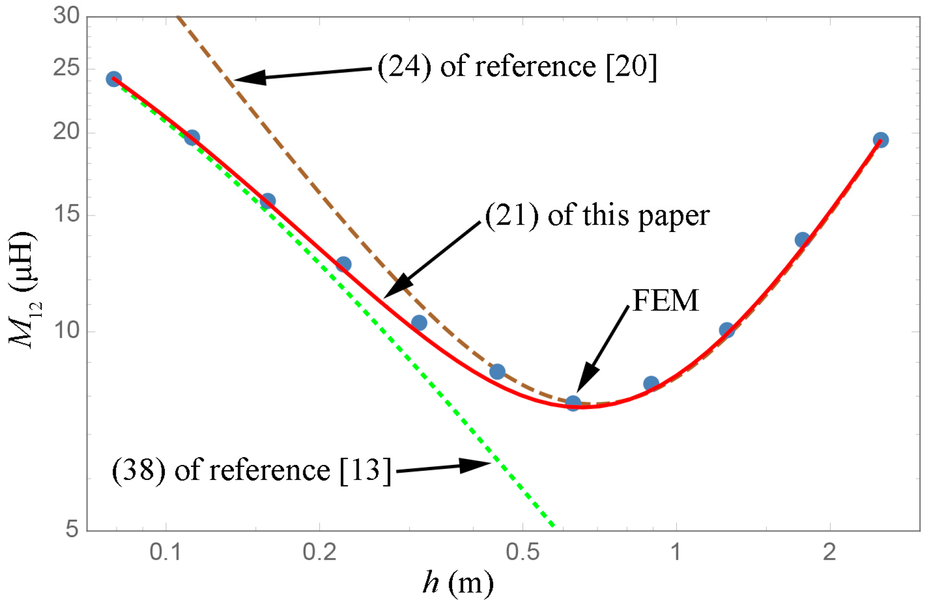
The geometric parameters are listed in

Table 2. Geometric parameters of the coils in Figure 2 (1st comparison).

Parameters	Coil-1	Coil-2
Number of turns	10	10
Pitch length (m)	h	h
Coil length (m)	$10\times h$	$10\times h$
Angular coordinate of the midpoint of the conductor (rad)	0	0
Radius (m)	0.4	0.5

, for the first comparison, in which $b=0$ and the two coils are aligned at the ends. The pitch-length (h) dependence of the mutual inductance is presented in Figure 8.

From Figure 8, it is seen that Equation (21) of this paper is in good agreement with the FEM, for each pitch length (h). Equation (38) of [13] is only valid for a small pitch-length, whereas, Equation (24) of [20] is more suitable for long coils.

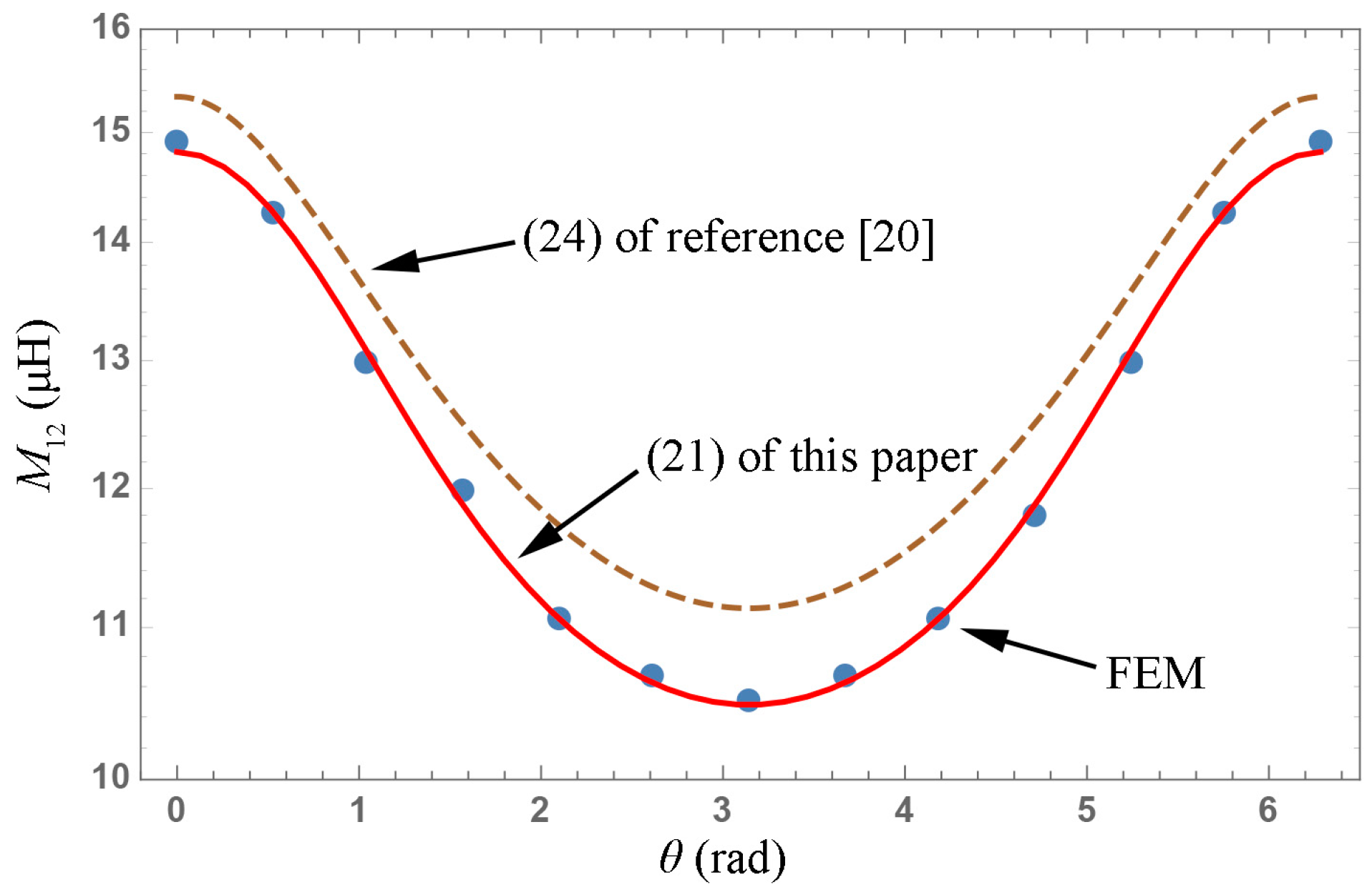
Maintaining the alignment of the coils and $b=0$, the angular coordinate (θ) dependence of the mutual inductance is presented in Figure 9. The geometric parameters are listed in

Table 3. Geometric parameters of the coils in Figure 2 (2nd comparison).

Parameters	Coil-1	Coil-2
Number of turns	10	10
Pitch length (m)	0.629	0.629
Coil length (m)	6.29	6.29
Angular coordinate of the midpoint of the conductor (rad)	0	θ
Radius (m)	0.4	0.5

, for a fixed pitch length (0.629 m).

From Figure 9, it is observed that Equation (21) in this paper is consistent with the FEM result; Equation (24) of [20] is similar to the other two, but some errors continue to exist. Equation (38) of [13] is not suitable for this comparison because it is unaffected by the variation in θ.

The geometric parameters of coils of the third comparison are shown in

Table 4. Geometric parameters of the coils in Figure 2 (3rd comparison).

Parameters	Coil-1	Coil-2
Number of turns	10	10
Pitch length (m)	h	h
Coil length (m)	$10\times h$	$10\times h$
Angular coordinate of the midpoint of the conductor (rad)	0	π
Radius (m)	0.5	0.5

. The ends of the both coils are aligned and the radii are the same. The angular coordinates (θ) of the midpoints of conductor center lines are 0 and π, respectively, and the wires are arranged in a similar manner to the twisted pairs which are common in practice. The pitch-length (h) dependence of the mutual inductance is presented in Figure 10.

When the two coil radii are the same, Equation (38) of [18] cannot be used because the coils are approximated as two overlapping solenoids when using this equation, which leads to calculation program error. It can be seen from Figure 10 that the results of Equation (21) of this paper and FEM are basically the same, and the Equation (24) of [20] is only applicable to the case where the pitch length (h) is large. It is worth noting that the numerical integration of Equation (21) in this comparison converges slowly, which is determined by the intrinsic properties of the modified Bessel functions ($I_{\lambda }\left(va\right)$ and $K_{\lambda }\left(v\rho \right)$).

In the fourth comparison, $b=0$ and the coils remain aligned at the ends. The pitch-length of coil-2 is twice that of coil-1, as specified in

Table 5. Geometric parameters of the coils in Figure 2 (4th comparison).

Parameters	Coil-1	Coil-2
Number of turns	10	5
Pitch length (m)	$h$	$2h$
Coil length (m)	$10\times h$	$5\times 2h$
Angular coordinate of the midpoint of the conductor (rad)	$0$	$\pi$
Radius (m)	0.4	0.5

. The mutual inductances are shown in Figure 11, on varying h.

In the case of unequal pitch lengths, the expressions related to the angular coordinates in Equation (24) of [20] are eliminated. When h is large and the angular coordinates of the midpoint of the conductors are $0$ (coil-1) and $\mathsf{\pi }$ (coil-2), as shown in Table 5, the result of Equation (24) in [20] is similar to those obtained from Equation (21) of this paper and the FEM. However, if coil-2 is rotated by a certain angle around the z-axis, different from Figure 9, the result of Equation (24) in [20] will not change with θ. The general applicability of this formula is lesser than Equation (21) of this paper. Equation (38) of [13] is valid, only when h is small.

Finally, we consider filaments with different heights. One end of each coil is aligned at plane, $z=-6.29/2$, and $b=5\times h-6.29/2$. The other geometric parameters are listed in

Table 6. Geometric parameters of the coils in Figure 2 (5th comparison).

Parameters	Coil-1	Coil-2
Number of turns	10	10
Pitch length (m)	$0.629$	$h$
Coil length (m)	$6.29$	$10\times h$
Angular coordinate of the midpoint of the conductor (rad)	0	0
Radius (m)	0.4	0.5

. The pitch- length (h) dependence of the mutual inductance is presented in Figure 12.

When the heights of the coils are different, Equation (24) of [20] cannot be used. From the other results, it can be observed that Equation (21) of this paper is in good agreement with the FEM results, and Equation (38) of [13] is valid, only when h is small. The curve of Equation (21) of this paper is not smooth, which is an interesting phenomenon. This is because the helical conductors approach and move away, in turn, from each other, as coil-2 is lengthened. The validity of Equation (21) of this paper is verified from the above five comparisons, demonstrating that this equation is suitable for the mutual inductance calculation of finite-length coaxial helical filaments for any geometrical parameter.

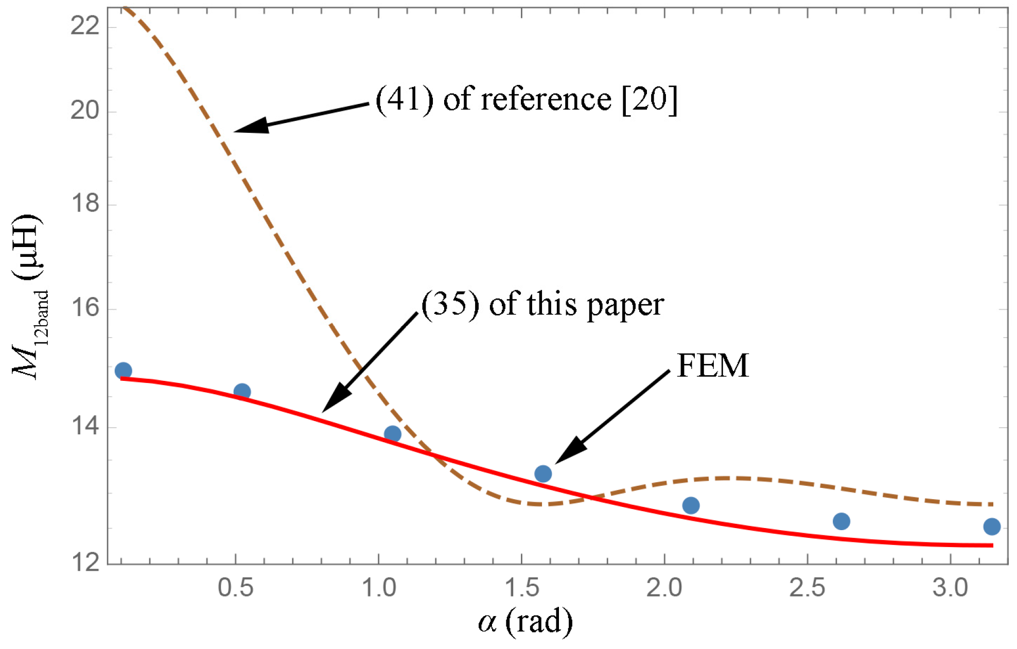
6.2. Comparison with Respect to Finite-Length Coaxial Helical Tape Coils and the Effect of the Inverse Mellin Transform

The geometric parameters of the coils in Figure 3 are listed in

Table 7. Geometric parameters of the coils in Figure 3 (6th comparison).

Parameters	Coil-1	Coil-2
Number of turns	10	10
Pitch length ($\mathrm{m}$)	$0.629$	$0.629$
Coil length ($\mathrm{m}$)	$6.29$	$6.29$
Angular coordinate of the midpoint of the center lines (rad)	0	0
Radius ($\mathrm{m}$)	0.4	0.5

, for comparison between Equation (35) of this paper, Equation (41) of [20], and the FEM. The ends of the coils are aligned, and the angles related to the width of the tape are equal (${\alpha }_1={\alpha }_2=\alpha$). The tape-width ($\alpha$) dependence of the mutual inductance is presented in Figure 13. Similar to the FEM model in Section 6.1, the radial thickness of the coil model for the tape coils is 10 mm, and the radial mid-points of the model are located on the tape conductors, which are treated by analytical calculations. Moreover, as shown in Figure 14, the terminal leads are connected to the ends of the coil center lines.

From Figure 13, it can be observed that Equation (35) of this paper is in good agreement with the FEM; however, there are still certain deviations between Equation (41) of [20] and the above-mentioned two methods. It is worth noting that, when $\alpha$ approaches zero, the calculation result should approach the mutual inductance ($14.82\mathsf{\mu }\mathrm{H}$) of the filaments, with $h=0.629\mathrm{m}$, in Figure 8. However, Equation (41) in [20] does not exhibit this property. In addition, when the mutual inductance of the helical tape coils was derived by integrating the rotation angle of the expression for the mutual inductance of helical filaments, the applicability of the latter Equation (21) to the coil’s geometric parameters was inherited by the former Equation (35); therefore, from the comparisons in Section 6.1, we can see that Equation (35) of this paper has the most general applicability for different geometric parameters, similar to Equation (21).

For twisted pairs of tape conductors which are common in practice, let both coils of Figure 3 have the same radius and the ends aligned, the angles related to the width of the wires are equal to $\frac{\pi }{2}$ (${\alpha }_1={\alpha }_2=\frac{\pi }{2}$). All the geometric parameters are shown in

Table 8. Geometric parameters of the coils in Figure 3 (7th comparison).

Parameters	Coil-1	Coil-2
Number of turns	10	10
Pitch length (m)	$h$	$h$
Coil length (m)	$10\times h$	$10\times h$
Angular coordinate of the midpoint of the center lines (rad)	0	π
Radius (m)	0.5	0.5

. Similar to the third comparison in 6.1, the angular coordinates (θ) of the midpoints of the centerlines are 0 and π, respectively, then the coils are closely wound together. The pitch-length (h) dependence of the mutual inductance are presented in Figure 15.

For the same reason as the third comparison in Section 6.1, Equation (38) of [13] cannot be used. It can be seen from Figure 15 that Equation (35) in this paper is also consistent with the FEM result. The results of Equation (41) in [20] have some deviation from the former two in all cases in Figure 15. Since both coils have the same radius, the numerical integration convergence of Equation (35) is also a bit slow.

When the tape conductors in Figure 3 are closely wound, the inverse Mellin transform can be used for accelerating the calculation speed of the mutual inductance. The geometric parameters are listed in

Table 9. Geometric parameters of the closely-wound coils in Figure 3 (8th comparison).

Parameters	Coil-1	Coil-2
Number of turns	10	10
Pitch length (m)	$h$	$h$
Coil length (m)	$10\times h$	$10\times h$
Angular coordinate of the midpoint of the center lines (rad)	0	0
Radius (m)	0.4	0.5

, with angles of ${\alpha }_1={\alpha }_2=\pi$, for the following comparison. The ends of the coils are also aligned. The pitch-length ($h$) dependence of the mutual inductance are presented in Figure 16. Equation (38) of [13] is used, as in Section 6.1. It can be seen from Figure 16 that the calculation results are the same for Equations (39) and (48) of this paper. Equation (41) of [20] is in good agreement only with the FEM, for large $h$; on the contrary, Equation (38) of [13] is suitable for small pitch lengths alone. FEM verifies the analytical expressions of this paper, in Figure 16.

In order to demonstrate the characteristics of the series obtained by inverse Mellin transform,

Table 10. Pitch length (h) dependence of the time consumption and calculation result between methods of integral and series with different partial sum of the terms.

Pitch Length	h (m)	0.223	0.315	0.445	0.629	0.888
Equation (39) of this paper	Time (ms)	212.6	222.2	217.0	224.6	220.7
	Value (μH)	23.87046728	18.47706415	14.61415102	12.25892005	11.43827601
Equation (48) of this paper (n = 1)	Time (ms)	4.104	4.359	5.733	5.172	4.369
	Value (μH)	23.88430910	18.47956070	14.61459156	12.25899553	11.43828841
Equation (48) of this paper (n = 3)	Time (ms)	5.271	4.710	5.854	5.639	4.213
	Value (μH)	23.87051615	18.47706641	14.61415112	12.25892005	11.43827601
Equation (48) of this paper (n = 5)	Time (ms)	4.704	4.654	5.397	4.603	5.450
	Value (μH)	23.87046768	18.47706416	14.61415102	12.25892005	11.43827601
Equation (48) of this paper (n = 10)	Time (ms)	4.977	4.875	6.529	5.025	4.745
	Value (μH)	23.87046729	18.47706416	14.61415102	12.25892005	11.43827601

gives the calculation results and time consumption of Equations (39) and (48) at some typical points in Figure 16. Among them, the “AccuracyGoal” of the numerical integration was set to 10 in Mathematica, and the series terms selected for sums are: only the first term, the 3 first terms, the 5 first terms and the 10 first terms, all the mutual inductance results were rounded to 10 significant figures. The computer running the analytical calculations has an Intel^® Core™ i5-5257U processor with 1866-MHz DDR3 memory (MacBook Pro, Apple Inc., Cupertino, California, U.S.). From Table 10, we can see that the series in Equation (48) only needs to take the 10 first terms to achieve the same as the first 9 or 10 digits of the numerical integration result, and when the $h$ is large, only 3 terms of the series are required to provide a number which is consistent with the first 10 significant digits of the numerical integration result. It is worth noting that, in most cases, only the first term of the series can lead to a result which fulfills the accuracy requirements of the practical engineering application. The reason why Equation (48) has such a characteristic is that this equation is an asymptotic series with extremely fast convergence. In aspects of time consumption, although the numerical integration has a very high calculation speed (about 200 ms), the series with the same accuracy is faster (about 5 ms) owing to the intrinsic property of itself. Compared to the first two analytical calculation methods, as shown in

Table 11. Pitch length (h) dependence of the time consumption of FEM method.

h (m)	0.223	0.315	0.445	0.629	0.888
FEM (h)	1.286	2.588	3.965	7.256	25.56

, FEM is extremely time consuming, especially when the coil length is long. The FEM was running on a workstation configured as an Intel^® Xeon^® Silver 4110 processor and 2666-MHz DDR4 memory (Precision 7820, Dell Inc., Round Rock, Texas, U.S.), however, the solution time was greater than 25 h and computing resources were considerably occupied.

7. Conclusion

Unlike an ordinary circular coil, a helical coil has arbitrary pitch length. The current in its conductor has components in both the angular and z-axis directions, in a cylindrical coordinate system. In this paper, the actual current direction in helical coils is considered. The mutual inductance of finite-length coaxial filaments was obtained, and the mutual inductance calculation was then generalized for coaxial tape conductors. These expressions were formulated as a series of a single integral of modified Bessel functions, using the series expansion of the reciprocal distance. As there is no approximate processing in the derivation, it is better than the other analytical calculation methods because the expressions presented in this paper are applicable to any corresponding geometric parameters. The direct evaluation of the expressions in this paper is less time-consuming, in software such as Mathematica, which is considerably advantageous compared to FEM. In the case of closely-wound tape conductors, in particular, the series-form expressions of the mutual inductance obtained by inverse Mellin transform can be calculated more rapidly. It was also confirmed that the results obtained in this paper are in good agreement with those obtained by other analytical calculation methods and FEM. The mutual inductance expressions obtained in this paper can be applied in various fields related to helical coils. More generally, the theoretical derivation work in this paper provides valuable tools as a starting point for the analysis of the magnetic field and inductance of helical conductors with other cross-sectional shapes.