Irregular Wave Validation of a Coupling Methodology for Numerical Modelling of Near and Far Field Effects of Wave Energy Converter Arrays

Abstract

Between the Wave Energy Converters (WECs) of a farm, hydrodynamic interactions occur and have an impact on the surrounding wave field, both close to the WECs (“near field” effects) and at large distances from their location (“far field” effects). To simulate this “far field” impact in a fast and accurate way, a generic coupling methodology between hydrodynamic models has been developed by the Coastal Engineering Research Group of Ghent University in Belgium. This coupling methodology has been widely used for regular waves. However, it has not been developed yet for realistic irregular sea states. The objective of this paper is to present a validation of the novel coupling methodology for the test case of irregular waves, which is demonstrated here for coupling between the mild slope wave propagation model, MILDwave, and the ‘Boundary Element Method’-based wave–structure interaction solver, NEMOH. MILDwave is used to model WEC farm “far field” effects, while NEMOH is used to model “near field” effects. The results of the MILDwave-NEMOH coupled model are validated against numerical results from NEMOH, and against the WECwakes experimental data for a single WEC, and for WEC arrays of five and nine WECs. Root Mean Square Error (RMSE) between disturbance coefficient (Kd) values in the entire numerical domain ($RMS{E}_{K_d,D}$) are used for evaluating the performed validation. The $RMS{E}_{K_d,D}$ between results from the MILDwave-NEMOH coupled model and NEMOH is lower than 2.0% for the performed test cases, and between the MILDwave-NEMOH coupled model and the WECwakes experimental data $RMS{E}_{K_d,D}$ remains below 10%. Consequently, the efficiency is demonstrated of the coupling methodology validated here which is used to simulate WEC farm impact on the wave field under the action of irregular waves.

1. Introduction

Ocean waves are an enormous marine renewable energy source with the potential to contribute to a reduction in the world’s fossil fuel dependency. The exploitation of wave energy is a complex and expensive process that takes place in a rough environment. As a result, a large number of Wave Energy Converters (WECs) technologies are under development [1], with none of them yet reaching a commercial stage. In addition, many WECs have to be deployed and arranged in WEC farms to produce large amounts of electricity and to have economically viable wave energy projects.

The overall wave power absorption of a WEC farm will affect the surrounding wave field creating areas of reduced wave energy (areas of decreased wave height) in the lee of the WEC farm as seen in [2,3,4,5,6,7,8]. The hydrodynamic problem of wave power absorption between the WECs within a farm, and between the WECs and the incident wave field is characterized by three different problems namely: wave reflection, diffraction and radiation. The superposition of the reflected, diffracted and radiated wave fields results in a perturbed wave field. The perturbed wave field close to the WECs of the farm caused both by WEC–WEC and wave–WEC interactions is often referred to in literature as the “‘near field” effects while the propagation of this perturbed wave field at a larger distance from the WEC farm e.g., in the coastal zone, is referred to as the “far field” effects [9,10,11,12,13,14,15,16].

Substantial numerical research has been carried out to study the “‘near field” effects in WEC farms, focusing on optimizing the WEC farm layout and maximizing the power output by employing wave–structure numerical models. Typically, numerical models based on potential flow theory have been used either for calculating semi-analytical coefficients [17,18,19] or by means of Boundary Elements Method based models (BEMs) [20,21,22]. The aforementioned numerical models are suited to resolve more accurately the details of WEC (farm) “‘near field” effects. However, they are not able to account for the physical processes that influence the “far field” effects such as wave propagation over a varying bathymetry and wave breaking. Furthermore, the numerical simulation time can increase considerably when increasing the number of WECs modelled and the size of the numerical domain. In recent years, the use of non-linear numerical models based on Computational Fluid Dynamics (CFD) [23,24] and Smoothed Particle Hydrodynamics (SPH) [12,25,26] has increased as these models can take into account non-linear effects for wave–structure interactions. Nonetheless, the use of these models is restricted to a small spatial and temporal scale and to an even more limited number of WECs, which makes them also not suitable to study WEC (farm) “far field” effects in a large numerical domain due to high computational cost.

“Far field” effects are traditionally studied in a computationally cost-efficient way using wave propagation models. In [2,3,4,7,8,27,28,29], phase-averaging spectral models are used to obtain the wave field in the lee of a WEC farm. The WEC farms in these studies are simplified as obstacles which have been assigned a fixed transmission (and thus wave power absorption) coefficient. In a similar way, Refs. [30,31] used a time-dependent mild slope equation model and simplified each WEC as a wave power absorbing obstacle. To obtain the frequency-dependent wave power absorption coefficient for phase-averaging spectral models and the wave power absorption coefficient (assigned to obstacles/structures) for time-dependent mild slope equation models, wave tank testing or numerical modeling are required. Therefore, the simplified parametrization of the wave power absorbed by WECs is not taking into account the wave–structure interactions of diffraction and radiation of the different WECs modelled [32]. This inaccuracy may lead to an overestimation or underestimation of the WEC farm power absorption and consequently an unrealistic estimation of the “far field” effects in the coastal zone.

From the aforementioned studies, it is clear that modeling the perturbed wave field around a farm of WECs is a complex process. Usually “near field” and “far field” effects are approached separately due to the difficulties in using a single numerical model to obtain a fast and accurate solution for both effects. To rectify these limitations, different coupling methodologies between wave–structure interaction solvers and wave propagation models have been developed in the recent years [9,10,11,12,13,14,15]. This allows higher precision in the estimation of “far field” effects, by using a wave–structure interaction solver to obtain an accurate solution of the wave field in a limited area around the WECs of a farm and propagating this resulting wave field further away using a wave propagation model over a coastal zone.

As pointed out in [12], there are different types of coupling methodologies which use one-way and two-way coupling, respectively. In one-way coupled models, there is information transfer in one direction only, where each numerical model is run independently. Examples of such studies, which present linear simulation of “far field” effects of WEC farms by coupling a wave propagation model and a BEM solver, are carried out by [9,10,11,13,33,34]. Alternatively, in two-way coupled models, both numerical models are run at the same time with a two-way transfer of information between them. Examples of two-way coupled models are provided by [12] who demonstrated coupling of a non-linear wave propagation model with an SPH wave–structure interaction solver, or by [35] who simulated a submerged buoy using a non-hydrostatic wave-flow model implemented in the wave propagation model SWASH [36].

In the present study, a continuation of the one-way coupling methodology presented in [13,14,37] for regular waves between the wave propagation model MILDwave [10,38] and the wave–structure interaction solver NEMOH [39] is performed. This coupling methodology is based on the work of [9,38], who first presented a coupling between a wave propagation model (MILDwave) and a wave–structure interaction solver WAMIT [40]. In [14] specifically, the step-by-step procedure of this coupling methodology is presented and its application range. Moreover, in [14], the theoretical background of both the coupling methodology and of the employed numerical models (MILDwave and NEMOH) is provided. Furthermore, in [14], experimental data from the “WECwakes” database [41] has been used and more specifically wave field measurements for a 9-WEC array interacting with the incoming waves. The latter was used to perform validation of the coupling methodology for regular waves propagating through the 9-WEC array, obtaining good agreement between the experimental and numerical results regarding the impact of the 9-WEC array on the surrounding wave field. In [14], irregular waves were briefly introduced, yet not validated, without presenting a fully developed coupling methodology for irregular wave simulations.

Here, the novelty of this study is the validation of a fully developed coupling methodology for modeling irregular waves using available experimental data [16,41]. In the present manuscript, the coupling methodology is presented in detail for irregular wave generation. Furthermore, the irregular wave cases of a 9-WEC array, a 5-WEC array and a single WEC are selected from the “WECwakes” database for simulations using the coupling methodology and for validation purposes. Moreover, numerical results of the MILDwave-NEMOH coupled model are compared to NEMOH numerical results and experimental data, showing that the coupled model is able to accurately parse the information between the NEMOH and MILDwave numerical domains in the “near field”. This information is then propagated into the “far field” in the MILDwave numerical domain as MILDwave correctly models coastal transformations [42]. Based on the results from [14] and on the current results from the present work, it is demonstrated that the developed and validated coupling methodology can be a useful tool for cost-efficient computational time simulations of coastal impacts of farms of floating structures and WECs over a large coastal zone. In contrast, it should also be noted that, due to the limitations of the numerical models employed here, the resulting MILDwave-NEMOH coupled model cannot be used for non-linear sea states and to model morphological coastal impacts.

The structure of the paper is as follows: Section 1 provides a short overview of the state-of-the-art and problem statement. Section 2 presents a description of the generic coupling methodology. Section 3 illustrates the MILDwave-NEMOH coupled model, including a detailed description of the coupling methodology implementation, the wave propagation solver MILDwave and the wave–structure interaction solver NEMOH. A validation test case is described in Section 4 and the results are presented in Section 5. In Section 6, the capability of the "MILDwave-NEMOH" coupled model to simulate “far field” effects of WEC farms is discussed. Finally, the conclusions of this and future work are drawn in Section 7.

2. Generic Coupling Methodology

In this section, the generic coupling methodology first introduced by [9] is briefly presented. The objective of the coupling methodology is to obtain the total wave field around a (group of) structure(s), as a superposition of the incident wave field and the perturbed wave field (which is a combination of the reflected, diffracted and radiated wave fields). The incident wave field propagation and transformation is calculated over a large domain using a wave propagation numerical model. The perturbed wave field is simulated using a wave–structure interaction solver over a restricted domain around the structure(s), namely the coupling region. As it has been pointed out in [9], this coupling methodology can be applied by employing any wave–structure interaction solver that describes the perturbed wave field, any wave propagation model and any type of oscillating or floating structure(s).

The general strategy for the coupling methodology has been also recently reported and updated in [14], but, for clarity, it is presented here briefly. It consists of four steps. Firstly (Step 1), a wave propagation model is used to obtain the incident wave field at the location of the structure(s) when the structure(s) is (are) not present. Secondly (Step 2), the obtained wave field from Step 1 is used as an input for the wave–structure interaction solver at the location of the structure(s). Then, the motion of the structure(s) is solved and an accurate solution of the perturbed wave fields around the structure(s) is obtained. Thirdly (Step 3), the perturbed wave field is used as an input in the wave propagation model and is propagated throughout a large domain. This is done by prescribing an internal wave generation boundary around the structure location. Finally (Step 4), the total wave field due to the presence of the structure(s) is obtained as the superposition of the incident wave field and the perturbed wave field in the wave propagation model.

3. Application of the Coupling Methodology between the Wave Propagation Model, MILDwave, and the Wave–Structure Interaction Solver NEMOH for Irregular Waves

In this section, the generic coupling methodology presented in Section 2 will be demonstrated for coupling between the wave propagation model MILDwave and the wave–structure interaction solver NEMOH. First, a description of the two numerical models employed is presented. Subsequently, a description of the irregular wave generation for the incident, perturbed and total wave fields is provided.

3.1. The Wave Propagation Model, MILDwave and the Wave–Structure Interaction Solver, NEMOH

The wave propagation model chosen for demonstrating the proposed coupling methodology is the mild slope model MILDwave [10,38], developed at the Coastal Engineering Research Group of Ghent University, in Belgium. MILDwave is a phase-resolving model based on the depth-integrated mild slope equations of Radder and Dingemans [43]. MILDwave allows for solving the shoaling and refraction of waves propagating above mild slope varying bathymetries, and it has been widely used in the modeling of WEC farms [10,11,13,30,31,41,44,45]. The basic MILDwave equations are reported in [10].

The wave–structure interaction solver chosen to solve the diffraction/radiation problem is the open-source potential flow BEM solver NEMOH, developed at Ecole Centrale de Nantes [39]. Linear potential flow theory has hitherto been utilized in a majority of the investigations into WEC array modeling—for example, see [11,19,46,47]. NEMOH is based on linear potential flow theory [48], and the basic equations and assumptions employed are reported in [14].

3.2. Generation of the Incident Wave Field for Irregular Waves

Irregular waves can be generated by applying the superposition principle of a number of different linear regular wave components. The incident wave field for a linear regular wave is generated intrinsically in MILDwave. Moreover, MILDwave allows for solving shoaling and refraction of waves propagating over complex bathymetries. The numerical set-up of MILDwave is illustrated in Figure 1. Waves are generated along a linear offshore wave generation boundary by applying the boundary condition of linear regular waves generation:

$${\eta }_{I,reg}(x,y,t)=acos(\omega t-k(xcos\left(\theta \right)+ysin\left(\theta \right))),$$

(1)

where ${\eta }_{I,reg}$ is the incident regular wave surface elevation, a is the wave amplitude, $\omega$ is the angular frequency, k is the wave number and $\theta$ is the wave direction. To minimize unwanted wave reflection, absorption layers are placed down-wave and up-wave in the numerical wave basin.

By applying the superposition principle, a first order irregular wave is represented as the finite sum of N regular wave components characterized by their wave amplitude, $a_j$, and wave period, $T_j$, derived from the wave spectral density, $S_j$:

$${\eta }_{I,irreg}(x,y,t)=\sum _{j=1}^N{a}_{j}cos({\omega }_{j}t-k_j(xcos\left({\theta }_j\right)+ysin\left({\theta }_j\right))+{\phi }_j),$$

(2)

where

$$a_j=\sqrt{2S_j\left(f_j\right)·\Delta f_j},$$

(3)

where ${\eta }_{I,irreg}$ is the incident irregular wave surface elevation and $a_j$ is the wave amplitude, ${\omega }_j$ is the wave angular frequency, $f_j$ is the wave frequency, $k_j$ is the wave number, ${\theta }_j$ is the wave direction and ${\phi }_j$ is the incident phase, of each wave frequency component. ${\phi }_j$ is selected randomly between $-\pi$ and $\pi$ to avoid local attenuation of ${\eta }_{I,irreg}$.

3.3. Generation of the Perturbed Wave Field for Irregular Waves

To calculate the irregular perturbed wave field around a (group of) structure(s) first, it is necessary to obtain the perturbed wave field for each wave frequency as a regular wave. The perturbed wave field in the time domain for a regular wave is obtained in two steps and the generic numerical set-up is illustrated in Figure 1. First, a frequency-dependent simulation is performed using NEMOH to obtain the complex perturbed wave field around the (group of) structure(s). NEMOH resolves the wave frequency-dependent wave radiation problem for each structure(s) and the diffraction (including radiation) over a predetermined numerical grid with the wave phase $\phi =0$ at the center of the domain. The resulting radiated and diffracted wave fields for each wave frequency depend on the shape and number of floating structure(s), the number of Degrees of Freedom (DOF) considered, the local constant water depth and the wave period.

The radiated (for each structure) and diffracted (for all structures) complex wave fields in NEMOH are summed up to obtain the perturbed wave field, ${\eta }_{pert}$:

$${\eta }_{pert}={\eta }_{diff}+{\eta }_{rad},$$

(4)

where ${\eta }_{rad}$ is the radiated wave field and ${\eta }_{diff}$ is the diffracted wave field.

Secondly, the perturbed wave field is transformed from the frequency domain to the time domain and imposed onto MILDwave using an internal wave generation boundary (Figure 1). For this study, a circular wave generation boundary is prescribed; however, it can be defined using other shapes as well. Waves are forced away from the circular wave generation boundary by imposing values of free surface elevation ${\eta }_{circ}(x,y,t)$ as described by Equation (5):

$${\eta }_{circ}(x,y,t)=a_c\left|{\eta }_{pert}\right|cos({\phi }_{pert,c}-\omega t),$$

(5)

where ${\eta }_{pert}$ is the perturbed complex wave field in the circular wave generation boundary, and $a_c$ and ${\phi }_{pert,c}$ are the wave amplitude of the incident wave and the wave phase of the perturbed wave at the center of the circular wave generation boundary, respectively. To avoid unwanted wave reflection, wave absorption layers or relaxation zones are implemented up-wave, down-wave and also in the sides of the MILDwave numerical domain (Figure 1).

As in the case for the calculation of the irregular incident wave field, the irregular perturbed wave field is calculated as the finite sum of N regular perturbed wave components characterized at the center of the wave generation boundary by their wave amplitude, $a_{c,j}$, derived from the wave spectrum:

$${\eta }_{pert,irreg}(x,y,t)=\sum _{j=1}^N{a}_{c,j}\left|{\eta }_{pert}\right|cos({\phi }_{pert,c,j}-{\omega }_{j}t),$$

(6)

where

$$a_{c,j}=\sqrt{2S_{c,j}\left(f_j\right)·\Delta f_j}$$

(7)

and ${\eta }_{pert,irreg}$ is the perturbed irregular wave surface elevation where $S_{c,j}$ is the spectral density and ${\phi }_{pert,c,j}$ is the perturbed wave phase of each frequency component. ${\phi }_{pert,c,j}$ is selected randomly between $-\pi$ and $\pi$ to avoid local attenuation of the surface elevation.

3.4. Generation of the Total Wave Field for Irregular Waves

The total wave field for irregular waves due to the presence of a (group of) structure(s) is obtained by applying the generic coupling methodology described in Section 2. This is performed by superimposing the irregular incident wave field and the irregular perturbed wave field generated in MILDwave as shown in Section 3.2 and Section 3.3, respectively.

Step 1 of the generic coupling methodology is applied N times for irregular waves to calculate the incident wave field for N regular wave components in MILDwave by applying a random phase ${\phi }_i$ for each simulation. From each simulation $a_{c,i}$, and ${\phi }_{c,i}$ are obtained at the center of the circular wave generation boundary and are used as input values for NEMOH.

In Step 2, the perturbed wave field is obtained in NEMOH. In NEMOH, ${\phi }_{pert,c,j}$ is referenced with respect to the center of the domain (Section 3.3). Therefore, ${\phi }_{pert,c,j}$ at the NEMOH numerical domain has to be corrected using the ${\phi }_j$ of the regular incident wave field to assure wave phase matching between the incident and the perturbed waves in MILDwave.

Afterwards, in Step 3, the perturbed wave field is then transformed from the frequency domain to the time domain and propagated into MILDwave for N regular perturbed wave components along the circular wave generation boundary.

Finally, in Step 4, the irregular incident wave field is obtained as the superposition of the N incident regular waves simulations from Step 1. The irregular perturbed wave field is obtained as the superposition of the N perturbed regular wave simulations from Step 3. The total wave field for irregular waves is obtained as the combination of the irregular incident and perturbed wave fields:

$${\eta }_{tot,irreg}(x,y,t)=\sum _j^N{\eta }_{I,reg,j}(x,y,t)+\sum _j^N{\eta }_{pert,reg,j}(x,y,t),$$

(8)

where ${\eta }_{tot,irreg}$ is the total irregular wave surface elevation, and ${\eta }_{I,reg,j}$ and ${\eta }_{pert,reg,j}$ are the incident and perturbed wave surface elevations of each wave frequency, respectively.

4. Validation Strategy of the Coupling Methodology between the Wave Propagation Model, MILDwave, and the Wave–Structure Interaction Solver, NEMOH

In this section, a validation test case is presented to validate the MILDwave-NEMOH coupled model against numerical results from NEMOH and experimental data. Showing that the perturbed wave field can be precisely parsed from the NEMOH to the MILDwave domain in the near field of the WEC array. The criteria evaluated for the numerical model validation are also described.

4.1. Validation Test Cases

The validation of the demonstrated generic coupling methodology is carried out by comparing the results from the MILDwave-NEMOH coupled model to those obtained from the numerical model NEMOH and the WEC array experimental data from the WECwakes project [9,16,41].

4.1.1. WECwakes Experimental Data-Set

This section gives a short description of the experimental data-set from the WECwakes project [9,16,41] conducted in the Shallow Water Wave Basin of DHI, Hørsholm (Denmark). In the WECwakes project, arrays up to 25 point absorber type WECs (cylinders of a diameter of 0.315 m) were tested to study “near field” and “far field” effects of heaving point absorber type WECs. A Coulomb friction based damping is used.

The DHI wave basin is 22 m wide and 25 m long and the overall water depth is fixed to 0.7 m. Different WEC array configurations have been tested during the WECwakes project under a wide range of sea states, a large experimental data-set has been generated and is publicly available for numerical validation purposes and for WEC array design guidelines. The wave field around the WECs has been recorded using 41 resistive wave gauges (WGs) distributed in the wave basin.

For the present validation study, three different WEC configurations are selected: a single WEC, an array of five WECs arranged in a 1 × 5 WEC layout and an array of nine WECs arranged in a 3 × 3 WEC layout (see Figure 1B–D). A total of 15 wave gauges located in the front, leeward and sides of the WECs array configurations are used to compare the significant wave height, $H_s$, and the spectral density, S, between the MILDwave-NEMOH coupled model and the experimental data-set. The separating distance between the different WECs is equal to 1.575 m (centre-to-centre distance). The incident irregular wave conditions used to generate waves during the experiments test are defined by a JONSWAP spectrum with $H_s=0.104$ m and two peak wave periods of $T_p=1.18$ s and $1.26$ s.

4.1.2. “Test Case” Program

The primary objective of the present research is to validate the total wave field around a WEC array obtained using the MILDwave-NEMOH coupled model. For this reason, a “Test Case” (

Table 1. “Test Case” program for irregular waves, and different Wave Energy Converter (WEC) (array) configurations.

Test Case	Significant Wave	Peak Wave	Water Depth,	WEC Buoy	WEC (Array)
Number ♯	Height, ${\mathit{H}}_{\mathit{s}}$ (m)	Period, ${\mathit{T}}_{\mathit{p}}$ (s)	d (m)	Motion (-)	Layout (-)
1	0.104	1.18	0.700	Damped	1 × 1
2	0.104	1.26	0.700	Damped	1 × 1
3	0.104	1.26	0.700	No motion (fixed buoy)	1 × 5
4	0.104	1.26	0.700	Damped	1 × 5
5	0.104	1.18	0.700	Damped	3 × 3
6	0.104	1.26	0.700	Damped	3 × 3

) program based on the WECwakes experimental data-set has been designed for different irregular wave cases and WEC (array) configurations:

The different “Test Cases” included in Table 1 are performed both using the MILDwave-NEMOH coupled model, and NEMOH. NEMOH simulation results are used: (1) as input for the MILDwave-NEMOH coupled model, and (2) as a benchmark for the validation of the MILDwave-NEMOH coupled model, which is also compared with WECwakes data.

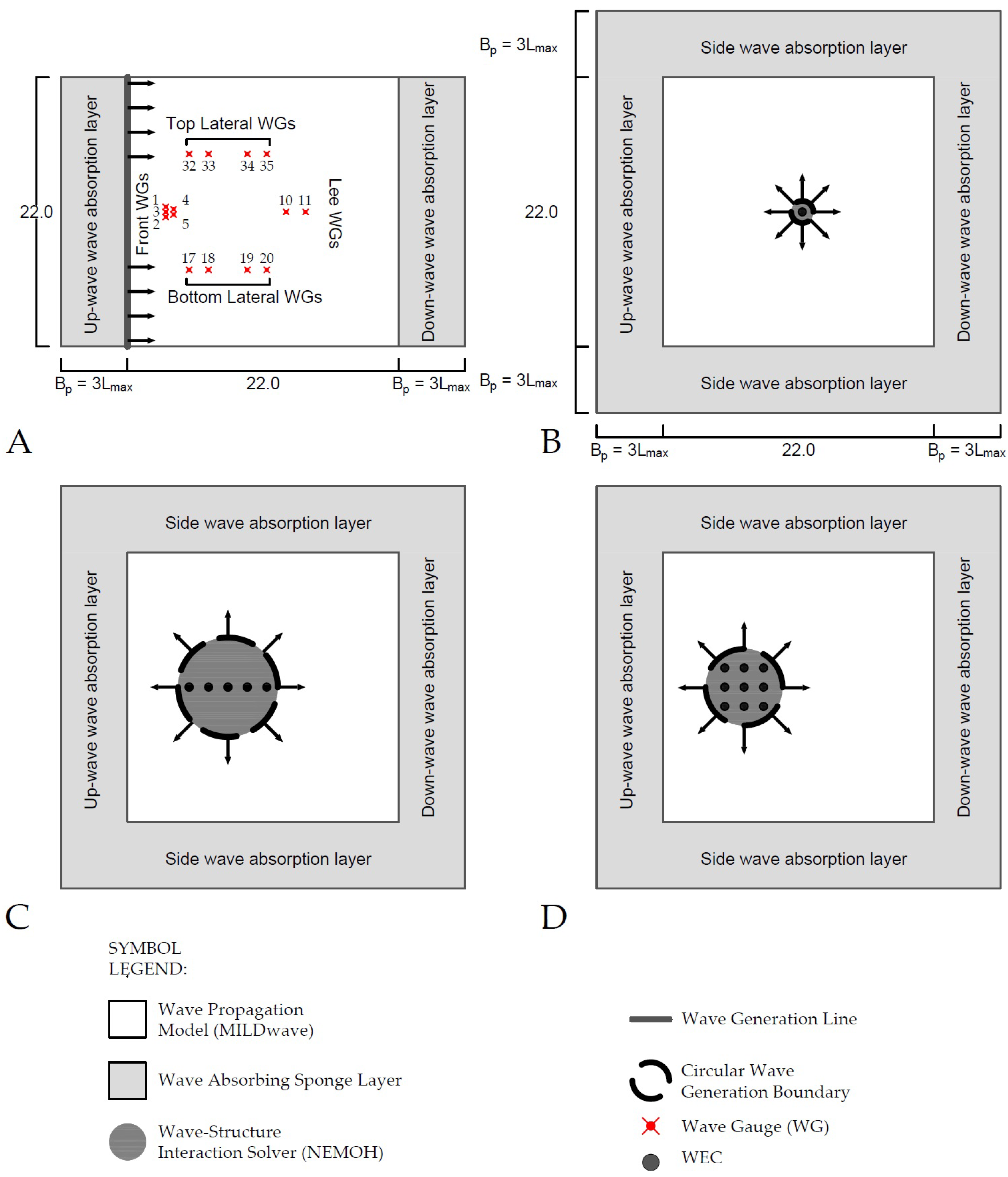
4.1.3. Numerical Set-Up in the Used Models

In MILDwave, simulations are carried out in two types of numerical wave basins (see Figure 1A–D) with an effective domain (area not covered by the wave absorbing sponge layers) of 22 m width and 22 m length, and a constant water depth of 0.700 m. The same dimensions are used in NEMOH. Four equally sized effective numerical domains are used. For the simulations performed to obtain the incident wave field, waves are generated using a linear wave generation line located on the left side of the numerical domain with two equally sized wave absorbing sponge layers placed up-wave (left) and down-wave (right) (see Figure 1A).

For the simulations carried out to obtain the perturbed wave field, waves are generated using an internal circular wave generation boundary (Figure 1B–D). The three different WEC (arrays) configurations of Table 1 are simulated using different coupling radii for the circular wave generation boundary (see Figure 1B–D). Each coupling radius is obtained following the recommendations by [11] as $0.5$ times the wave length (L) plus the radius of the WEC or the distance from the centre of the circular area to the most distant WEC for a single WEC and a WEC array, respectively. Four equally sized wave absorbing sponge layers are placed on all sides of the numerical domain.

The dimensions of the total numerical wave basin in MILDwave are not always the same, as the length of the wave absorbing sponge layers (B) is different for each set of wave conditions and depends on L. As irregular waves are obtained as a superposition of $N_f$ regular wave components, B is calculated using $L_{max}$, which corresponds to $T_{max}$ of the discretized spectra. An increase of B causes a decrease of wave reflection, and as pointed out in [5] for $B=3·L_{max}$ wave reflection coefficient drops to 1%.

The total wave field of the MILDwave-NEMOH coupled model is obtained as the superposition of the numerical results from the domains of Figure 1A–D for a single WEC, five WECs and nine WECs, respectively.

In NEMOH, the effect of the WEC’s Power Take-Off (PTO) system is taken into account by adding a suitable external damping coefficient, $B_{PTO}$ = 28.5 kg/s as defined in [14].

4.2. Criteria Used for the Numerical Model Validation

The accuracy of the obtained numerical results is evaluated in two steps. Firstly, results from the MILDwave-NEMOH coupled model are compared against the NEMOH results. Secondly, results from the MILDwave-NEMOH coupled model are compared against WECwakes experimental data.

The comparison between the MILDwave-NEMOH coupled model and NEMOH is assessed by calculating $K_d$ coefficient values, as defined in Equations (9) and (10), respectively. The $K_d$ coefficient is defined as the ratio between the numerically calculated local total significant wave height, $H_{s,tot}$, and the target incident significant wave height, $H_{s,I}$, imposed along the linear wave generation boundary. In the MILDwave-NEMOH coupled model, the $K_{d,coupled}$ is obtained in the time domain as:

$$K_{d,coupled}=\frac{H_{s,tot}}{H_{s,I}}=\frac{4·\sqrt{{\sum }_t^{\Delta t}{({\eta }_{I,irreg,t}+{\eta }_{pert,irreg,t})}^2·\frac{dt}{\Delta t}}}{H_{s,I}},$$

(9)

where ${\eta }_{I,irreg,t}$ and ${\eta }_{pert,irreg,t}$ are the free surface elevations for irregular incident and perturbed waves in each time step $dt$, from the domains of Figure 1A–D, respectively, and $\Delta t$ is the time window over which $K_d$ is computed. In NEMOH, the $K_{d,NEMOH}$ is obtained in the frequency domain as:

$$K_{d,NEMOH}=\frac{\left|{\eta }_{tot,irreg,freq}\right|}{H_{s,I}},$$

(10)

where $\left|{\eta }_{tot,irreg,freq}\right|$ is the absolute value of free surface elevation for the complex total wave obtained in the frequency domain.

The $K_d$ value is a useful parameter that has been used extensively in literature to study wave field variations [9,10,11,22,31,34,42,45]. $K_d$ > 1 and $K_d$ < 1 indicate increase and decrease of the local wave height, respectively. When studying WEC arrays, increases in the local wave height indicate the presence of “hot spots” [49], defined as areas of high wave energy concentration. Instead, decrease in the local wave height denotes "wake" effects, which result in an area of reduced wave energy.

To evaluate $K_d$ differences between the MILDwave-NEMOH coupled model and NEMOH, three different outputs have been generated:

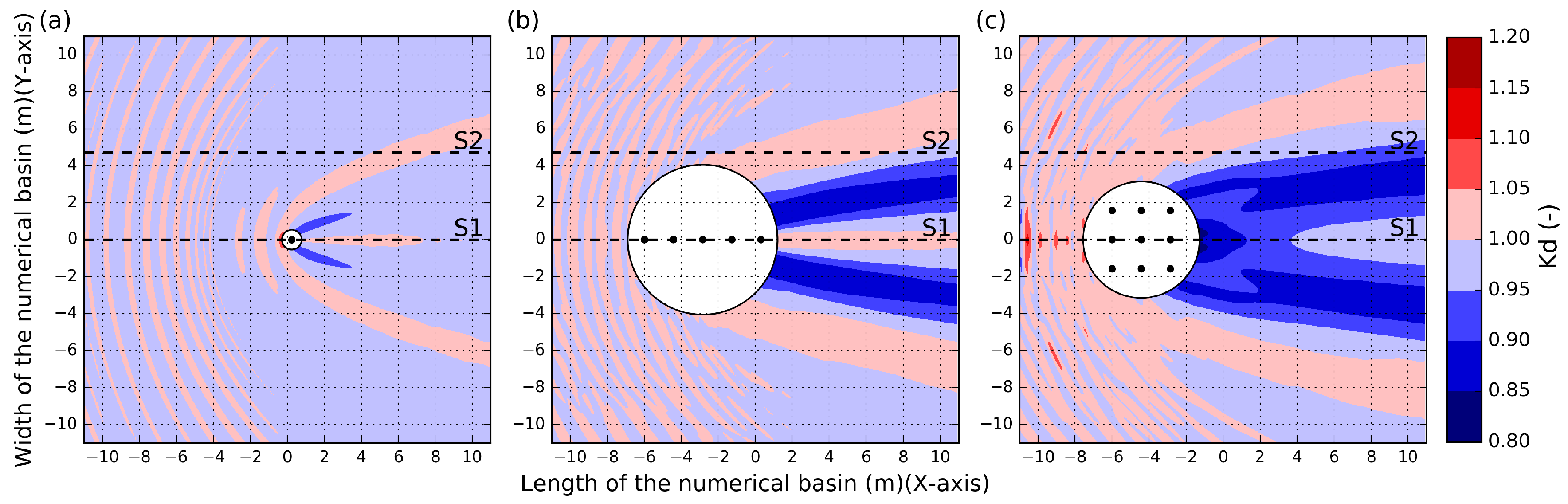
• $K_d$ contour plots of the entire numerical domains;
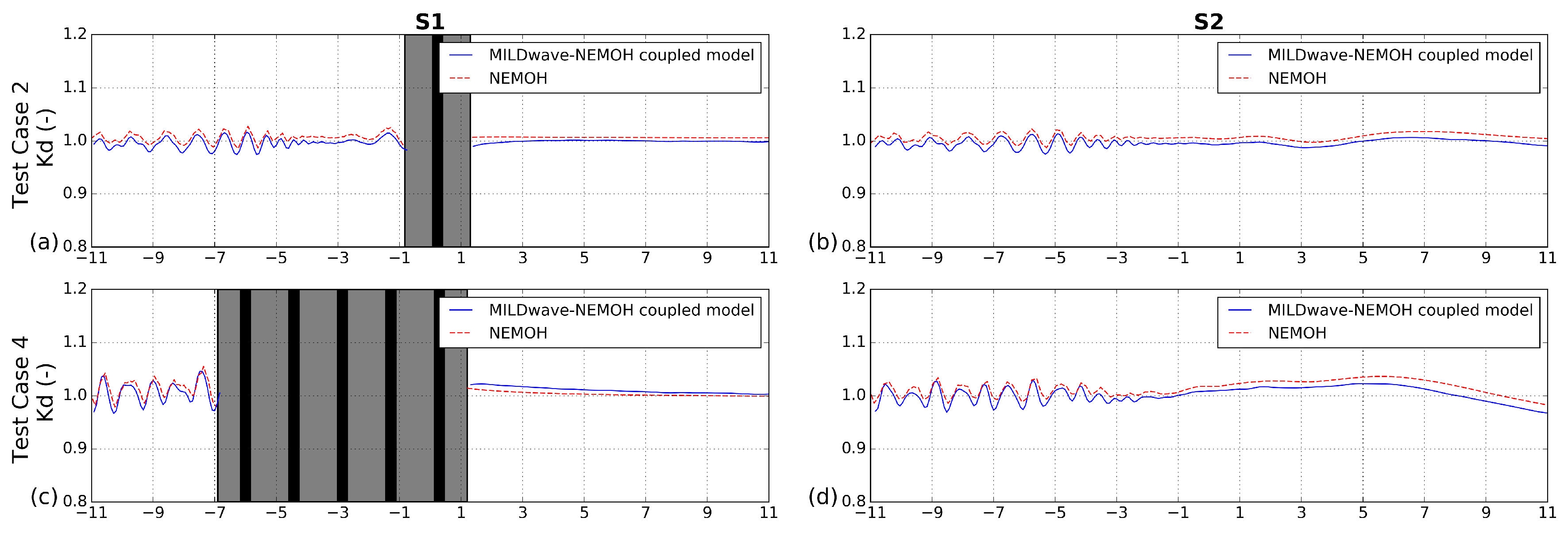
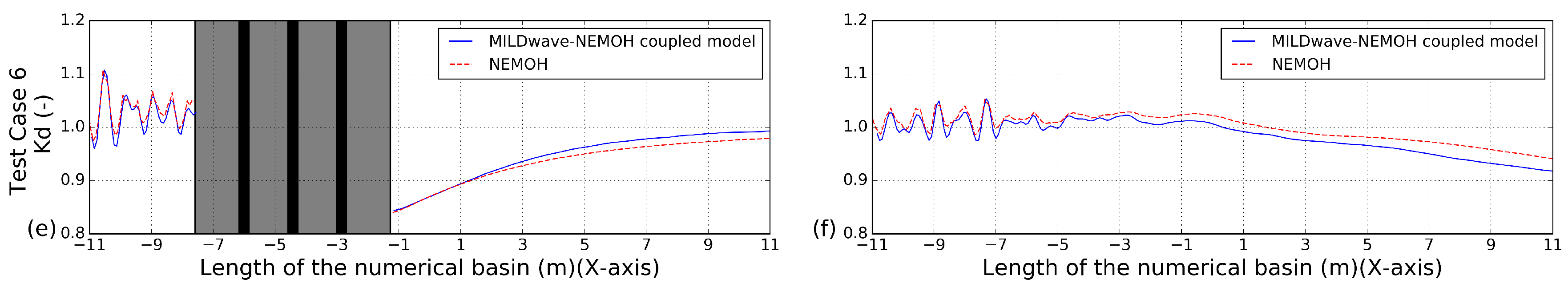
• $K_d$ cross-sections along the length of the numerical domains (parallel to the wave propagation direction);
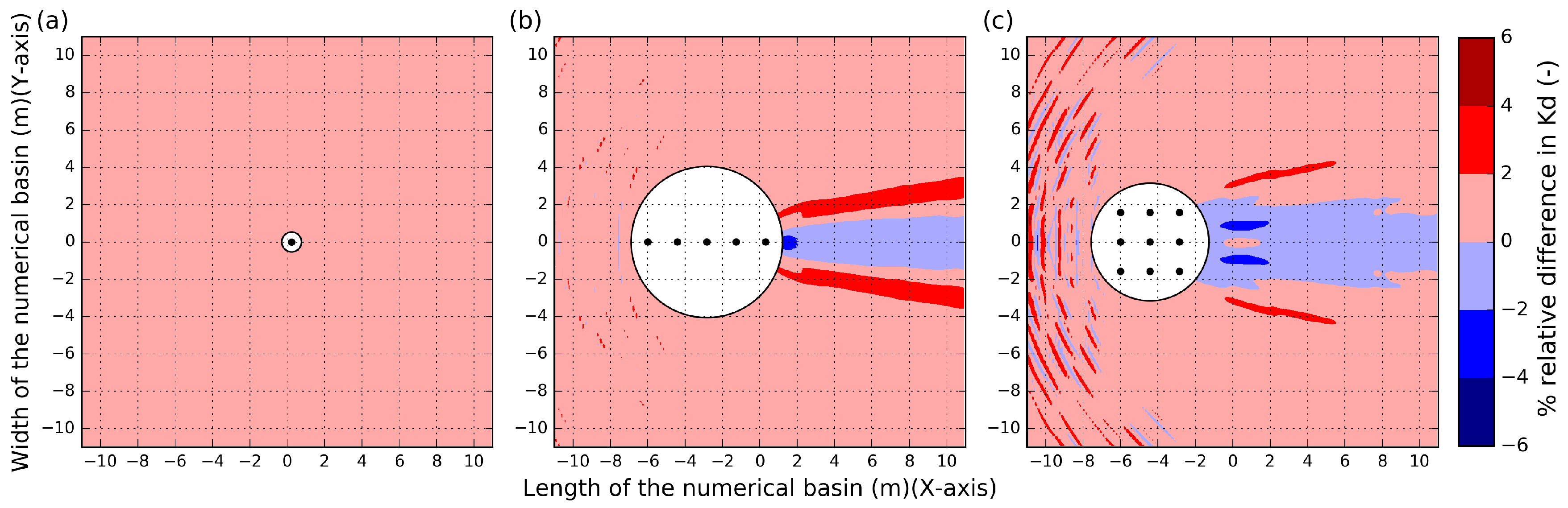
• Contour plots of the “Relative Difference” between the obtained $K_d$ values ($R{D}_{K_d}$) defined as:

  $$R{D}_{K_d,D}=\frac{(K_{d,NEMOH}-K_{d,coupled})}{K_{d,NEMOH}}·100\%(-),$$

  (11)
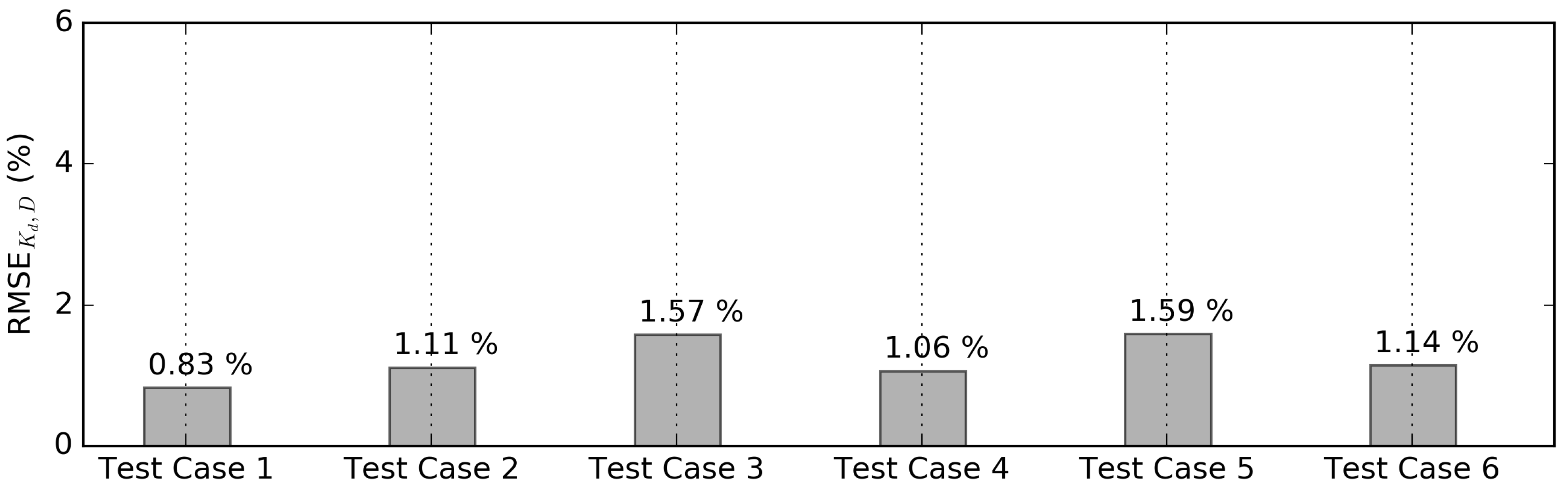
• The Root Mean Square Error between $K_d$ values obtained using the MILDwave-NEMOH coupled model and NEMOH for the entire numerical domain ($RMS{E}_{K_d,D}$):

  $$RMS{E}_{K_d,D}=\sqrt{\frac{{\sum }_{i=1}^G{(K_{d,NEMOH}-K_{d,coupled})}^2}{G}}·100\%(-),$$

  (12)

  where G is the number of grid points of the numerical domain (D).

The validation of results obtained from the MILDwave-NEMOH coupled model against WECwakes experimental data is carried out using data recorded at the 15 numerical and experimental WGs, respectively, as these are illustrated in Figure 1A. For each WG, two different outputs have been generated:

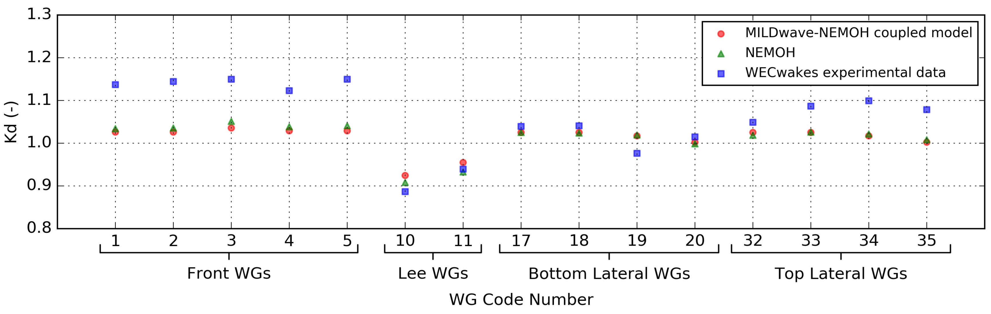
• Spectral density plots comparing the wave spectra between the MILDwave-NEMOH coupled model and the WECwakes experimental data for the 15 WGs.
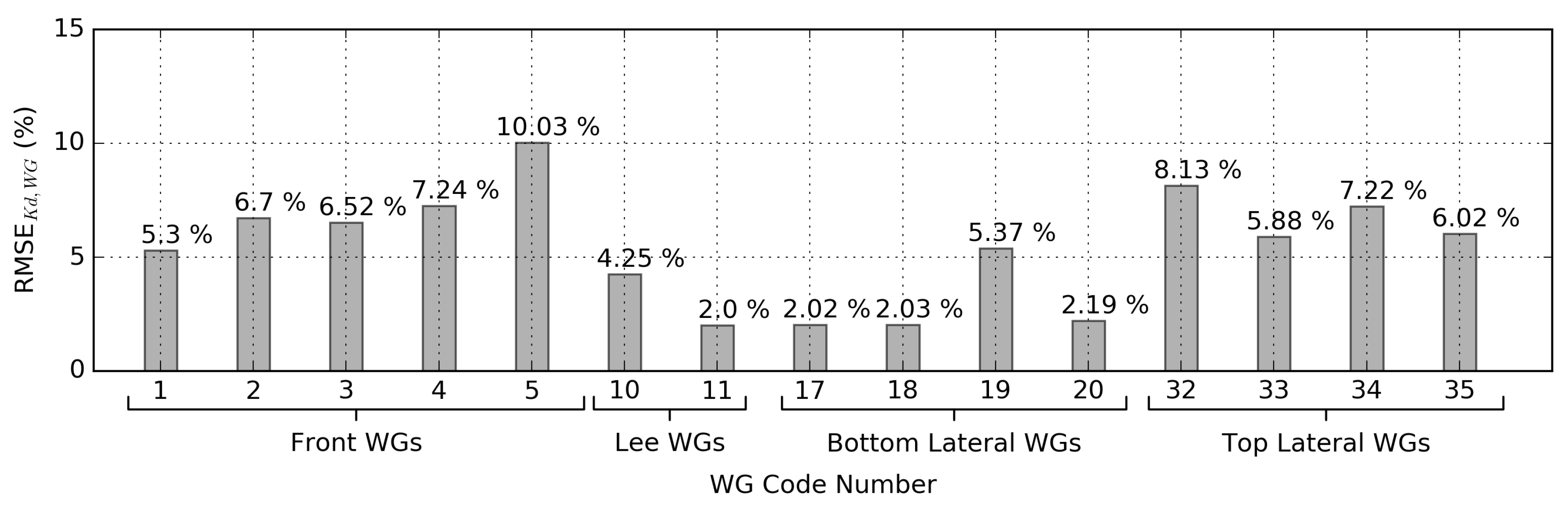
• The Root Mean Square Error between the $K_d$ of the MILDwave-NEMOH coupled model and the $K_{d,WECwakes}$ of the WECwakes experimental data for the 15 WGs, $RMS{E}_{K_{d,WG}}$:

  $$RMS{E}_{K_{d,WG}}=\sqrt{\frac{{\sum }_{i=1}^T{(K_{d,WECwakes}-K_{d,coupled})}^2}{C}}·100\%(-),$$

  (13)

  where C is the number of Test Cases.

5. Validation Results

In Section 5.1, the results for the irregular wave generation analysis are presented. The comparison between the MILDwave-NEMOH coupled model and NEMOH follows in Section 5.2. First, the results for Test Case 6 are discussed in detail in Section 5.2.1, and then the results for all Test Cases are summarized in Section 5.2.2 in terms of $RMS{E}_{K_d,D}$ values. The validation between the MILDwave-NEMOH coupled model and the WECwakes experimental data is included in Section 5.3. Similarly, first, the results for Test Case 6 are discussed in detail in Section 5.3.1, while the results for all Test Cases are summarized in Section 5.3.2 in terms of $RMS{E}_{K_d,D}$ values.

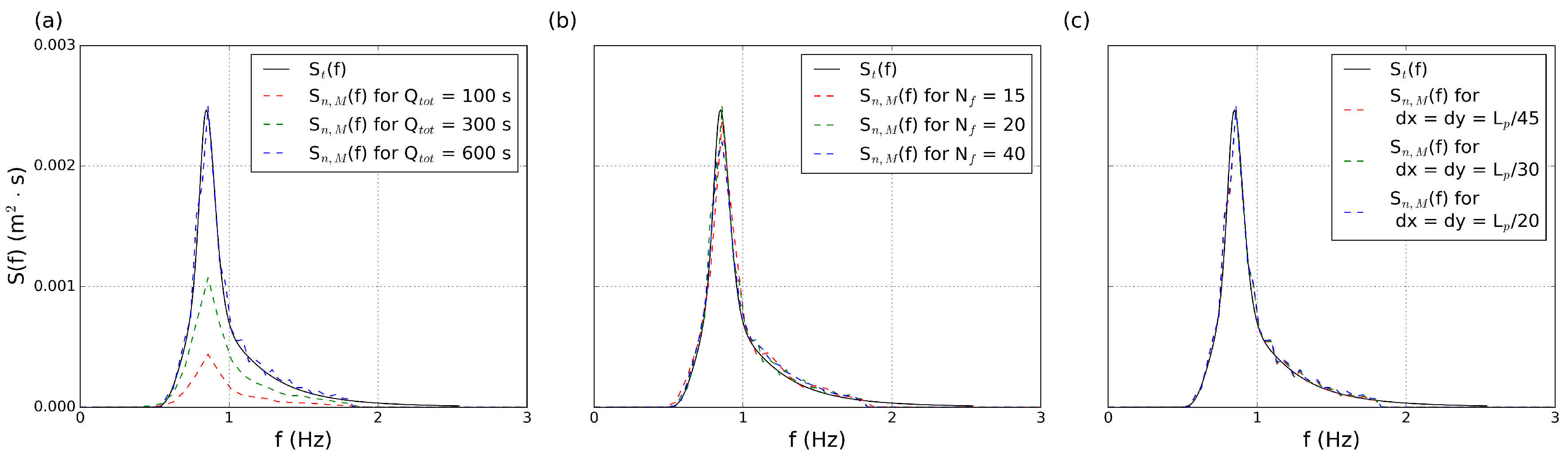
5.1. Sensitivity Analysis for Irregular Wave Generation

Before performing the numerical simulations listed in Table 1, a sensitivity analysis is carried out to ensure a converging result of the irregular wave simulation, while keeping the computational time low. This sensitivity analysis is based on three numerical simulation criteria: (1) the total simulation time $Q_{tot}$, (2) the number of regular wave components ($N_f$), and (3) the grid cell size ($d_x$ and $d_y$) employed in MILDwave. For each criterium, the studied parameter is varied while the other two are kept constant. The numerical domain in Figure 1A is used.

Firstly, different $Q_{tot}$ are considered to ensure a fully developed wave spectrum. Secondly, $N_f$ is modified in order to achieve a wave spectrum close to the theoretical one. Thirdly, $d_x=d_y$ is varied based on wave length, $L_p$ of the incident waves in order to achieve a convergent solution with the theoretical spectral density $S_t\left(f\right)$. The numerical spectral density in MILDwave $S_{n,M}\left(f\right)$ is obtained at the centre of the domain for the incident wave of “Test case 1” of Table 1. The shortest $Q_{tot}$, smallest $N_f$ and largest $d_x=d_y$ resulting in an accurate solution of $S_{n,M}\left(f\right)$ are selected then to perform the rest of the numerical simulations for the rest of the Test Cases.

The results of the irregular wave generation sensitivity analysis are shown in Figure 2. $S_{n,M}\left(f\right)$ for different $Q_{tot}$ is plotted in Figure 2a, while $N_f$ = 15 and the $d_x=d_y=0.08$ m are kept constant. It is clearly observed that, for $Q_{tot}$ of 100 s and 300 s, $S_{n,M}\left(f\right)$ does not represent $S_t\left(f\right)$. For $Q_{tot}$ of 600 s, there is a good agreement with $S_t\left(f\right)$ even for high frequency wave components, without leading to computationally expensive simulations.

$S_{n,M}\left(f\right)$ for different $N_f$ is compared to $S_t\left(f\right)$ in Figure 2b, while $Q_{tot}$ = 600 s and the $d_x=d_y=0.08$ m are kept constant. Simulations are performed for $N_f$ = 15, 20 and 40. There is a good agreement between $S_{n,M}\left(f\right)$ and $S_t\left(f\right)$ for all three simulations showing a slight amount of spurious energy for high wave frequencies, which is reduced by increasing $N_f$. Nevertheless, the accuracy gained by increasing $N_f$ from 20 to 40 is not significant as the $S_{n,M}\left(f\right)$ peak and the energy contained within the $S_{n,M}\left(f\right)$ curve is practically the same. Consequently, it is concluded that increasing $N_f$ is not required and therefore $N_f$ is kept to 20 to reduce the computational time.

To complete the sensitivity analysis, $S_{n,M}\left(f\right)$ for different $d_x$ (where $d_x=d_y$) is compared in Figure 2c, while keeping $Q_{tot}$ = 600 s and $N_f$ = 20 constant. As recommended for mild slope wave propagation models, a starting value of $d_x=d_y=\frac{L_p}{20}=0.08$ m is chosen. As seen in Figure 2c, increasing $d_x(=d_y)$ does not result in an improved agreement between $S_{n,M}\left(f\right)$ and $S_t\left(f\right)$, with $T_p$ and $S_{n,M}\left(f\right)$ that appear to be maintained in each case. Thus, a grid size $d_x(=d_y)=0.08$ m is chosen for all following simulations.

5.2. Comparison between MILDwave-NEMOH Coupled model and NEMOH

5.2.1. Irregular Waves with Wave Period $T_p=1.26$ s

Using the MILDwave-NEMOH coupled model for Test Cases 2, 4 and 6 from Table 1, the total wave field around one, five and nine WECs, respectively, is simulated using the numerical domain of Figure 1B–D, respectively. $K_d$ results obtained for each considered Test Case are illustrated in Figure 3. The coupling region in the MILDwave-NEMOH coupled model is masked out using a white solid circle and is not considered for the validation. For all three Test Cases, the hydrodynamic behaviour and WEC motions obtained within the coupling region are affecting the incident wave field in the MILDwave-NEMOH coupled model. As a result, a wave reflection pattern is generated in front of the WECs with increased $K_d$ values, while, in the lee of the WECs, "wake effects" appear with reduced values of $K_d$. The effect of the three different WEC (array) configurations is expressed by an increased impact in terms of wave reflection and wake effects.

For the validation, $K_d$ values obtained with the MILDwave-NEMOH coupled model and with NEMOH are compared by means of the $R{D}_{K_d}$. Three contour plots for Test Cases 2, 4 and 6 are illustrated in Figure 4a–c, respectively. The MILDwave-NEMOH coupled model provides lower $K_d$ results than NEMOH in the wave reflection zone up-wave of the WECs indicated by positive values of $R{D}_{K_d}$, while the extent and magnitude of the wake effects are larger for the MILDwave-NEMOH coupled model as indicated by negative values of $R{D}_{K_d}$. The maximum and minimum values of $R{D}_{K_d}$ are 4% and −4%, respectively, and are obtained for Test Case 6. These differences in the $R{D}_{K_d}$ between the two models appears close to the coupling region and the wave diffraction zones around the WECs where increased $K_d$ values are observed, and are increased by increasing the number of WECs simulated. Nevertheless, these $R{D}_{K_d}$ differences are reduced when moving away from the coupling region.

To have a closer look at the comparison between the $K_d$ results from the MILDwave-NEMOH coupled model and NEMOH, for Test Cases 2, 4 and 6, two longitudinal cross-sections (indicated in Figure 3) are drawn through: the centre of the domain, at y = 0 m (S1) and through the location of WGs 17,18,19 and 20 (see Figure 1A), at y = 4.75 m (S2). Again, the coupled zone is masked out in cross-section S1 using gray colour. For all considered Test Cases, it can be observed in Figure 5 that there is very good agreement for $K_d$ results between the MILDwave-NEMOH coupled model and NEMOH. For the MILDwave-NEMOH coupled model $K_d$ values are lower in the wave reflection and diffraction regions in front and on the side of the WECs, and higher in the region where wake effects occur in the lee of the WECs, compared to NEMOH.

5.2.2. Comparison Summary

To complete the validation of the MILDwave-NEMOH coupled model, the rest of the Test Cases of Table 1 are presented using the methodology used in Section 5.2.1. Similar conclusions for Test Cases 1, 2 and 5 are drawn: the MILDwave-NEMOH coupled model provides lower $K_d$ results than NEMOH in the wave reflection zone up-wave of the WECs, and increased magnitude of the wake effects down-wave of the WECs indicated by positive and negative values of $R{D}_{Kd}$, respectively.

The results for all six Test Cases of Table 1 are then summarized by calculating the $RMS{E}_{K_d,D}$ over all the grid points of the numerical domain. Figure 6 reports that $RMS{E}_{K_d,D}$ values remain below 1.60% for the simulated Test Cases.

5.3. Comparison between the MILDwave-NEMOH Coupled Model and the WECwakes Experimental Data-Set

5.3.1. Test Case 6

Results for Test Case 6 are shown in Figure 7 and Figure 8 for the 15 WGs shown in Figure 1A. The $K_d$ values from the MILDwave-NEMOH coupled model and from the experimental measurements, $K_{d,coupled}$ and $K_{d,WECwakes}$, respectively, and numerical (using MILDwave-NEMOH coupled model) and experimental results of $S_{n,M-N}\left(f\right)$ and $S_{WECwakes}\left(f\right)$, respectively, are plotted in Figure 7 and Figure 8. The MILDwave-NEMOH coupled model and the experimental data have a good agreement in the WGs in the lee of the WECs where wake effects take place and in the Bottom Lateral WGs (see Figure 1A) for both the $K_d$ and $S\left(f\right)$.

5.3.2. Comparison Summary

To complete the validation of the MILDwave-NEMOH coupled model against experimental data, the $RMS{E}_{K_{d,WG}}$ is calculated between the $K_{d,coupled}$ and the $K_{d,WECwavkes}$ for all Test Cases of Table 1. Figure 9 shows the $RMS{E}_{K_{d,WG}}$ obtained for each WG of Figure 1A. The $K_d$ obtained for the numerical data differs maximal by 10.03% from the experimental data. The $RMS{E}_{K_{d,WG}}$ ranges between 2.00–10.03%, while the highest agreement is observed at the WGs located in the lee of the WECs and at the Bottom Lateral WGs. The largest $RMS{E}_{K_{d,WG}}$ are obtained in the front WGs and at the Top Lateral WGs.

6. Discussion

An irregular wave generation sensitivity analysis for MILDwave was performed using the different simulation parameters of Section 5.1. The results show that keeping a small $N_f$ for discretizing the irregular wave spectra, using $d_x=d_y=\frac{L_p}{20}$ and $Q_{tot}$ representing 500 waves is sufficient to obtain a good representation of the target irregular long crested sea state. Increasing $N_f$, decreasing $d_x(=d_y)$ or increasing $Q_{tot}$ will not lead to a significant increase in the accuracy of the obtained results, which also leads to exponential increase of the computational time. This is illustrated for $N_f$ = 40 where the computational time is four times higher than the computational time for $N_f$ = 20.

Section 5.2 demonstrates that the MILDwave-NEMOH coupled model can accurately propagate the perturbed wave field around different WEC (array) configurations for the linear wave theory based coupling employed here. The results of the MILDwave-NEMOH coupled model are compared against NEMOH results. Small discrepancies between NEMOH and the MILDwave-NEMOH coupled model are found close to the coupling wave generation circle in front of and in the lee of the WEC (array). These discrepancies increase as the number of WECs modelled increases, as shown in Figure 9a, though remaining between ±4%. This shows, as pointed out in [14], that the complexity of the hydrodynamic interactions when modelling the “far field” effects is not influential.

Validation of the MILDwave-NEMOH coupled model against the experimental WECwakes data is performed in Section 5.3 showing a good agreement for the different Test Cases used in this study. An error in predicting the $K_d$ values measured at 15 WGs from the WECwakes tests is quantified in terms of $RMS{E}_{Kd,WG}$ (%). $RMS{E}_{Kd,WG}$ values range from 2–10.02% being the WGs in front of the WECs the ones with the least correspondence with the experimental data. On the contrary, for WGs that are further away from the WECs, a better agreement is obtained. The difference within the Front WGs arises due to the non-linear effect of the friction between the WEC shafts and the WEC buoys that cannot be represented with the BEM-based coupling methodology employed, as BEM is based on linear wave theory. This friction is causing the experimental WEC buoy to have smaller motion amplitude than the numerical one obtained in the BEM solver. Thus, the WEC is absorbing less energy from the incoming waves yielding a higher wave reflection in front of the WEC (array). Finally, the asymmetry in the $K_d$ results between the Bottom and the Top Lateral zones is caused by the non-linear behaviour of the WECs in the experimental model and unwanted wave reflection in the wave basin that cannot be modelled in the MILDwave-NEMOH coupled model. In the MILDwave-NEMOH coupled model, all the WECs of the array have an identical behaviour as shown by the symmetric values of $K_d$ given for the top and the bottom lateral zones in Figure 7 and the symmetric total wave field shown in Figure 3. Despite this, the following considerations have to be made: (1) a linear coupled model is compared to experimental data that is inherently non-linear, as confirmed by [11] who reported that the incident wave is a weakly non-linear Stokes second order wave; (2) moreover, the experimental PTO system behaves as a Coulomb damper, yet in the numerical model it is approximated as a linear damper.

For all Test Cases of Table 1, the $RMS{E}_{K_d,D}$ by comparing the MILDwave-NEMOH coupled model to NEMOH remains below 2%, while, by comparing the $RMS{E}_{K_d,WG}$ for the 15 WGs of Figure 1A between the MILDwave-NEMOH coupled model and the WECwakes experimental data, this never exceeds 10.02%. Therefore, as there is a good parse of information between the two numerical models, it can be concluded that the coupling methodology can be used to extend the numerical domain for simulating an irregular long crested wave and thus simulate the “far field” effects of WEC farms and arrays in a cost effective way.

However, and as it has already been mentioned in the authors’ previous work [14], the coupling of MILDwave and NEMOH has some limitations. Firstly, despite the fact that the computational time for simulating different WEC arrays in this study is reasonable (the longest recorded computational time was that for Test Case 6, which lasted 2 h on 10 cores (Intel(R) Core(TM) i7-8700 CPU@3.2GHz), it can increase considerably when increasing the number of WECs. For an array of J WECs with six DOFs, the computational time for a BEM model increases as ${\sigma }^{6J}$, with increased computational time in larger numerical domains. Secondly, irregular waves are calculated as a superposition of regular waves. It has been proven that it is possible to obtain very good results with a low $N_f$; however, if a higher resolution of the $S_{n,M-N}\left(f\right)$ is needed, depending on the study case requirements, it would lead to an exponential increase of the computational time. Thirdly, NEMOH calculations can only be performed at a constant bathymetry introducing a limitation in that way. Moreover, MILDwave is applied for mild slope bathymetries limiting the MILDwave-NEMOH coupled model to coastal regions with a slope lower than $\frac{1}{3}$. Finally, a realistic modeling of the WEC PTO system is required to maximize the WEC (array) power output and quantify WEC effects on the surrounding wave field [50]. Modeling a resistive PTO system allows us to obtain a cost-efficient simulation regarding computational times, but may result in an overestimation of the incident wave power absorbed by the WEC(s). Realistic PTO systems lead to a reduction of the power output due to losses and differences between the predicted optimum damping and the optimum damping that can be achieved in operational conditions. The control and optimization of the PTO system, however, as shown in [37], does not have a significant influence on the wave field in the “far field”.

In terms of limitations of the proposed coupling methodology, these depend each time on the type of models that are coupled [14]. Specifically, for coupling between two linear models such as NEMOH and MILDwave, the resulting coupled model will provide conservative results in study cases when non-linear phenomena are dominating. On the other hand, the above limitations can be overcome when applying the proposed coupling methodology, for non-linear models. However, the use of non-linear models needs to be justified for each specific study case, as they often introduce computational instability and high computational costs.

7. Conclusions

In the present study, the validation of a novel generic coupling methodology for modeling both near and far field effects of floating structures and WECs is presented for the test case of irregular waves. This coupling methodology is demonstrated by employing the models MILDwave and NEMOH, used for generation of irregular long crested waves. The main objective of the coupling methodology is to obtain “far field” effects of WEC arrays at a cost-efficient computational time. To validate the coupling methodology, several Test Cases from the WECwakes experimental data-set have been considered for different WEC (array) configurations and wave conditions, and performed using NEMOH and the MILDwave-NEMOH coupled model.

First, the total wave field evaluated in terms of $K_d$ was compared between the MILDwave-NEMOH coupled model and NEMOH. The MILDwave-NEMOH coupled model showed a good agreement with NEMOH for all the considered test cases, with an $RMS{E}_{K_d,D}$ below 2%. Next, the model was validated against the experimental WECwakes data obtaining a satisfactory agreement, with a $RMS{E}_{K_d,WG}$ smaller than 10% for all test cases. Despite some discrepancies between the numerical and experimental results, which are mainly caused due to the inherent non-linear behavior of the experiments, it has been demonstrated that the proposed coupling methodology between the wave propagation model MILDwave and the BEM solver NEMOH can accurately parse the information between the two models and simulate the hydrodynamic behaviour of a WEC array and obtain the modified total wave field in the “near field” for irregular long crested wave conditions. As MILDwave has proven to provide the required level of accuracy for coastal real-world applications, it is possible to extend the numerical domain of the coupled model and simulate “far field” effects over large coastal areas.

Nevertheless, the MILDwave-NEMOH coupled model has some limitations: (1) its applicability is limited to linear and weakly non-linear wave conditions; (2) the computational time can increase considerably if a large number of frequencies and WECs or a complex PTO type is modelled; and (3) the extension of the WEC array is limited to a fixed bathymetry domain.

Regardless of these limitations, based on the results from [14] and on the current results, we can conclude that the MILDwave-NEMOH coupled model introduced has proven to be a reliable tool that can be applied in a fast and efficient way to calculate “far field” effects of WEC arrays. The next step in our modeling work is to extend the methodology to short crested wave conditions.

References

- European Marine Energy Centre (EMEC) Ltd. Wave Developers Database. Available online: http://www.emec.org.uk/marine-energy/wave-developers/ (accessed on 13 November 2018).
- Millar, D.L.; Smith, H.C.M.; Reeve, D.E. Modelling analysis of the sensitivity of shoreline change to a wave farm. Ocean Eng. 2007, 34, 884–901. [Google Scholar] [CrossRef]
- Venugopal, V.; Smith, G. Wave Climate Investigation for an Array of Wave Power Devices. In Proceedings of the 7th European Wave and Tidal Energy Conference, Porto, Portugal, 11–13 September 2007; p. 10. [Google Scholar]
- Smith, H.C.M.; Millar, D.L.; Reeve, D.E. Generalisation of wave farm impact assessment on inshore wave climate. In Proceedings of the 7th European Wave and Tidal Energy Conference, Porto, Portugal, 11–14 September 2007. [Google Scholar]
- Beels, C. Optimization of the Lay-Out of a Farm of Wave Energy Converters in the North Sea: Analysis of Wave Power Resources, Wake Effects, Production and Cost. Ph.D. Thesis, Ghent University, Ghent, Belgium, 2009. [Google Scholar]
- Carballo, R.; Iglesias, G. Wave farm impact based on realistic wave-WEC interaction. Energy 2013, 51, 216–229. [Google Scholar] [CrossRef]
- Iglesias, G.; Carballo, R. Wave farm impact: The role of farm-to-coast distance. Renew. Energy 2014, 69, 375–385. [Google Scholar] [CrossRef]
- Abanades, J.; Greaves, D.; Iglesias, G. Wave farm impact on the beach profile: A case study. Coast. Eng. 2014, 86, 36–44. [Google Scholar] [CrossRef]
- Stratigaki, V. Experimental Study and Numerical Modelling of Intra-Array Interactions and Extra-Array Effects of Wave Energy Converter Arrays. Ph.D. Thesis, Ghent University, Ghent, Belgium, 2014. [Google Scholar]
- Troch, P.; Stratigaki, V. Phase-Resolving Wave Propagation Array Models. In Numerical Modelling of Wave Energy Converters; Folley, M., Ed.; Elsevier: New York, NY, USA, 2016; Chapter 10; pp. 191–216. [Google Scholar]
- Verbrugghe, T.; Stratigaki, V.; Troch, P.; Rabussier, R.; Kortenhaus, A. A comparison study of a generic coupling methodology for modeling wake effects of wave energy converter arrays. Energies 2017, 10, 1697. [Google Scholar] [CrossRef]
- Verbrugghe, T.; Domínguez, J.M.; Crespo, A.J.; Altomare, C.; Stratigaki, V.; Troch, P.; Kortenhaus, A. Coupling methodology for smoothed particle hydrodynamics modeling of non-linear wave–structure interactions. Coast. Eng. 2018, 138, 184–198. [Google Scholar] [CrossRef]
- Balitsky, P.; Fernandez, G.V.; Stratigaki, V.; Troch, P. Coupling methodology for modeling the near-field and far-field effects of a Wave Energy Converter. In Proceedings of the ASME 36th International Conference on Ocean, Offshore and Arctic Engineering (OMAE2017), Trondheim, Norway, 25–30 June 2017. [Google Scholar]
- Verao Fernandez, G.; Balitsky, P.; Stratigaki, V.; Troch, P. Coupling Methodology for Studying the Far Field Effects of Wave Energy Converter Arrays over a Varying Bathymetry. Energies 2018, 11, 2899. [Google Scholar] [CrossRef]
- Tomey-Bozo, N.; Babarit, A.; Murphy, J.; Stratigaki, V.; Troch, P.; Lewis, T.; Thomas, G. Wake effect assessment of a flap type wave energy converter farm under realistic environmental conditions by using a numerical coupling methodology. Coast. Eng. 2018. [Google Scholar] [CrossRef]
- Stratigaki, V.; Troch, P.; Stallard, T.; Forehand, D.; Folley, M.; Kofoed, J.P.; Benoit, M.; Babarit, A.; Vantorre, M.; Kirkegaard, J. Sea-state modification and heaving float interaction factors from physical modeling of arrays of wave energy converters. J. Renew. Sustain. Energy 2015, 7, 061705. [Google Scholar] [CrossRef]
- Child, B.M.F.; Venugopal, V. Optimal Configurations of wave energy devices. Ocean Eng. 2010, 37, 1402–1417. [Google Scholar] [CrossRef]
- Garcia Rosa, P.B.; Bacelli, G.; Ringwood, J.V. Control-informed optimal layout for wave farms. IEEE Trans. Sustain. Energy 2015, 6, 575–582. [Google Scholar] [CrossRef]
- Göteman, M.; McNatt, C.; Giassi, M.; Engström, J.; Isberg, J. Arrays of Point-Absorbing Wave Energy Converters in Short-Crested Irregular Waves. Energies 2018, 11, 964. [Google Scholar] [CrossRef]
- Babarit, A. On the park effect in arrays of oscillating wave energy converters. Renew. Energy 2013, 58, 68–78. [Google Scholar] [CrossRef]
- Borgarino, B.; Babarit, A.; Ferrant, P. Impact of wave interaction effects on energy absorbtion in large arrays of Wave Energy Converters. Ocean Eng. 2012, 41, 79–88. [Google Scholar] [CrossRef]
- Sismani, G.; Babarit, A.; Loukogeorgaki, E. Impact of Fixed Bottom Offshore Wind Farms on the Surrounding Wave Field. Int. J. Offshore Polar Eng. 2017, 27, 357–365. [Google Scholar] [CrossRef]
- Devolder, B.; Stratigaki, V.; Troch, P.; Rauwoens, P. CFD simulations of floating point absorber wave energy converter arrays subjected to regular waves. Energies 2018, 11, 641. [Google Scholar] [CrossRef]
- Ransley, E.; Greaves, D.; Raby, A.; Simmonds, D.; Hann, M. Survivability of wave energy converters using CFD. Renew. Energy 2017, 109, 235–247. [Google Scholar] [CrossRef]
- Crespo, A.J.C.; Domínguez, J.M.; Rogers, B.D.; Gómez-Gesteira, M.; Longshaw, S.; Canelas, R.; Vacondio, R.; Barreiro, A.; García-Feal, O. DualSPHysics: Open-source parallel {CFD} solver based on Smoothed Particle Hydrodynamics (SPH). Comput. Phys. Commun. 2015, 187, 204–216. [Google Scholar] [CrossRef]
- Crespo, A.; Altomare, C.; Domínguez, J.; González-Cao, J.; Gómez-Gesteira, M. Towards simulating floating offshore oscillating water column converters with Smoothed Particle Hydrodynamics. Coast. Eng. 2017, 126, 11–26. [Google Scholar] [CrossRef]
- Chang, G.; Ruehl, K.; Jones, C.; Roberts, J.; Chartrand, C. Numerical modeling of the effects of wave energy converter characteristics on nearshore wave conditions. Renew. Energy 2016, 89, 636–648. [Google Scholar] [CrossRef]
- Stokes, C.; Conley, D.C. Modelling Offshore Wave farms for Coastal Process Impact Assessment: Waves, Beach Morphology, and Water Users. Energies 2018, 11, 2517. [Google Scholar] [CrossRef]
- Rusu, E. Study of the Wave Energy Propagation Patterns in the Western Black Sea. Appl. Sci. 2018, 8, 993. [Google Scholar] [CrossRef]
- Beels, C.; Troch, P.; De Backer, G.; Vantorre, M.; De Rouck, J. Numerical implementation and sensitivity analysis of a wave energy converter in a time-dependent mild-slope equation model. Coast. Eng. 2010, 57, 471–492. [Google Scholar] [CrossRef]
- Stratigaki, V.; Vanneste, D.; Troch, P.; Gysens, S.; Willems, M. Numerical modeling of wave penetration in ostend harbour. Coast. Eng. Proc. 2011, 1, 42. [Google Scholar] [CrossRef]
- Tuba Özkan-Haller, H.; Haller, M.C.; Cameron McNatt, J.; Porter, A.; Lenee-Bluhm, P. Analyses of Wave Scattering and Absorption Produced by WEC Arrays: Physical/Numerical Experiments and Model Assessment. In Marine Renewable Energy: Resource Characterization and Physical Effects; Yang, Z., Copping, A., Eds.; Springer International Publishing: Cham, Switzerland, 2017; pp. 71–97. [Google Scholar]
- Charrayre, F.; Peyrard, C.; Benoit, M.; Babarit, A. A Coupled Methodology for Wave-Body Interactions at the Scale of a Farm of Wave Energy Converters Including Irregular Bathymetry. In Proceedings of the ASME 2014 33rd International Conference on Ocean, Offshore and Arctic Engineering, San Francisco, CA, USA, 8–13 June 2014. [Google Scholar]
- Tomey-Bozo, N.; Murphy, J.; Troch, P.; Lewis, T.; Thomas, G. Modelling of a flap-type wave energy converter farm in a mild-slope equation model for a wake effect assessment. IET Renew. Power Gener. 2017, 11, 1142–1152. [Google Scholar] [CrossRef]
- Rijnsdorp, D.P.; Hansen, J.E.; Lowe, R.J. Simulating the wave-induced response of a submerged wave-energy converter using a non-hydrostatic wave-flow model. Coast. Eng. 2018, 140, 189–204. [Google Scholar] [CrossRef]
- Zijlema, M.; Stelling, G.; Smit, P. SWASH: An operational public domain code for simulating wave fields and rapidly varied flows in coastal waters. Coast. Eng. 2011, 58, 992–1012. [Google Scholar] [CrossRef]
- Balitsky, P.; Verao Fernandez, G.; Stratigaki, V.; Troch, P. Assessment of the power output of a two-array clustered WEC farm using a BEM solver coupling and a Wave-Propagation Model. Energies 2018, 11, 2907. [Google Scholar] [CrossRef]
- Troch, P. MILDwave—A Numerical Model for Propagation and Transformation of Linear Water Waves; Technical Report; Department of Civil Engineering, Ghent University: Ghent, Belgium, 1998. [Google Scholar]
- Babarit, A.; Delhommeau, G. Theoretical and numerical aspects of the open source BEM solver {NEMOH}. Proceedings of 11th European Wave and Tidal Energy Conference, Nantes, France, 6–11 September 2015. [Google Scholar]
- WAMITInc. User Manual, Versions 6.4, 6.4 PC, 6.3, 6.3S-PC; WAMIT: Boston, MA, USA, 2006. [Google Scholar]
- Stratigaki, V.; Troch, P.; Stallard, T.; Forehand, D.; Kofoed, J.P.; Folley, M.; Benoit, M.; Babarit, A.; Kirkegaard, J. Wave Basin Experiments with Large Wave Energy Converter Arrays to Study Interactions between the Converters and Effects on Other Users. Energies 2014, 7, 701–734. [Google Scholar] [CrossRef]
- Stratigaki, V.; Vanneste, D.; Troch, P.; Gysens, S.; Willems, M. Numerical modeling of wave penetration in Ostend Harbour. Proceedings of Conference on Coastal Engineering, Shanghai, China, 30 June–5 July 2010; McKee Smith, J., Lynett, P., Eds.; Engineering Foundation, Council onWave Research: New York, NY, USA, 2010; Volume 32, p. 15. [Google Scholar]
- Radder, A.C.; Dingemans, M.W. Canonical equations for almost periodic, weakly non-linear gravity waves. Wave Motion 1985, 7, 473–485. [Google Scholar] [CrossRef]
- Tomey-Bozo, N.; Babarit, J.M.A.; Troch, P.; Lewis, T.; Thomas, G. Wake Effect Assesment of a flap-type wave energy converter farm using a coupling methodology. In Proceedings of the ASME 36th International Conference on Ocean, Offshore and Arctic Engineering (OMAE2017), Trondheim, Norway, 25–30 June 2017. [Google Scholar]
- Beels, C.; Troch, P.; Kofoed, J.P.; Frigaard, P.; Kringelum, J.V.; Kromann, P.C.; Donovan, M.H.; De Rouck, J.; De Backer, G. A methodology for production and cost assessment of a farm of wave energy converters. Renew. Energy 2011, 36, 3402–3416. [Google Scholar] [CrossRef]
- Penalba, M.; Touzón, I.; Lopez-Mendia, J.; Nava, V. A numerical study on the hydrodynamic impact of device slenderness and array size in wave energy farms in realistic wave climates. Ocean Eng. 2017, 142, 224–232. [Google Scholar] [CrossRef]
- Penalba, M.; Kelly, T.; Ringwood, J. Using NEMOH for Modelling Wave Energy Converters: A Comparative Study with WAMIT. In Proceedings of the 12th European Wave and Tidal Energy Conference (EWTEC 2017), Cork, UK, 27 August–1 September 2017. [Google Scholar]
- Alves, M. Wave Energy Converter modeling techniques based on linear hydrodynamic theory. In Numerical Modelling of Wave Energy Converters; Folley, M., Ed.; Elsevier: New York, NY, USA, 2016. [Google Scholar]
- Iglesias, G.; Carballo, R. Wave energy and nearshore hot spots: The case of the SE Bay of Biscay. Renew. Energy 2010, 35, 2490–2500. [Google Scholar] [CrossRef]
- Child, B.M.F. On the Configuration of Arrays of Floating Wave Energy Converters. Ph.D Thesis, The University of Edinburgh, Edinburgh, UK, 2011. [Google Scholar]