1. Introduction
Nowadays, great attention is reserved for environmental pollution reduction, thus determining an ever-increasing utilization of renewable energy sources (RES) in electricity production. In particular, photovoltaics is one of the fastest-growing renewable energy technologies, and it is ready to play a major role in the future global electricity generation mix. The main consequence is the need to properly integrate the renewable energy systems into the grid by means of power electronic converters, which, in such a case, assume a key role to guarantee the wellbeing of the grid, while also accomplishing with the concept of Distributed Power Generation System (DPGS), which is strictly related to the inherent modularity of RES, whose unit size is much smaller than conventional plants [
1]. This latter allows a large-scale utilization of PVGs (Photovoltaic Generators), which is also characterized by the installation of small power sources distributed throughout the grid network [
2], thus introducing a new challenge for the development of proper power electronics interface. A feasible way to realize a distributed photovoltaic (PV) converter architecture is represented by the multilevel topology, which typically exploits a single dc/ac power conversion stage for each PVG, also in the case of transformerless grid-tie application. Among the different possible implementations, the Cascaded H-Bridge (CHB) has found a crucial place in recent research activities devoted to PV application [
3,
4,
5,
6,
7,
8,
9,
10,
11,
12,
13,
14,
15,
16]. In fact, in addition to the well-known advantages (e.g., modularity, scalability, redundancy, etc…), its separated multi-input single-output structure allows us to build up DPGS and also distributed Maximum Power Point Tracking (DMPPT), which means improved MPPT capabilities and modularity. This leads to enhanced PV energy harvesting with respect to conventional circuit topologies (e.g., centralized, string and multistring PV system architectures [
17]), where the lower performance of an individual PV module has a detrimental effect on the overall system, so determining reduced power generation in case of mismatch due to partial shading, and uneven aging of PV modules. In order to prevent this condition, each power cell (i.e., H-Bridge) of the cascade must be able to handle its own power or rather the PV power of its corresponding PVG. As a consequence, the PV CHB inverter should allow uneven operation of PVCs, by considering that the H-Bridge cells are series-connected, so sharing the same output current, while the power delivered by each cell is different (directly related to the amplitude of its voltage modulation index) [
5,
6,
7,
10,
11]. The main drawback of PV CHB topology is the possibility to operate the system under deep mismatch conditions when overmodulation occurs [
10,
18,
19] theoretically up to square-wave operation, which represents the maximum allowable power capacity of a cell. In such a case, the modulation strategy should be able to ensure CHB inverter operation also in overmodulation region, but conventional modulation techniques (also in their properly modified versions) cannot exploit an extended modulation index range [
10,
11], while hybrid modulation method [
10,
15,
16] can reach overmodulation with no detrimental effect on the harmonic content of the output current (i.e., grid current) and ensuring optimal performance in terms of MPPT efficiency (also if the operating voltage of PVG will keep away from its MPP). In addition, the transfer of the overall active power from PVGs to the grid can be firstly reached by assuring that the total dc-link voltage is higher than the grid peak voltage. As a consequence, the tracking voltage range has a minimum threshold value,
vpv_min, to guarantee a proper synthesis of ac-side multilevel waveform. This lower limit is also mandatory to avoid that the performed voltage range includes the flat region of the IV curve (i.e., where the PVG is a constant current source) in order to assure proper system operation.
In order to overcome the aforementioned issues, the first solution is the use of a front-end unidirectional dc-dc converter, in which the main function is to perform the MPP tracking with a wider voltage tracking range, so avoiding to impose a strict lower limit to the PV voltage reference. In this new configuration (i.e., double-stage), the single-cell consists of two power stages, so increasing the circuit part count and the losses due to power conversion [
20]. Nevertheless, the total number of cells needed to allow grid connection can be reduced thanks to the dc-dc converter boost action, which ensures to obtain the desired dc-bus voltage greater than MPP voltage.
As previously discussed, the double-stage configuration of the single power cell can solve the issues related to the MPPT performance, while also assuring a total dc-link voltage higher than the grid peak voltage with a reduced number of cells, but the main drawback of system operation under deep mismatch conditions, when overmodulation occurs, is unfortunately still present. In fact, it can be partially solved only by means of suitable modulation strategy [
10,
15,
16,
18,
19], which allows system operation in the overmodulation region, otherwise, the high-power cells, which reach the overmodulation region, generate more harmonics at their output terminals. As a consequence, due to the series connection of CHB cells at the ac side, the total ac voltage (or rather its fundamental component) results to be highly distorted, thus affecting the current injected to the grid [
11].
The mismatch condition represents a challenge in PV energy production due to the inherent fluctuating nature of the available energy from PV sources, ensures smooth the PV fluctuations, a Battery Energy Storage System can be used to provide both an energy buffer and coordination of power supply and demand [
21]. In fact, on one hand, the BESS can absorb the random excess of PV power w.r.t. load and/or grid demand (i.e., BESS charging), on the other hand, it can provide the difference between power demand and PV generation (i.e., BESS discharging). The former can avoid undesired curtailment of PV production, while the latter can assure continuous power supply, thus enhancing system reliability and flexibility.
Traditionally, two kinds of system configurations have been used in conventional PV systems integrated with BESS: ac-link and dc-link systems [
22]. In particular, only one central battery unit can be used by connecting it to the common dc-bus or to the ac side, so leading to larger battery strings needed to fulfill the requirements of a traditional “centralized” conversion system. Conversely, the inherent modularity of the CHB architecture allows exploiting a split accumulation concept [
23] by means of smaller storage units, each of which must only compensate the randomness of power delivered by a single PV module, thus leading to a lower power and voltage level of the needed storage w.r.t. one central battery. This translates also into the possibility of shortening the battery strings so mitigating issues related to overcharging, overheating and reducing the risk of shutdown due to failure of a single battery cell [
23,
24], also accomplished with the voltage converter output, while using low voltage batteries [
25]. The existence in CHB circuit topology of dedicated lower voltage dc buses facilitates the battery integration into the converter, by obtaining a distributed storage system, which can exploit the features of the multilevel configuration, such as modularity, redundancy, and flexibility. In addition, each battery unit can be controlled and maintained individually, so leading to higher system reliability [
22] than conventional central BESS. Finally, in the proposed power conversion topology, a split battery system is needed to compensate the PV power fluctuation of each single power cell, objective which cannot be obtained by means of a central battery. In fact, a central battery system can only be connected to the ac side of the PV CHB configuration, so missing the main purpose of reducing the adverse impact of deep mismatch conditions in the proposed multilevel circuit topology.
In our case, the backup module consists of a battery and a bidirectional dc-dc converter which allows the battery charging/discharging mode in order to reduce the intermittency of PVGs [
24]. In particular, a short term variability of PV generation profile has been considered, so leading to reduced size and weight of the battery which is intended to mitigate the PV power fluctuations in a timescale up to tens of minutes. Thus, each battery is designed to store only a small part (i.e., only the excess of PV power w.r.t. the power demand) of the average energy produced in a day by an individual PV module. Different solutions have been proposed in the literature in order to integrate a storage system in PV CHB converters. In [
26], a modular cascaded double H-bridge (CHB
2) topology with battery directly connected to dc-link is used, thus enabling continuous power output by compensating solar power fluctuations, while the CHB
2 can balance the batteries’ load and state of charge. In [
21,
22], the battery takes place of a PV module in one or more power cells in a single-stage CHB configuration designed to coordinate power allocation among PV, BESS, and the utility grid. Nevertheless, this solution is not able to solve the aforementioned issues related to MPP tracking and operation in overmodulation region. Alternatively, in this paper a double-stage PV-module level CHB inverter with a dedicated backup module is proposed to minimize the adverse impact of deep mismatch conditions.
In the following sections, numerical analysis, carried out on a single-phase 19-level PV CHB inverter, is presented to confirm the feasibility and effectiveness of the proposed solution.
The paper is organized as follows. The system description and principle of operation are presented in
Section 2. The proposed control approach is reported in
Section 3. A numerical analysis of system operation under different conditions is provided in
Section 4. Conclusions are drawn in
Section 5.
2. System Description and Operation Principle
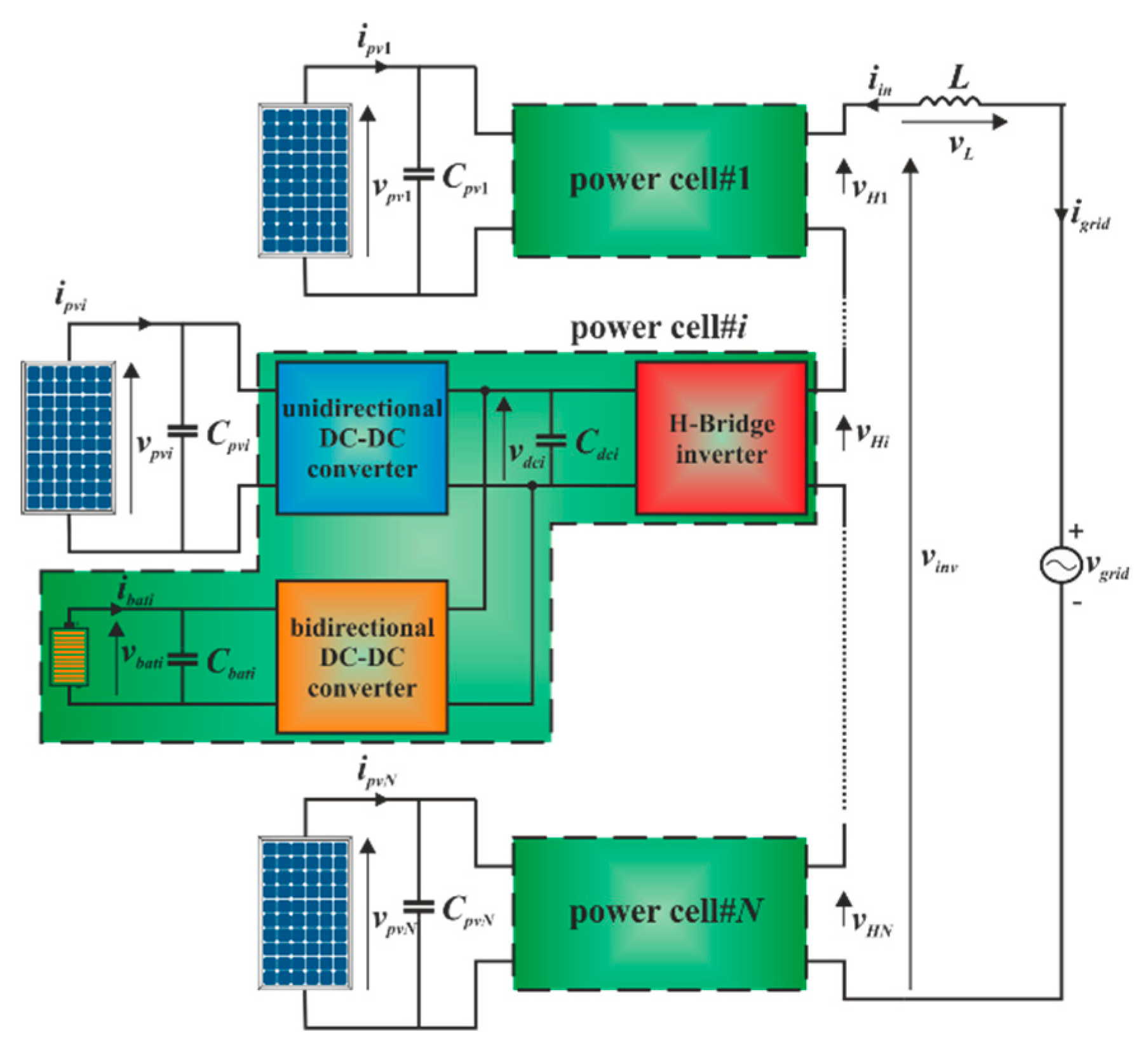
The architecture of distributed PV module-level CHB inverter is shown in
Figure 1. It consists of
N series-connected power cells forming a double stage dc/ac converter and a backup module consisting of a battery and a bidirectional dc-dc converter. A filter inductor
L connects the power cell output to the grid enabling the injection of sinusoidal current with a unity power factor (PF). As in the case of the multi-stage inverter, the power decoupling is achieved by means of a capacitor located in parallel to PV module (
Cpvi) and of dc-link capacitor (
Cdci), properly sized to guarantee a reduced voltage ripple at the rated power level. Then, a capacitive filter (
Cbati) is added in parallel to the battery. Finally, a single PV module supplies each power cell implementing a DPGS.
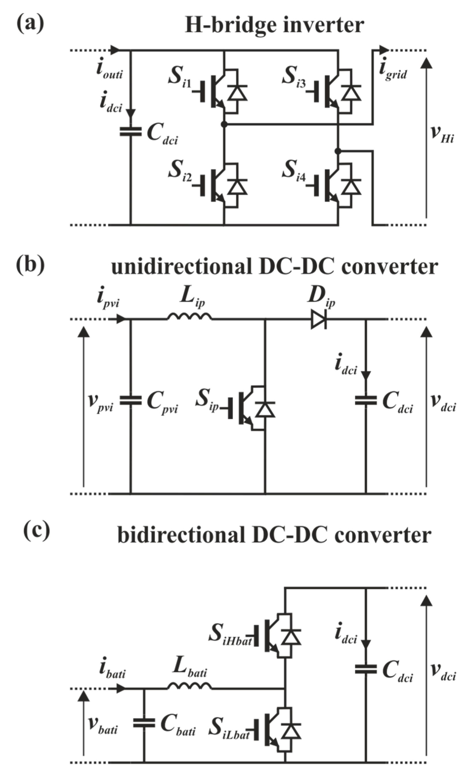
Figure 2 shows the schematic view of the power cell sub-circuits.
The main operation of the circuit can be described as follows. The overall inverter ac output voltage is
where
vHi is the output of
i-th power cell and can be easily expressed as
Si,j being the logic state of the
j-th switch in the
i-th cell (see
Figure 2a); the switch conducts when
Si,j = 1, while is off when
Si,j = 0. By considering
Si,1 =
i,2 and
Si,3 =
i,4, the control signal
hi can assume three discrete values: +1 (i.e.,
Si,1 = 1 and
Si,3 = 0), −1 (i.e.,
Si,1 = 0 and
Si,3 = 1), 0 (i.e.,
Si,1 =
Si,3).
By replacing
hi with a continuous switching function
si, the system dynamics can be modeled as follows:
The interface between each PV module and the corresponding dc-link is realized by means of a dc-dc boost converter, which is shown in
Figure 2b. It is a unidirectional converter which enables the power transfer from the PVG to the dc-link. Its main role is to ensure that the PV operation point is the one that maximizes the extraction of power or rather the maximum power point (MPP). In order to dynamically track the MPP, the value of the PV voltage reference is evaluated by an MPPT algorithm, independently performed for each PV module, thus allowing a DMPPT. The dc-dc boost converter is operated in Continuous Conduction Mode (CCM) by properly sizing the circuit parameters.
The interface between each battery module and the corresponding dc-link is realized by means of a buck-boost dc-dc converter, which allows us to control the bidirectional energy flow between the storage device and dc-link (see
Figure 2c). During the discharging operation mode, the power circuit acts like a boost converter and the power flows from the battery to the dc-link.
On the contrary, when the battery is charging, the power circuit behaves like a buck converter, whose input and output ports are represented by the dc-link and the battery terminals, respectively. It is worth noting that, in our case, the power to charge the battery is only provided by the PV module. In fact, the battery is devoted to mitigating the PV power fluctuations by absorbing the random excess of PV power w.r.t. power demand (i.e., BESS charging), while it can support the PV module when the extracted power is lower than the requested one (i.e., BESS discharging). As already discussed in the introduction, the former can avoid undesired curtailment of PV production, while the latter can assure continuous power supply, thus enhancing system reliability and flexibility. This translates into a flat output power profile regardless of the random variability of PV generation, so reducing the effect of intermittency of PVGs. In addition, as the results presented in the following bear out, it allows us to minimize the adverse impact of deep mismatch conditions.
3. Control Implementation
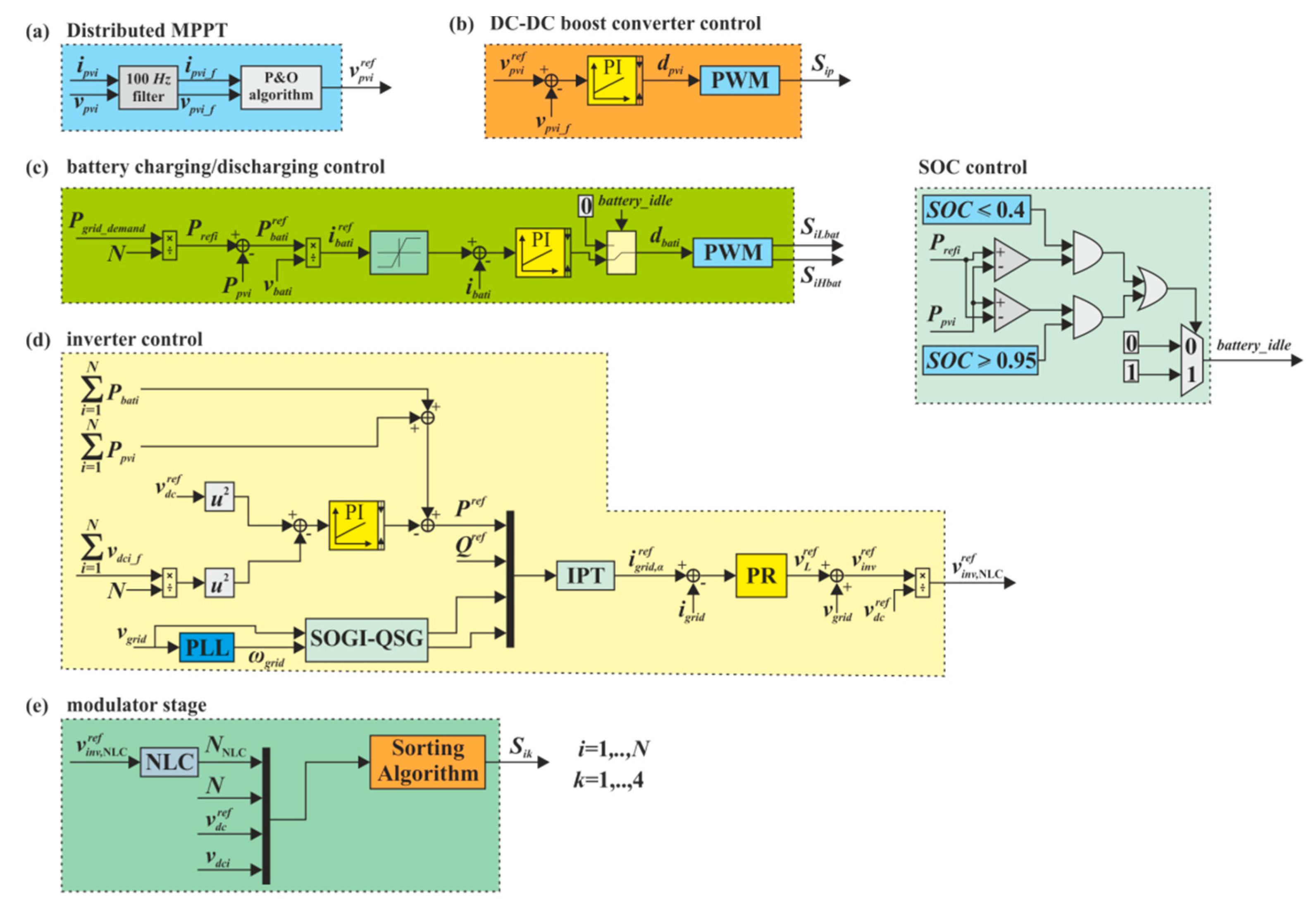
The proposed control scheme is shown in
Figure 3. It consists of five stages: the MPPT stage, dc-dc boost converter control, the charging/discharging control of the battery pack, the inverter control loop and the modulator stage. The first stage provides dedicated MPPT controllers, which perform individual MPP tracking of each PV module, based on the P&O algorithm, whose execution time interval is
TMPPT = 100 ms. Each MPPT section performs a fixed-step perturbation of the reference voltage
with a voltage reference step equal to
Δpv = 0.3 V. The input of the second stage is the PV voltage error, while the output is the duty cycle to proper control the dc-dc boost converter, so allowing to track the MPP of the corresponding PV module.
The third stage performs the charging/discharging of the BESS. The battery power reference
is the difference between the power demand,
Pgrid-demand (i.e., power requested by the grid) and the measured PV power,
Ppv. A positive
means that the battery will be in discharging mode thus supporting the PV generation to accomplish with the grid request. On the other hand, if
results to be negative, the battery can be charged by the excess of PV production w.r.t. power demand. As a consequence, the use of BESS reduces the impact of PV fluctuations and ensures a higher penetration of RES into the grid [
27]. The battery power reference is then divided by the measured battery voltage
vbat to obtain the desired battery current reference
, which is then properly limited to the maximum allowable value
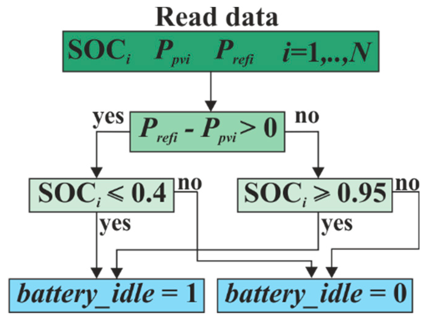
Ibat,max. The current error represents the input of a PI regulator, whose output is the duty cycle to drive the bidirectional dc-dc converter by means of PWM block. The battery idle control signal takes into account the battery condition. In fact, one more issue to be addressed is to preserve the health and stability of the battery so reducing possible fault conditions. For this purpose, an SOC (State of Charge) control is also implemented to avoid overcharge/discharge of the battery: if the SOC ≤ 0.4, the battery cannot be discharged, while if the SOC ≥ 0.95, the battery cannot be charged. In both cases, the battery goes in idle mode and it is disconnected from the dc-link by acting on the switching signals of the dc-dc converter. When the battery is in idle mode, the output power reference cannot be equal to the grid power demand, but it can be at the most equal to available PV power.
The fourth stage represents the inverter control loop, whose main goal is the transfer of the requested active power to the grid with unity power factor and low distortion. It consists of a dual-loop controller, where the outer control loop is based on the voltage-squared control method [
28] applied to the dc-link voltages. A PI controller provides the value of active power needed in order to cancel the error between the average of the
N measured dc-link voltages and the dc-link voltage reference
, which is the same for all the power cells to keep a balanced condition among the cells themselves [
29]. The inner control loop has the main task of controlling the grid current. The control strategy is based on the instantaneous power theory (IPT) [
30,
31], which operates with voltages and currents expressed in the stationary reference frame: the positive and negative sequence of the grid current are functions of the desired instantaneous active
and reactive power
, as follows
is the inverter current in the stationary reference frame. The voltage components
are grid voltages in a stationary reference frame. In a single-phase system, these two components can be emulated by a second order generalized integrator (SOGI), which may be considered a very suitable method for quadrature signal generation (QSG). It is worth highlighting that only the α component is controlled in single-phase system. Once the reference of the grid current positive-sequence is obtained, the grid current control is achieved by a proportional resonant (PR) controller. It presents a pair of poles on the imaginary axis at the frequency of the sinusoidal waveform (i.e., in our case the grid frequency), which it is desired to follow. Finally, the PR output provides the reference inductor voltage,
, which summed to the grid voltage, gives the inverter voltage reference,
. This latter quantity is then normalized w.r.t. the dc-link voltage reference and the result (
) becomes the input of the modulator stage, where an NLC (Nearest Level Control) achieves individual control of each power cell. The basic concept of the NLC is to approximate the reference of the output inverter voltage with the closest integer voltage level that can be generated by the CHB, referred to as
NNLC [
32,
33]. Hence,
NNLC can only assume integer values in the range (−
N, +
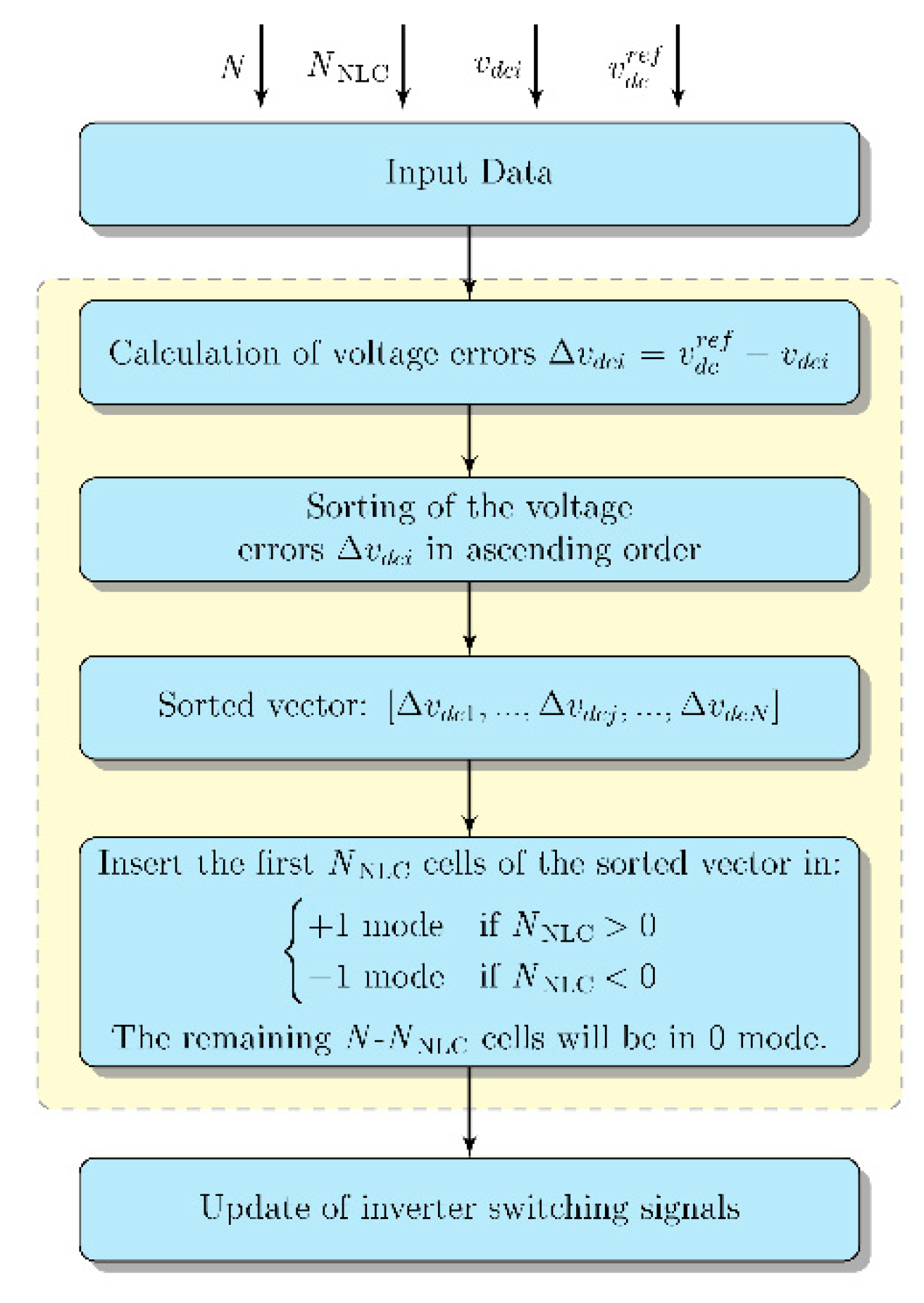
N). In particular, the adopted NLC control is based on a sorting algorithm (see
Figure 4) taking the decision of which power cell will be inserted (±1 mode) or bypassed (0 mode) at every time step,
Tsort. At the starting point, the voltage error at each dc-link as the difference between dc-link voltage reference and the filtered measured dc-link voltage is calculated. Then, the choice of cell operating mode is made by considering the need to charge or discharge the cell itself (i.e., the dc-link capacitor) in order to track the desired voltage reference
. As a consequence, a positive error implies that the cell dc-link must be charged and the consequent action is to bypass the cell (i.e., 0 mode), so allowing the PVG to charge the corresponding dc-link, meanwhile, the cell output voltage
vHi is zero. On the contrary, a negative error calls for discharging the cell dc-link to follow the desired reference and the consequent action is to insert the cell (i.e., ±1 mode), while the cell output voltage is equal to ±
vdci (the sign depends on the detected sign of
NNLC). The procedure is described in the flow chart of
Figure 4. The
N dc-link voltages are sorted in ascending order, so the first position (i.e., #1) is associated with the power cell with the lowest negative error, while the last position (#
N) is associated to the cell with the highest positive error. To properly synthesize the inverter multilevel waveform, the first
NNLC power cells of the sorted vector will be kept in discharging mode (±1 mode), while the remaining
N-
NNLC cells will be bypassed (0 mode corresponding to the charging mode). The switching signals do not change until the next execution of the sorting algorithm, with a time step equal to
Tsort = 1 ms.
4. Simulated Performance
A set of simulations has been performed on 19-level PV CHB inverter (i.e., N = 9) with integrated BESS in the PLECS environment. In order to reduce the computational load, the average model of the power circuits has been used. This latter choice does not affect the obtained results in order to prove the feasibility and effectiveness of the proposed design and control strategy. It is worth noting that the cell number can be chosen by firstly considering the ac-side requirements. In fact, the maximum inverter voltage must allow us to inject into the grid the active nominal power. If a unity power factor is considered, the amplitude of the inverter voltage depends on the line inductance L and on the desired output power. In the considered case (i.e., L = 10 mH, and a nominal power of 1.8 kW), the peak inverter voltage reaches 327 V. The overall dc-link voltage of the cascade structure (i.e., the sum of the dc-link voltages of the individual cells) must be greater than the peak to properly synthesize the multilevel inverter output voltage, thus defining the minimum needed number of cells in the cascade structure. Note that the dc-link voltage of the individual H-bridge cells is chosen to be greater than the open-circuit voltage of the PV modules to ensure the boost operation of the dedicated dc-dc converter performing the MPPT. In our case, the dc-link voltage reference was set to 48 V, thus resulting in minimum number of cells of 7. Finally, the number of cells was increased to 9 to ensure the redundancy useful to also provide a fault-tolerant capability.
At the input of each power cell, the PV generators [
34] are described in simulation through a physical model based on a generalization of the five parameters single diode model. The current source
iph accounts for the photogenerated current, the ideal diode (i.e., resistive free) accounts for the dark I-V characteristic, it is fully defined by the reverse saturation current
Isat and the ideality factor
n.
Rs and
Rsh are the series and shunt resistance, respectively, accounting for parasitic effects. In order to describe an arbitrary number of solar cells series-connected, due to a solar module under uniform standard operating conditions, it is well-known and widely accepted a generalization of the previous model. The I-V characteristic of an arbitrary string is described by equation
where
vpv is the voltage across a PV module, composed of
n1 solar cells.
VT is the junction thermal voltage,
Rs,
Rsh,
iph,
Isat and
n are the five parameters of the single diode model. The values adopted for the model parameters are reported in
Table 1. The operating point at STC results in
PMPP = 331.55 W corresponding to
VMPP = 37.6 V and
IMPP = 8.82 A at STC.
Moreover, the most meaningful parameter to look at, in order to find the proper size of the battery pack, is the capacity of the battery. However, for the sake of a simple modeling, the battery capacity is assumed to be constant even under variable discharging current rates. It is now worth pointing out the definition of other parameters of interest: the state of charge and the energy stored.
The State of Charge (SOC) is a measure of the residual capacity of the battery. It is defined in Equation (6), where Q0 is the total charge that the battery can store and ib is the discharging current.
In addition, it is well known that realizing a reliable battery model is difficult, due to the dependency of the battery performance on several parameters, some of which are really hard to specify. Nevertheless, a simplified model, well-suited for our purposes, has been implemented for the simulation. The equivalent circuit of the battery consists of an ideal voltage source, which provides the open-circuit voltage Voc, in series with a constant internal resistance Rint. In general, both the voltage source and the resistance are affected by the SOC and the temperature. For the sake of simplicity, only the dependency of the open-circuit voltage on the SOC will be taken into account.
The effective relationship between
Voc and SOC depends on the chemistry of the battery and it is usually provided by the manufacturers by means of the discharging curves. However, the non-linear pattern between
Voc and SOC can be qualitatively yielded as
where
E0 is the standard potential of the battery,
R is the ideal gas constant,
T is the absolute temperature and
F is the Faraday constant. The SOC control, already presented in
Section 3, is now better highlighted by means of a proper flowchart reported in
Figure 5. The battery sizing derives from the need to support the PV power generation to accomplish with the grid demand. As a consequence, it has been considered a storage unit able to provide the PV module peak power (i.e., 331.55 W at STC) for half an hour corresponding to a battery energy of about 165 Wh. This choice relies on the possibility of mitigating a short term variability of PV production due to change in irradiance or temperature and shadowing phenomena. So, the used battery pack presents a capacity of 5 Ah, with a rated voltage of about 36 V and the total internal resistance of 30 mΩ.
To verify the performance of the proposed system, two different scenarios were considered: uniform and mismatch static conditions. In addition, the analysis was also conducted on the same circuit architecture with no battery with the aim of demonstrating the enhanced performance due to the presence of the distributed storage system.
The grid demand was set, in all considered cases, to 1.8 kW corresponding to a power reference for each cell equal to
Prefi = 1.8/9 = 200 W, thus the different results were obtained with the same output power in order to make a fair comparison. The dc-link voltage reference of each power cell is fixed to
. The initial SOC of each battery pack is set to 50%, while its minimum and maximum limits are 40% and 95%, respectively (see also
Figure 3).
4.1. Static Uniform Conditions with Battery
In the first experiment, to emulate PV sources under uniform irradiance conditions, the nine PV models were set at the same irradiance level of 1000 W/m
2, corresponding to a
PMPP = 331.55 W, and the steady-state behavior of the system was considered. In such a case, the difference between the PV available power and the requested one (i.e.,
PMPP −
Prefi ≈ 131 W) is used to charge the battery.
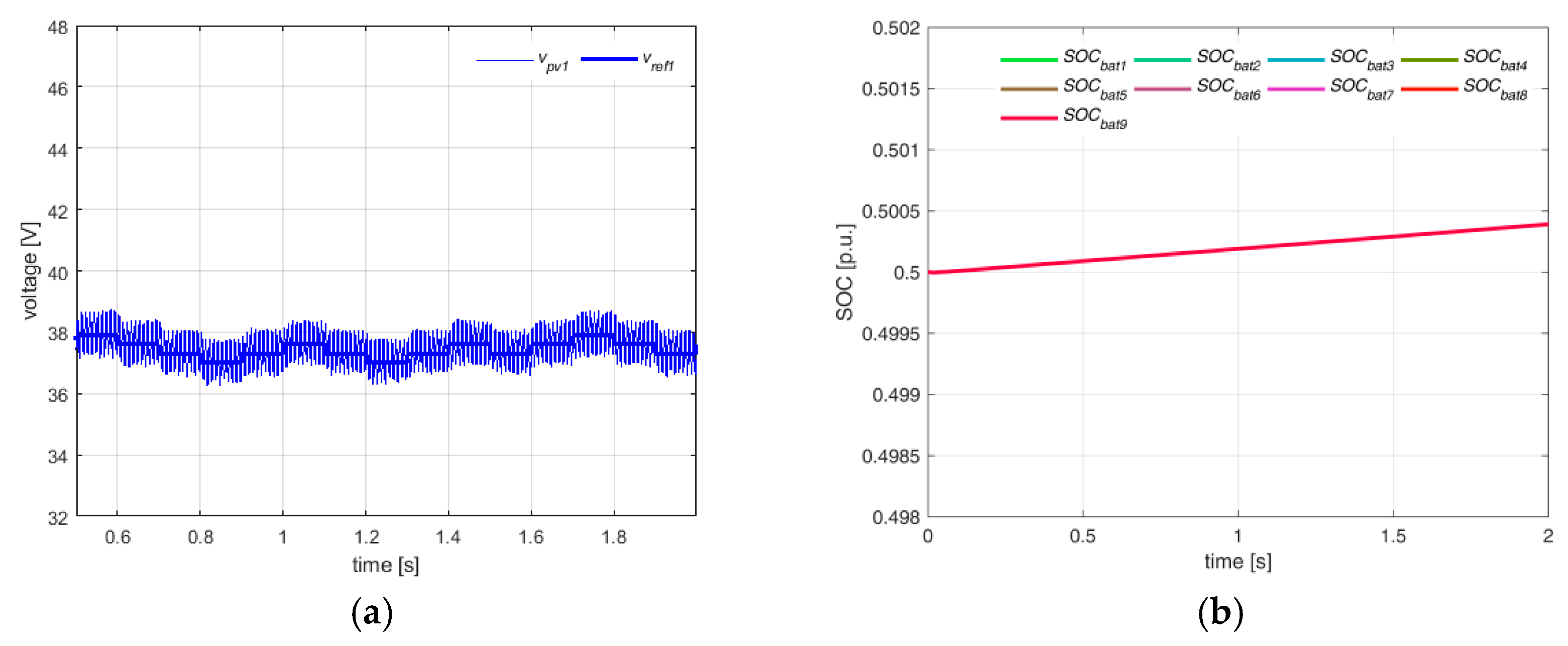
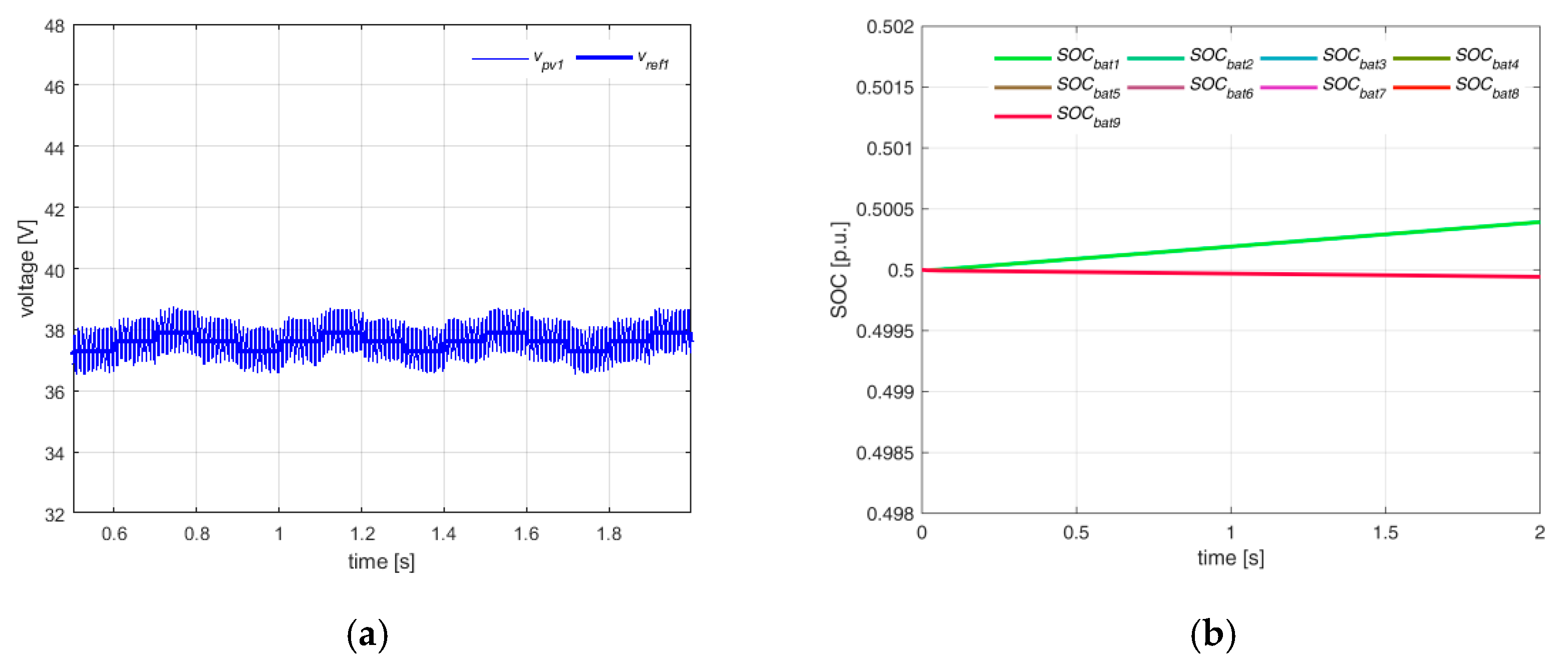
Figure 6a) shows, as an example, the tracking behavior of the first power cell. The overall MPPT efficiency is greater than 99%, because, as expected in uniform condition, each cell operates close to the MPP voltage of 37.6 V, while
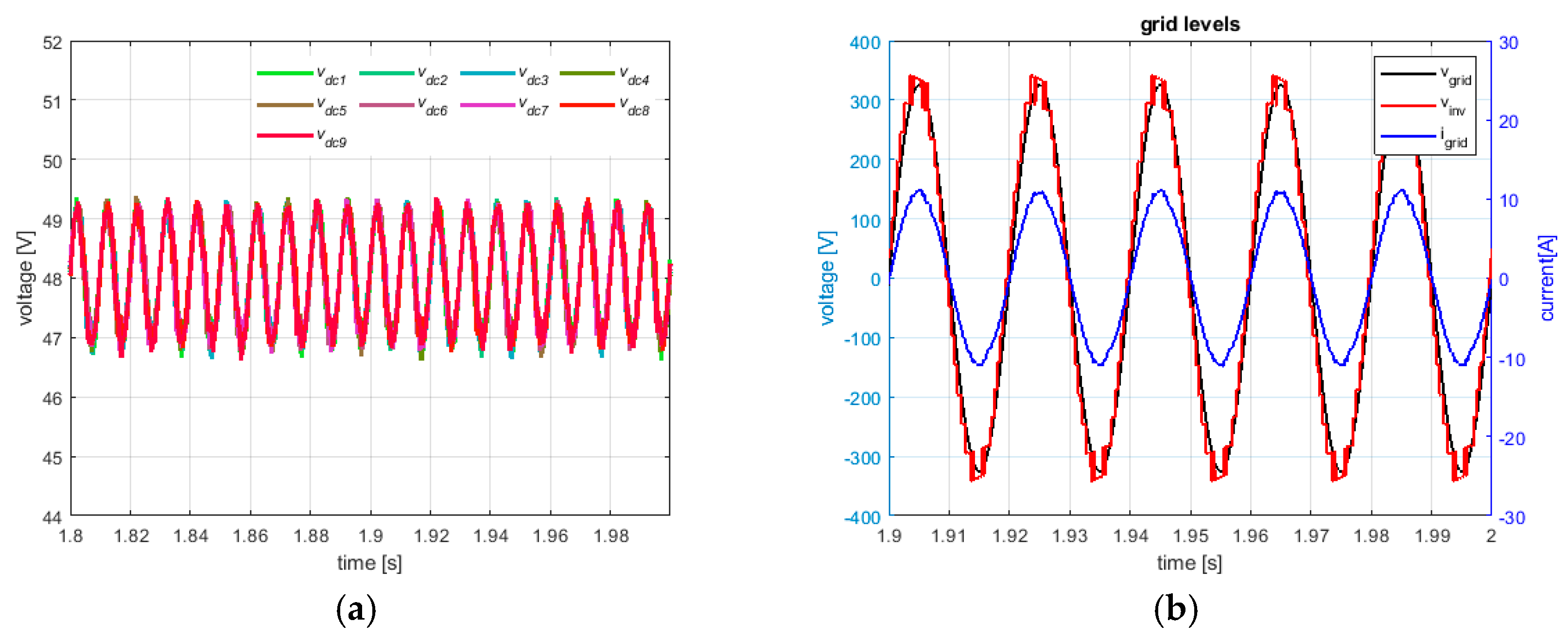
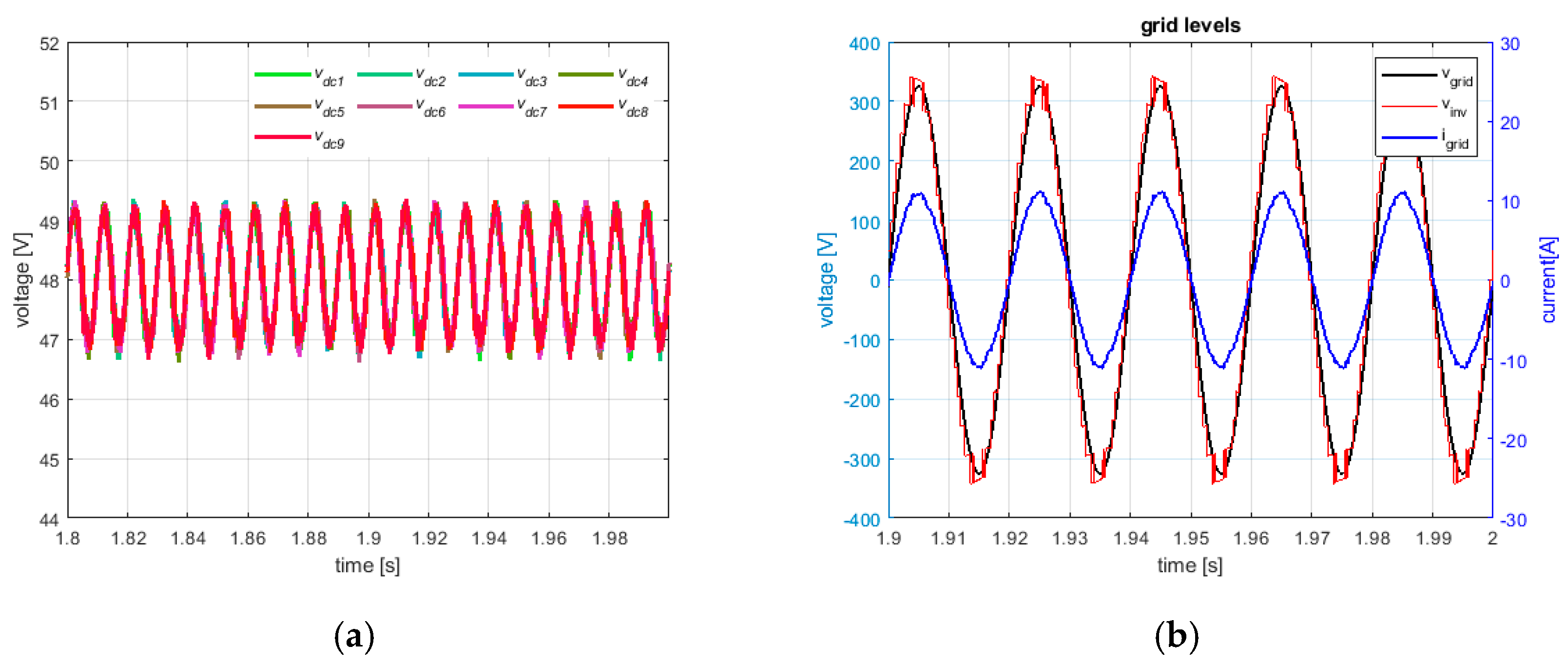
Figure 6b) shows the SOC increasing of each cell. The steady-behavior at the dc-link is reported in
Figure 7a, where it can be seen that the dc voltages properly track the voltage reference of 48 V. At ac side, the grid current results sinusoidal in phase with the grid voltage (see
Figure 7b), thus leading to an almost unity power factor and a low value of THD (i.e., about 2.4%). This latter quantity was calculated on the first 40 harmonics.
4.2. Static Uniform Conditions without Battery
In such a case, to simulate the system in the same conditions of the previous one, the nine PV models were set at the same irradiance level of 603.31 W/m
2, corresponding to a
PMPP = 200 W, thus resulting in the same output power of 1.8 kW.
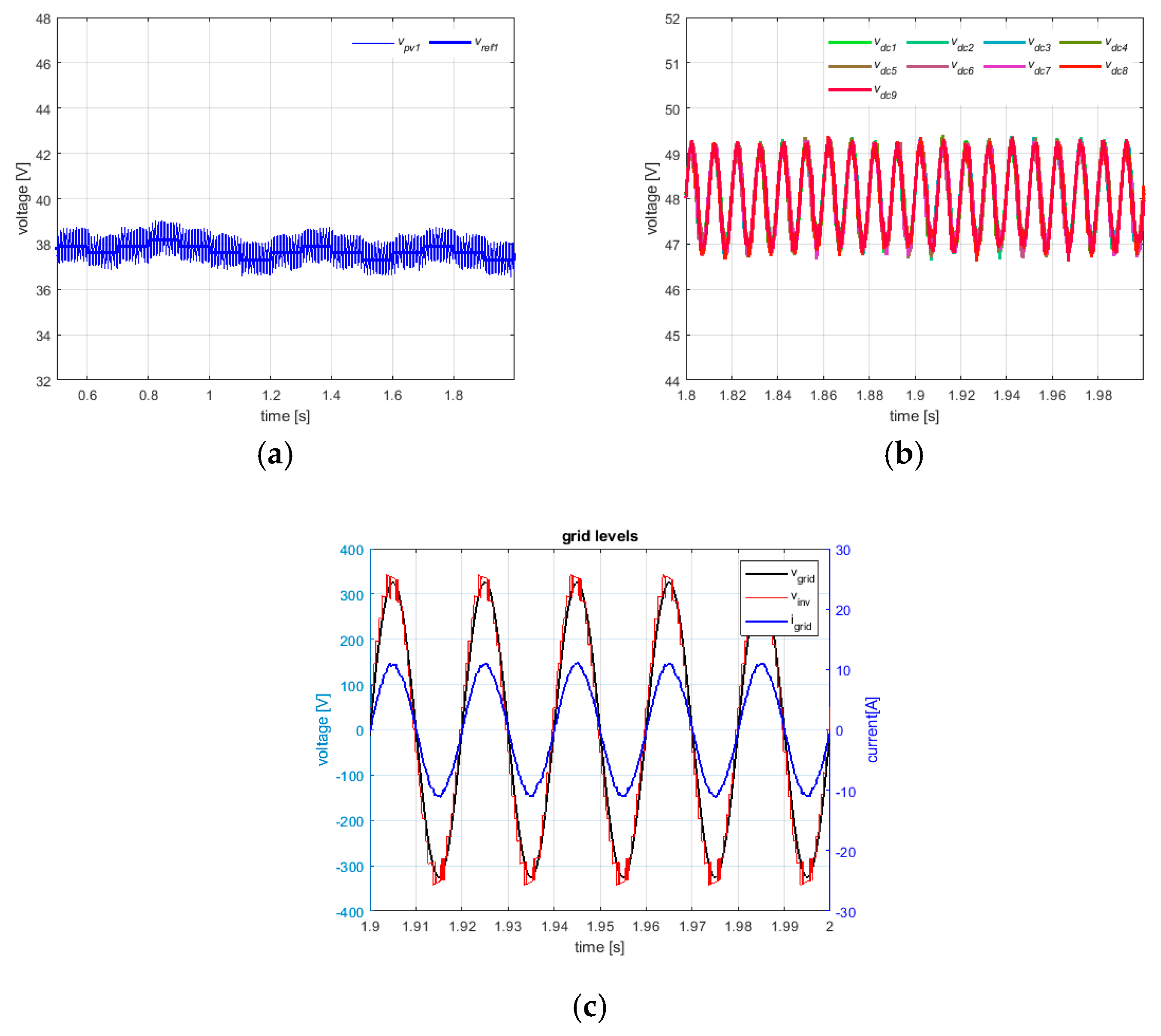
Figure 8a) shows the tracking behavior of the first power cell. Obviously, also, in this case, the overall MPPT efficiency is good and greater than 99%, because, as expected in uniform condition, each cell operates close to the MPP voltage.
The steady-behavior at the dc-link is reported in
Figure 8b, where it can be seen that the dc voltages properly track the voltage reference of 48 V. At ac side, the grid current results sinusoidal in phase with the grid voltage (see
Figure 8c), thus leading to an almost unity power factor and a low value of THD (i.e., about 2.4%).
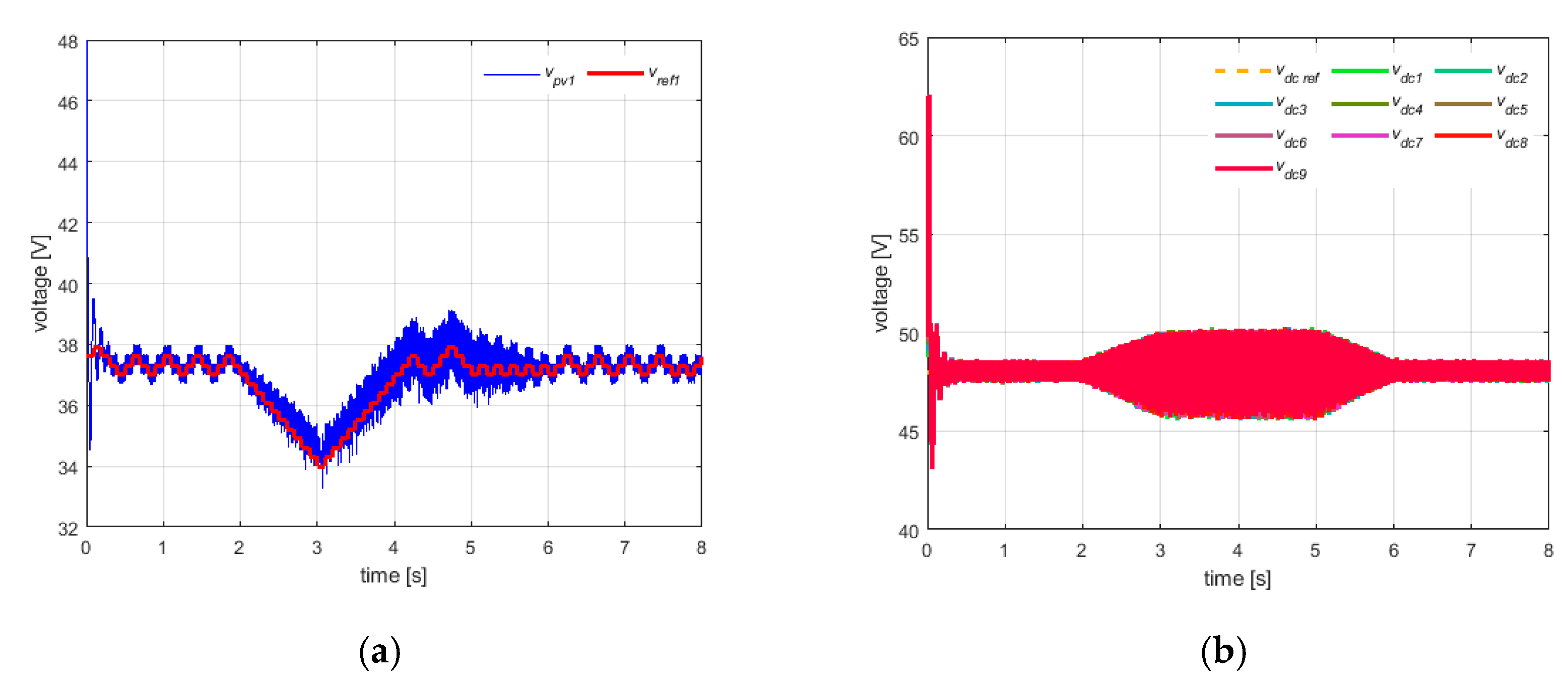
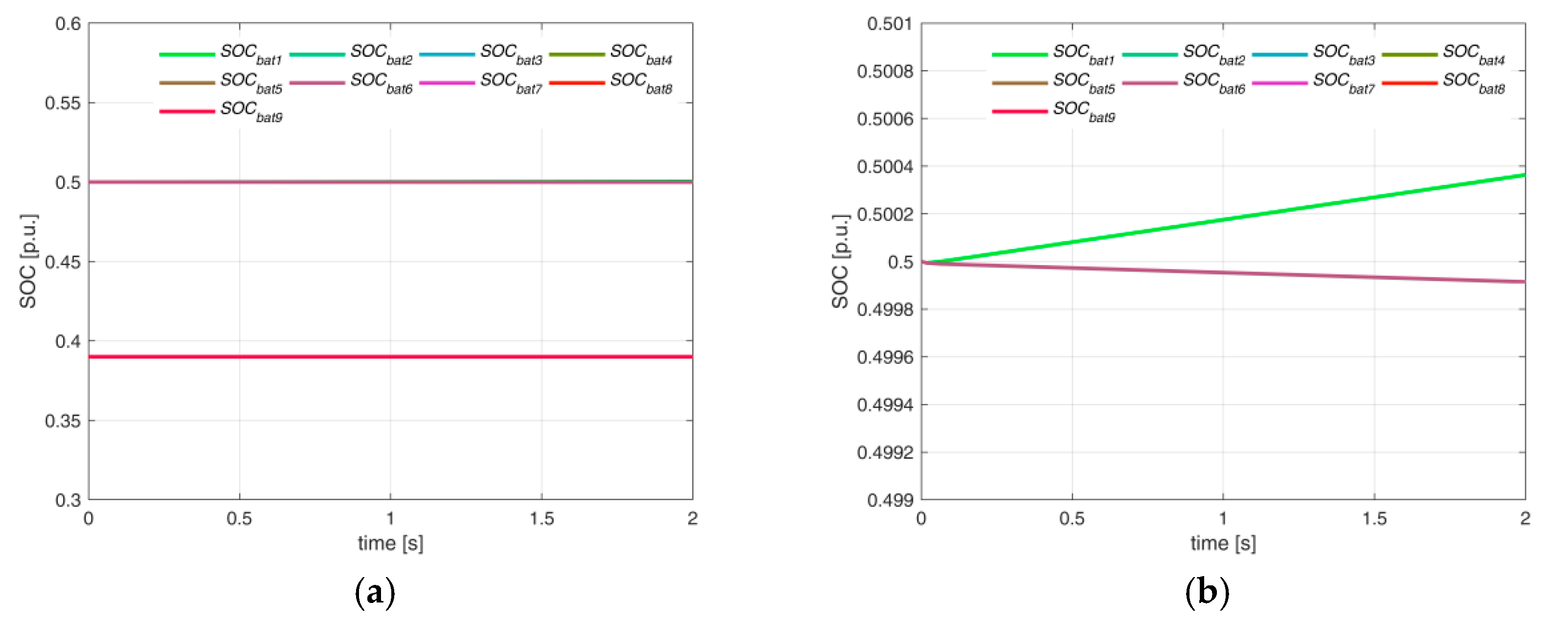
4.3. Mismatch Conditions with Battery
The second simulation provided information about system behavior under mismatch conditions. The effect of mismatch among PVGs on the dc-link voltages was investigated.
The tests were performed under the irradiance conditions, obtained by supplying the first power cell with 1000 W/m2 (i.e., 331.55 W), and the remaining 8 cells with 554 W/m2 (i.e., 183.6 W). In such a case, for the first cell, the difference between the PV available power and the requested one (i.e., PMPP − Prefi ≈ 131 W) is used to charge the battery, while for the remaining 8 cells the negative power balance PMPP − Prefi ≈ −16.5 W is provided by the batteries.
Figure 9a shows the tracking behavior of the first power cell. As can be seen, the mismatch conditions among the PVGs does not affect the overall MPPT efficiency which is greater than 99%, because, as expected, each cell operates close to the MPP voltage thanks to the front-end dc-dc converter, which allows independent MPPT.
Figure 9b shows the SOC behavior and, as expected, it increases for the first cell (green line in
Figure 9b), which is in charging mode, while decreases for the other cells, which are in discharging mode (red line in
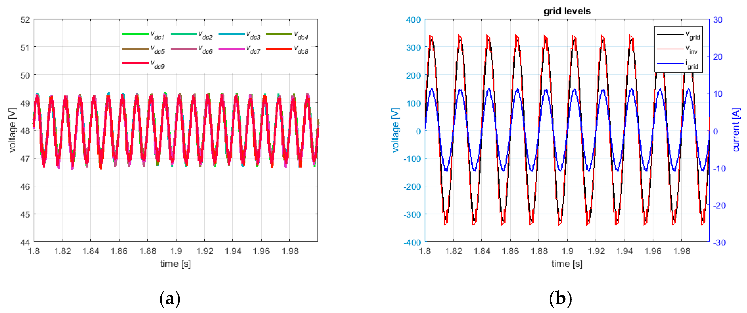
Figure 9b). As a consequence, the BESS is able to cancel the effects of PV power fluctuations by obtaining a flat profile of the output power, which meets with the power demand, thanks to a balanced power-sharing at each dc-link, whose voltages again properly track the voltage reference of 48 V (see
Figure 10a).
At the ac side, the grid current results sinusoidal in phase with the grid voltage (see
Figure 10b), thus leading to an almost unity power factor, and THD of about 2.4%.
4.4. Mismatch Conditions without Battery
In such a case, to simulate the system in the same conditions of the previous one, or rather with the same output power, the PV models were set at the same manner by supplying the first power cell with 1000 W/m2 (i.e., 331.55 W), and the remaining 8 cells with 554 W/m2 (i.e., 183.6 W). The overall output power is about 1.8 kW corresponding to the power request.
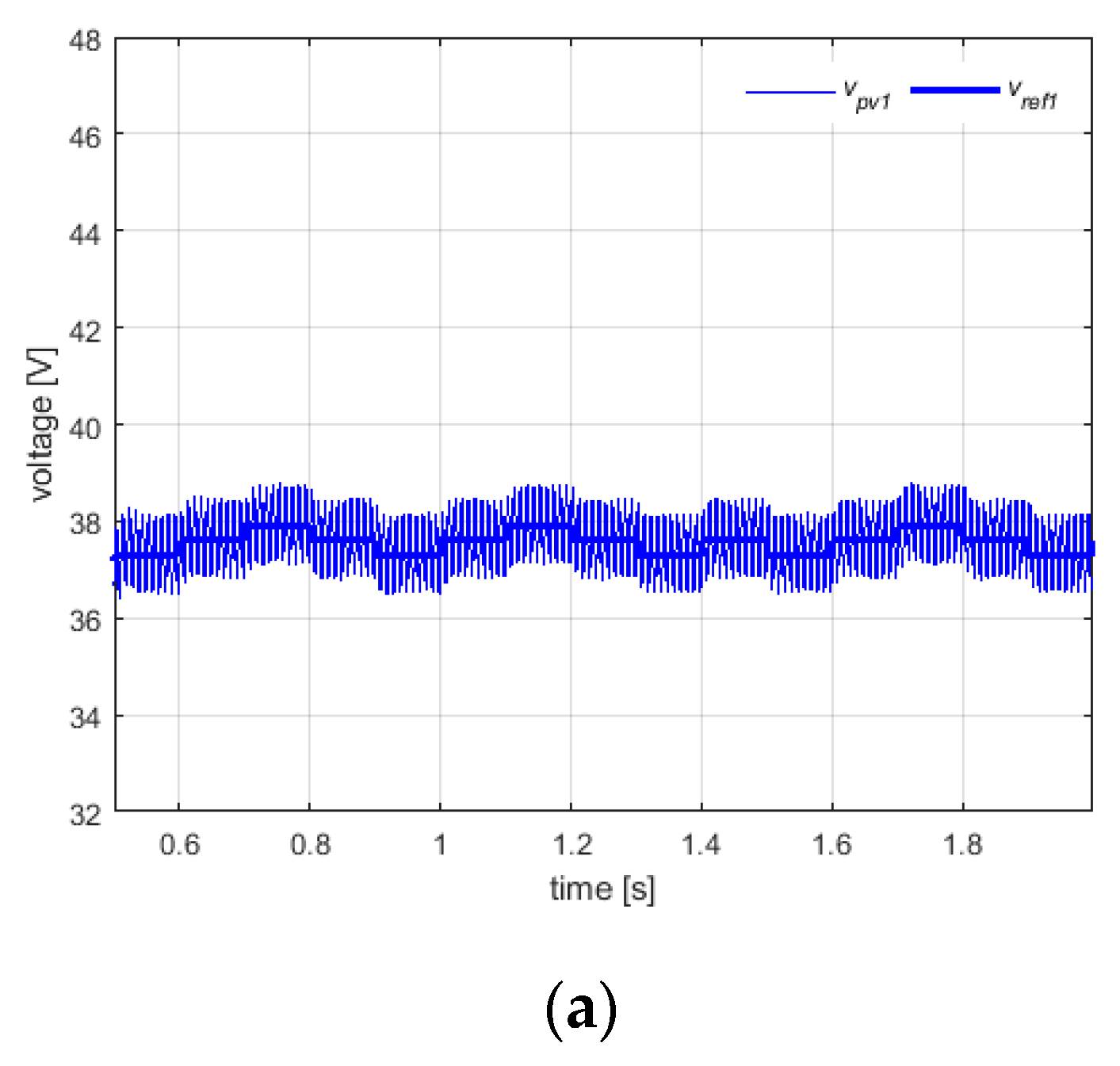
Figure 11a shows the tracking behavior of the first power cell. As can be seen, the mismatch conditions among the PVGs does not affect the overall MPPT efficiency which is greater than 99%, because, as expected, each cell operates close to the MPP voltage thanks to the front-end dc-dc converter which allows independent MPPT. The steady-behavior at the dc-link is reported in
Figure 11b, where it can be seen that the dc voltages properly track the voltage reference of 48 V in the case of the lower power cells (i.e., the 8 cells supplied by the PV panels at 554 W/m
2), while the most powerful cell (i.e., the first cell with PV panel at 1000 W/m
2) deviates from the dc-link voltage reference or rather the system continues to operate but this cell is no more able to track the reference.
In fact, in the circuit topology without battery it is not possible to reach a balanced power-sharing at each dc-link, thus, by considering that the power cells share the same output current (due to the series connection) the higher power cell should adapt itself by handling its own power at a higher voltage level (i.e., reduced current). What happens is that the higher power level cannot be handled by the cell itself, thus any power excess is transferred to the dc-link capacitor, whose voltage increases, so determining a difference between the dc-link voltage reference and the actual dc-link voltage. Obviously, this means that the cell can no longer track the dc-link reference, thus leading to a lack of control action. Practically, the system operation under mismatch conditions can cause high-power cells to reach the overmodulation region.
It is clear, from the previous discussion, that the role of the battery is crucial to avoid a deviation of the dc-link voltage of the more powerful cell from its reference which translates in a lack of balancing control. In the PV CHB architecture, this result can be only obtained by means of a distributes BESS, where each power cell is equipped with its own backup module. In fact, a central battery could only be connected at the ac side, thereby losing the possibility of compensating the effect of a mismatch for each individual power cell.
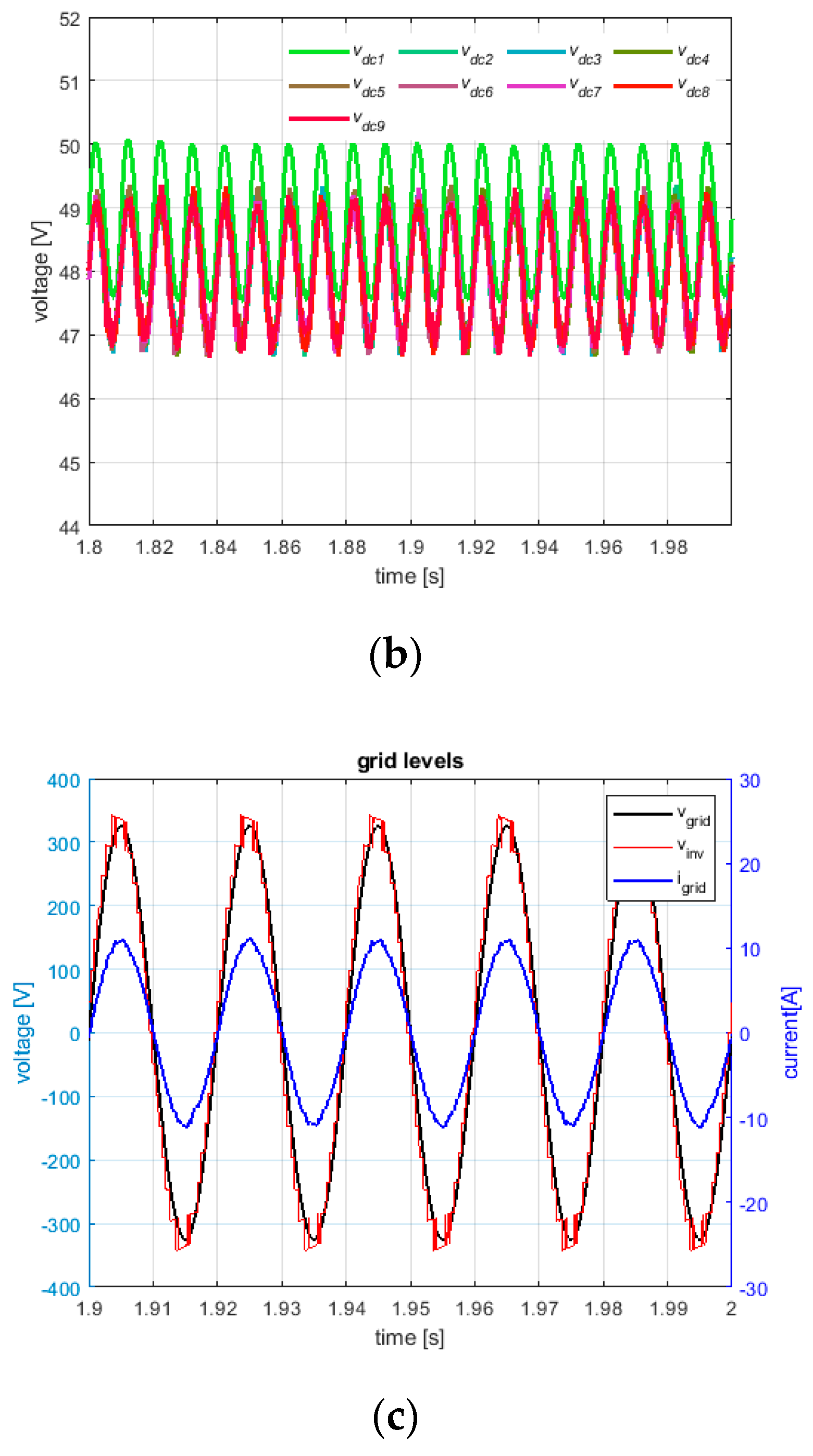
Finally, the grid current results to be sinusoidal and in phase the grid voltage (see
Figure 11c), thus leading to an almost unity power factor, and a THD of about 2.4%.
4.5. Dynamic Uniform Conditions with Battery
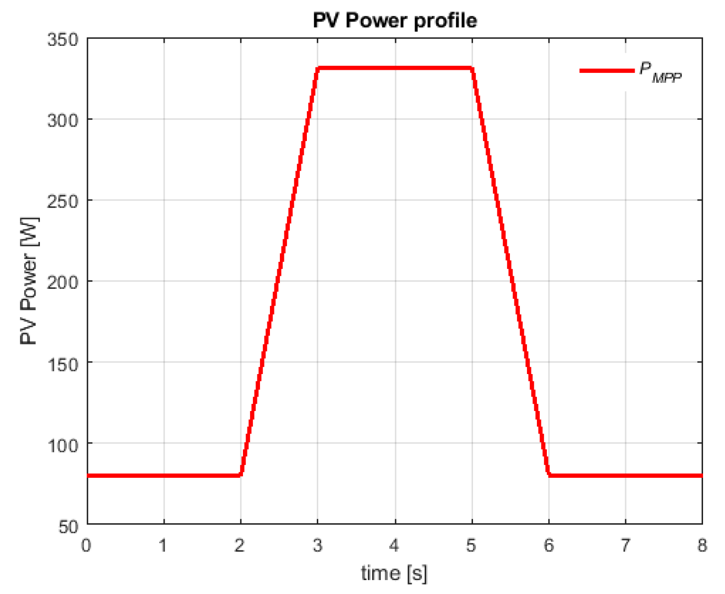
The last analysis was performed to investigate the behavior of the system under dynamic uniform conditions corresponding to a cloudy-sky. During the simulation, the system is dynamically forced to move from a uniform condition at low irradiance (i.e., 250 W/m2 corresponding to an MPP power of 82.89 W) to a higher irradiance at STC (i.e., 1000 W/m2 corresponding to an MPP power of 331.55 W).
The PV model of each power cell tracks a dynamic irradiance profile whose corresponding PV power is depicted in
Figure 12 (i.e., the PV power cycle).
As it is shown, the irradiance value switches between 250 W/m2 and 1000 W/m2 with a dwell time of 2 s and rise/fall time of 1 s. The overall requested power is always fixed to 1.8 kW (corresponding to 200 W per power cell).
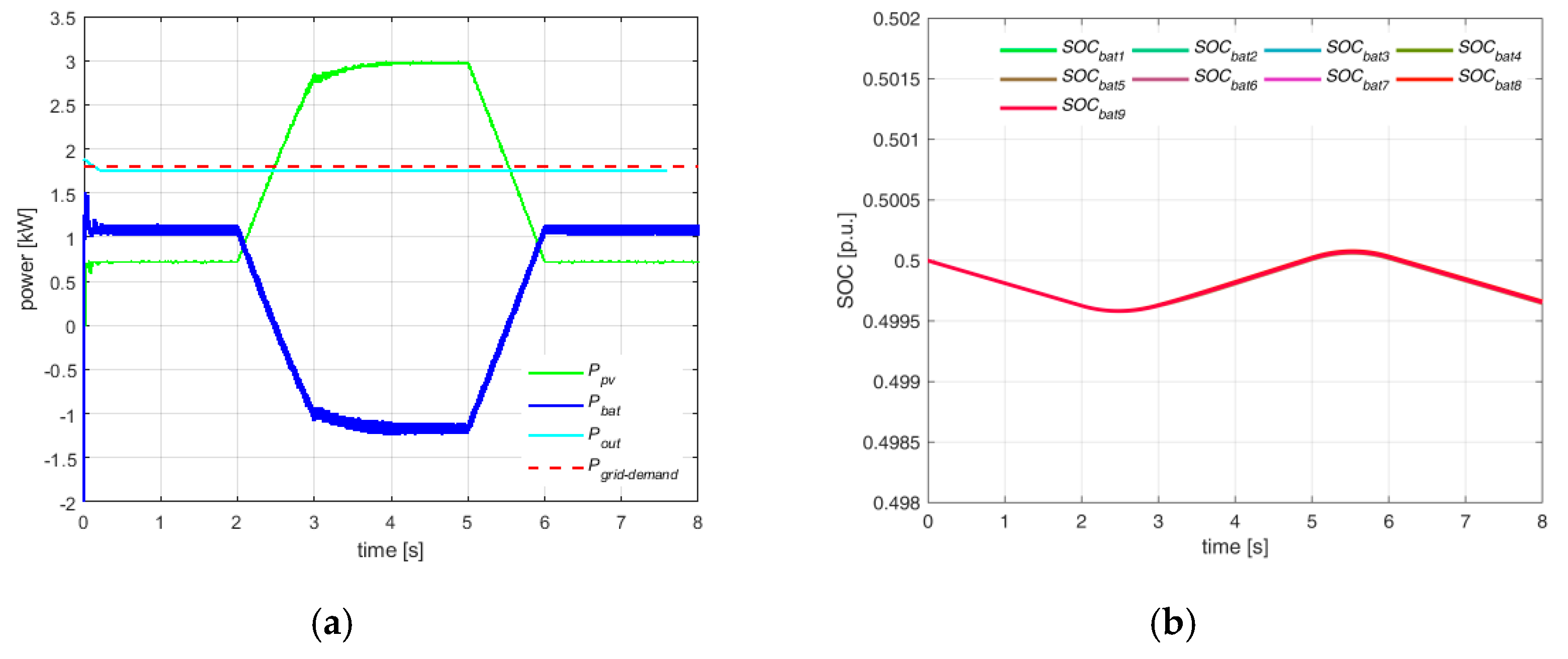
This dynamic test is useful to demonstrate that, despite PV power variability, the output power profile remains flat thanks to the presence of the storage unit which is able to compensate for the PV power fluctuations by absorbing the random excess of PV power w.r.t. on-time demand (i.e., BESS charging), while it can support the PV module when the extracted power is lower than the requested one (i.e., BESS discharging).
Figure 13a shows the power behavior during the test cycle of
Figure 12. It can be noted that PV power varies, due to different irradiance levels, and the battery power correspondingly varies, thus mitigating the effect of PV power randomness and obtaining a flat profile of the power transferred to the grid also properly meeting the grid demand.
Figure 13b also reports the time behavior of batteries SOC.
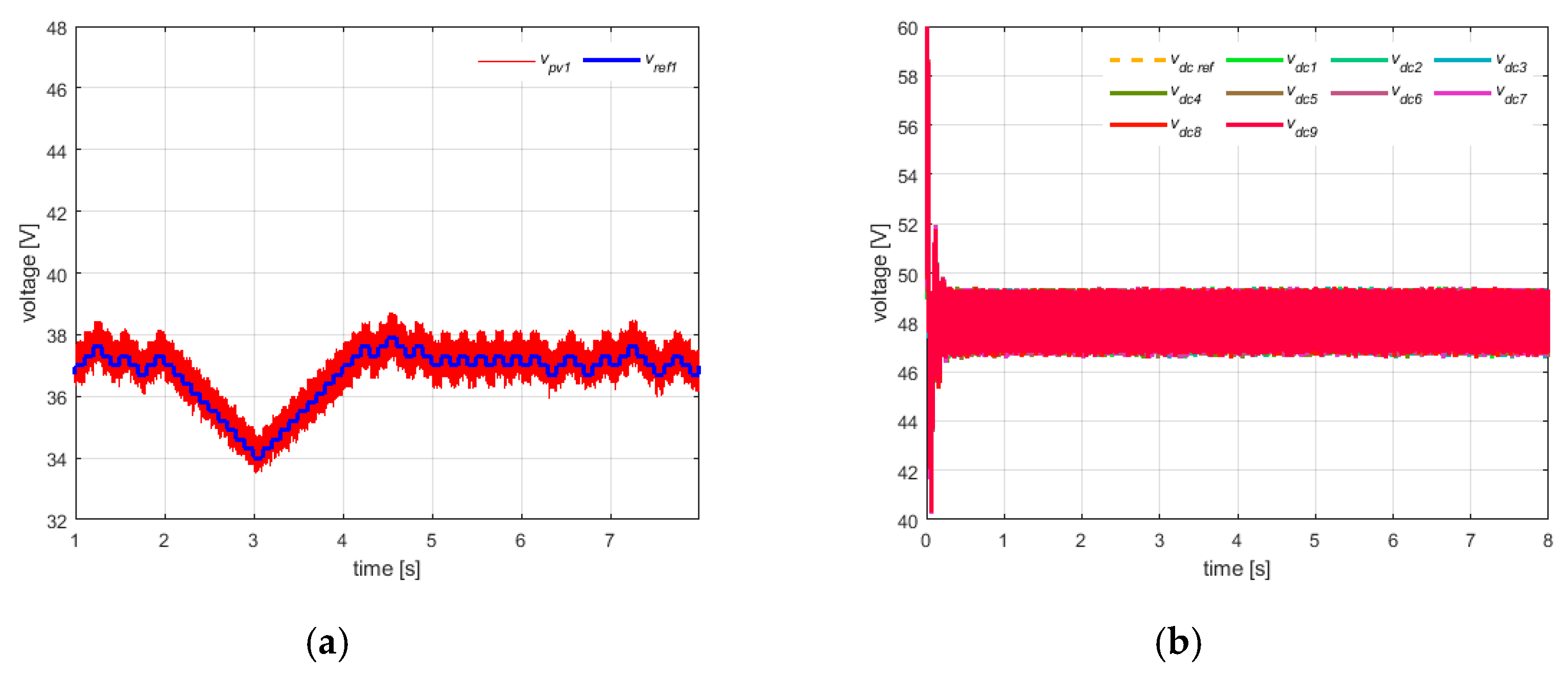
Furthermore,
Figure 14a shows the tracking behavior of the first cell which operates close to the MPP voltage, while
Figure 14b reports the behavior at the dc-link. It can be seen that the dc voltages properly track the voltage reference of 48 V also in dynamic conditions.
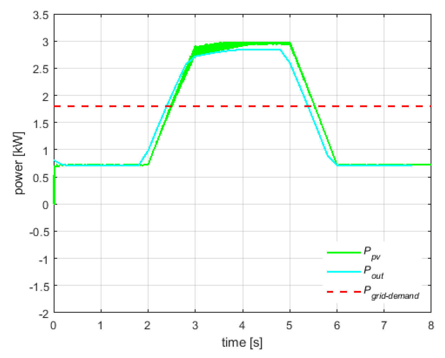
4.6. Dynamic Uniform Conditions without Battery
The same irradiance profile (i.e., PV power profile of
Figure 12) of the previous analysis is used also in this case in order to demonstrate that the absence of the battery does not allow to obtain a flat profile of the output power. As can be seen in
Figure 15, the output power follows the fluctuations of the PV power, thus it cannot meeting the grid demand. Moreover, also the tracking behavior of the MPP and of the dc-link voltage reference is adversely affected as shown in
Figure 16. In particular, the dc-link voltages result modulated by the PV power.
4.7. Case of Study: Static Mismatch Conditions with About 30% of Batteries Down
The test was performed under the same irradiance conditions of
Section 4.3, obtained by supplying the first power cell with 1000 W/m
2 (i.e., 331.55 W), and the remaining 8 cells with 554 W/m
2 (i.e., 183.6 W). As discussed
Section 4.3, during normal operation, in the first cell the difference between the PV available power and the requested one (i.e.,
PMPP −
Prefi ≈ 131 W) is used to charge the battery, while in the remaining 8 cells the negative power balance
PMPP −
Prefi ≈ −16.5 W is provided by the batteries. On the contrary, in the case of the study, the initial battery SOC of 3 of the 8 remaining power cells (specifically cell#7,8,9) is set to 0.39, which is lower than the minimum limit of 0.4. This latter means that these batteries cannot be further discharged, thus they cannot provide the negative power balance of
PMPP −
Prefi ≈ −16.5 W. In such a case, not only the PV production of these power cells results lower than the individual power request (i.e.,
Prefi), but also its own battery pack is not able to support this request (i.e., the battery is down or rather its SOC is lower than 40%). Generally, as already explained in
Section 3, when the battery is in idle mode, the output power reference cannot be equal to the power demand, but it can be at the most equal to available PV power. Nevertheless, the total power difference (i.e., 3 × 16.5 W = 49.5 W) could be evenly distributed among the power cells which have an overall power content (i.e.,
Ppvi +
Pbati) higher than the individual power request
Prefi. In this way, the system will be still able to meet the total power demand, so again resulting in a flat profile of the power transferred to the grid.
Obviously, this particular condition should be carefully taken into account by properly modifying the calculation of the individual power request (i.e., the power reference of each power cell,
Prefi) by considering if the corresponding battery SOC lies in the allowed range or not (i.e., the battery is in idle mode). As a consequence, the power reference of each power cell will be as follows
where
n (
battery_idle = 1) is the number of power cells with the battery in idle mode, while
Ppvi (
battery_idle = 1) is the corresponding
i-th PV power of the aforementioned cells.
Figure 17 shows the time behavior of the batteries’ SOC.
In particular,
Figure 17a shows that the battery SOC of the three cells in idle mode is constant and equal to its initial value of 0.39, while
Figure 17b highlights that the battery of the first cell is in charging mode (green line in
Figure 17b), while the batteries of the remaining five cells (i.e., cell#2, 3, 4, 5, 6) are in discharging mode.
Moreover, the dc-link voltages again properly track the voltage reference of 48 V as shown in
Figure 18a, while at ac side, the grid current results sinusoidal in phase with the grid voltage (see
Figure 18b), thus leading to an almost unity power factor and THD of about 2.4%. It is worth noting that if the mismatch of available power from each cell increases, due to battery absence (i.e., the battery in idle mode), the system will be able to properly meet the power demand until a condition of deep mismatch which cannot more suitably be handled without battery support. Nevertheless, it is worth highlighting that each battery pack is designed for a short term variability of PV generation profile to mitigate the PV power fluctuations in a timescale up to tens of minutes. As a consequence, it is possible to consider, on-time average, the batteries’ SOC will be likely within the allowed range.

 ,
, 


