1. Introduction
In the European Union (EU), buildings account for 40% of energy consumption and 36% of CO2 emissions. Directive 2010/31/UE establishes that member states draw up national plans to improve the energy efficiency of existing buildings and increase the number of new buildings with improved energy performance (nearly zero-energy buildings). This makes it even more important to characterize the building envelope, so that high-quality constructive details will be chosen.
The thermal behavior of the building envelope relies as much on the features of each building element (wall, roof, floor, door, and window) as it does on the two-dimensional (2D) and three-dimensional (3D) junctions of these elements, respectively referred to as linear thermal bridges (LTBs) and point thermal bridges (PTBs).
A thermal bridge increases the heat loss of a building envelope in winter conditions, due to a concentration of the heat fluxes that depends on the material properties and on its geometrical characteristics [
1,
2]. Some studies showed that the increased energy needs, due to the thermal bridges, are usually considerable and can be over 20% [
3]. Double-brick construction, used widely in many Mediterranean countries, is particularly susceptible to allowing the formation of thermal bridges. The application of insulation in the air cavity between brick panes is interrupted by the concrete structure. Furthermore, even if there is a thermal correction of those zones, insulation discontinuities often occur. In some cases, the thermal losses increase with high insulation levels.
Furthermore, the surface temperatures in thermal bridge details are normally significantly lower, which increases the risk of occurrence of building pathologies caused by surface condensations [
4,
5,
6,
7]. Therefore, it is of the utmost importance to evaluate the LTBs and PTBs at the design stage of the building and assess their influence on the energy consumed [
8].
Some authors have stated that the thermal behavior of thermal bridges should be predicted dynamically, assuming that temperature will change over time. The influence of the thermal inertia of materials is therefore taken into account [
9,
10,
11,
12]. On the other hand, in a steady state (static) analysis, the heat fluxes are assumed to be constant throughout the construction elements and thus the temperatures do not change over time. In an unsteady state (dynamic) analysis, the time required for an exterior temperature variation to cause heat perturbation is taken into account. Depending on their thermal properties, in particular the specific heat, different materials may take different times for the effect of those heat perturbations to be detected at the inner surface. Depending on the temperature variation and the thermal properties of the material, it might even be that the temperature variations mostly occur in the outer layers and do not affect the temperature at the inner surface. Indeed, the thermal delay provided by the dynamic thermal behavior of the materials is relevant to the definition of the temperature at the inner surfaces, but it is not captured by a static study.
To understand how thermal bridges effectively contribute to the overall energy performance of a building, some researchers have been working on simplified numerical approaches [
13] that can incorporate thermal bridging analysis in software for the dynamic simulation of a whole building. The “thermally equivalent wall” idea was first presented by Kossecka and Kosny [
14]. In this method, the response factors for a complex wall with thermal bridges are reproduced on the basis of ones for a multilayer wall, whose dynamic properties are the same. More recently, Martin et al. [
15] used the equivalent wall concept to simulate walls with the same dynamic thermal behavior as an LTB. The solution can thus be applied in building dynamic simulation programs. Aguillar et al. [
16] have implemented the equivalent wall method in the study of two highly-inertial LTBs. The authors concluded that the equivalent wall method achieves a reliable transient response to LTB physical problems. However, this 1D simplified approach may generate serious errors in mold growth estimations [
5] and may considerably underestimate the annual cooling and heating loads when compared with the dynamic 2D/3D modelling methods, as has been shown by Ge and Baba [
17].
A useful algorithm has been described by Déqué et al. [
10]. It uses CLIM 2000 software for the simplified dynamic treatment of LTBs [
18]. The authors reported that an accurate estimation of heat loss through thermal bridges, especially in T and L shaped structures, can see the total heat loss of a building increase by 5%.
Some studies have also been performed to analyze the impact of PTBs, such as wall ties and external thermal insulation composite system (ETICS) fasteners, in building components. However, because 3D dynamic simulations are quite complex, most studies adopted simplified approaches and assumed steady state conditions. Šadauskiene et al. [
19] presented a basic methodology to evaluate PTBs caused by aluminum fasteners used on ventilated façade systems. This technique uses an empirical relationship to calculate the static point thermal transmittance values of the PTBs that depend on the geometrical and thermal properties of the external walls. The results show that PTBs may increase the heat transfer for the entire wall by 30%. Theodosiou et al. [
20] have also analyzed the point thermal bridging effect in metal cladding systems on ventilated façades. The problem was solved considering the steady state conditions and with a computational model based on the finite element method. The results show that neglecting the influence of PTBs can significantly worsen the quality of the thermal insulation of the façade, leading to a considerable underestimation of the heat flows, which can range from 5% to 20% [
21].
Regarding geometrical PTBs, such as 3D corners, since they result from the intersection of LTBs, their contribution to the total heat losses through the building envelope is often considered to be negligible [
22]. However, there is still a lack of research that focuses on the analysis of this type of junction and their impact on the temperature distribution and on the condensation risk. In addition to the thermal effect, high relative humidity values are normally recorded in the vicinity of geometrical thermal bridges [
6], due to a reduction of the convection effect near the corners. This phenomenon, when associated with low surface temperatures, increases the risk of mold growth caused by moisture condensation, which often results in the deterioration of building materials. You et al. [
23] studied moisture condensation on the inner surfaces of a building, caused by air infiltration in a highly humid climate. They showed that the effects of the outdoor air temperature, humidity ratio, and wind speed have a significant impact on the start time, duration, and magnitude of moisture condensation.
The importance of accurately estimating the dynamic effect of thermal bridges using numerical approaches complying with EN ISO 10211-1, by progressively thickening the computational mesh, is advocated by some authors [
24]. Mesh-based methods, like the finite difference method (FDM), the finite element method (FEM), and the finite volume method (FVM) have been successfully used for the numerical analysis of 2D transient heat diffusion problems, such as LTBs in buildings. However, for more complex models, the mesh generation process typically used by these methods can become very time-consuming and considerable computational effort may be needed.
The boundary element method (BEM) represents an alternative, as it is one of the approaches best suited to analyzing heat diffusion problems. This is because the far field boundary conditions are satisfied automatically and only the discontinuities and interfaces of the materials need to be discretized. The BEM generates fully populated systems of equations, whereas the mesh-based methods only yield sparse systems. However, the BEM decreases the size of the system of equations that have to be solved. Tadeu et al. [
25] developed a 2D frequency domain BEM model to simulate the dynamic thermal behavior of LTBs. Most of the known techniques to solve transient diffusion heat problems have been formulated in the time domain. In the ‘time marching’ approach, the solution is assessed step by step at consecutive time intervals, after an initially specified state has been assumed. When the problem is formulated in the frequency domain using time Fourier transforms, the calculation of the full range of frequencies and the static response (null frequency) can be performed simultaneously. After the response has been calculated in the frequency domain, the proposed technique can simulate any type of heat source using inverse Fourier transforms. It has been verified against analytical solutions, known for simpler geometries, such as circular cylindrical inclusions and layered media [
26]. The technique has also been validated against experimental results [
27]. The applicability of the model described in [
25] can be incorporated in dynamic simulation tools of buildings, as is explained in the author’s paper [
28].
Many factors are involved in ensuring the accuracy of the 3D dynamic numerical modelling tools used to simulate the thermal performance of building details [
29,
30], and it can be compromised for different reasons, such as errors in the model inputs or the neglecting of some physical model aspects. Therefore, experimental measurements can be very useful to validate the numerical model and to improve the model’s predictions. These measurements are normally performed, in situ or in the laboratory, using temperature and heat flux sensors.
Some studies have proposed different approaches to the validation of numerical simulation of thermal bridges. For example, Ascione et al. [
24] used in situ data to determine the thermal behavior of a building corner. The findings served to validate a dynamic simplified methodology proposed by the authors on the basis of conduction transfer function methods. Mao [
31] compared the laboratory measurements of the dynamic thermal performance of an insulated concrete sandwich structure that used wooden studs and the results yielded by a ∏-link RC network method. The difference from the total thermal resistance, determined in steady-state conditions, was about 2% over a period of ten days. Asdrubali et al. [
32] proposed a numerical methodology to process infrared thermographic images in order to quantitative analyze some types of thermal bridges. This methodology was experimentally validated using heat flow meters.
Contrary to the in situ measurements, the laboratory tests are normally performed under controlled environment conditions, which allow us to measure each variable effect. Furthermore, the laboratory apparatus allows the exact replication of the experiments, thus making it possible to check the precision of the equipment and the reliability of the laboratory tests.
The hot box [
33] is one of the items of laboratory apparatus most commonly used to determine the thermal properties of building components that contain heterogeneities. The authors of reference [
34] used a calibrated hot box to confirm the dynamic thermal behavior of a linear thermal bridge (LTB) modelled by a 2D wooden building corner. The purpose was to verify the dynamic behavior of the surface temperatures and heat fluxes to be used in the validation of a 2D boundary element method (BEM) formulation. When the experimental and numerical results were compared, they indicated a good agreement between the two methods. Other studies can be found in the literature, in which hot box facilities were used to characterize the dynamic behavior of building systems. However, all of them were applied to building details with a plane geometry, such as walls [
35,
36,
37] and windows [
38,
39], and none of them included the analysis of non-regular geometries, such as 3D building corners that represent geometrical point thermal bridges.
In this paper, the dynamic effect of a geometrical PTB in a 3D building corner (junction of two walls and roof) is analyzed. The main goal of this work is to ascertain the effect of the geometry on the dynamic thermal performance of the 3D building corner detail, so that the risk of moisture condensation can be evaluated. A frequency domain BEM model is used [
40,
41]. The 3D BEM model is experimentally validated using the heat transfer measurements of a 3D wooden building corner. The experimental measurements are performed with a calibrated hot box apparatus. Thermocouples and heat flux sensors are used to record changes in the surface temperatures and heat fluxes over time at various distances from the 3D corner. The experimental measurements and the dynamic numerical responses obtained with the BEM for the same physical model and under the same dynamic conditions are compared. To the best of the authors’ knowledge, it is the first time that the heat transfer through a 3D building corner has been modelled by the BEM and validated using a hot box apparatus.
The encouragement to implement good design practice on the thermal bridges is clearly stated in the more recent international documents, such as ISO 52018-1:2017 [
42], by setting a set of energy performance indicators. Of these indicators, the linear thermal transmittance, the point thermal transmittance, and the minimum surface temperature factor are recommended. Thus, the 3D BEM model proposed and developed in this work can be useful in practical applications, as it helps to ensure compliance with the latest standard guidelines. The present BEM model can be used combined with or incorporated in building dynamic simulation tools to account for the dynamic effect of linear and point thermal bridges.
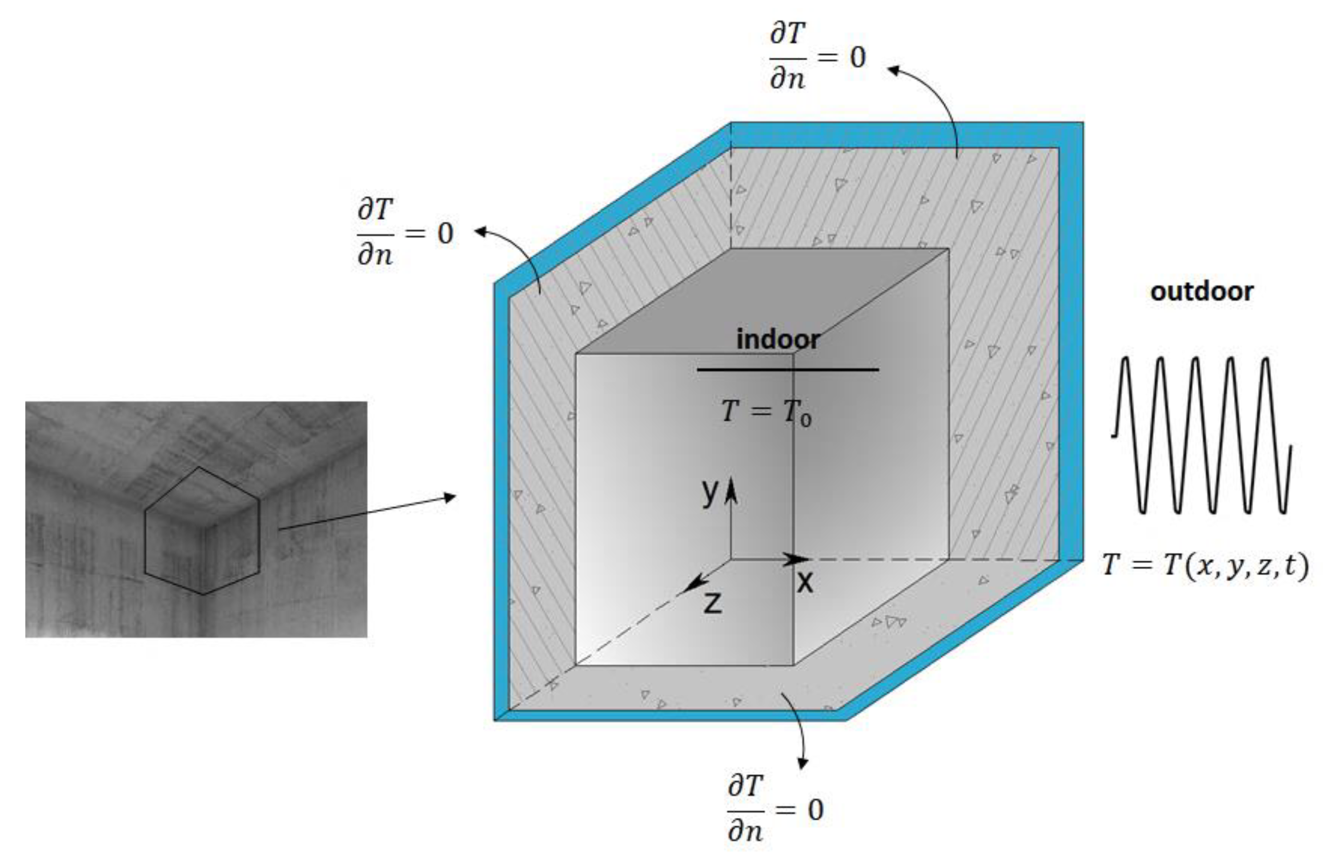
Three examples of a 3D concrete corner are simulated in terms of different scenarios for the thermal insulation layer (without thermal insulation, with an outer insulation layer, with an inner insulation layer) and the risk of moisture condensation is analyzed. The numerical simulations are performed considering that there is a sinusoidal variation of the external temperature over time (between −10 °C and 10 °C), while it is assumed that the internal temperature remains constant (20 °C). As the impact of the short-term environment moisture variation is limited to the outer surface layers of a wall, the indoor environment moisture conditions are kept constant (RH = 65%), and it is thus assumed that it does not influence the heat transfer across the wall [
43]. The dynamic heat flow rate through the PTB is compared with the dynamic heat flow rate through the LTBs and through the plane building elements (walls and roof). Furthermore, for each case study, the point thermal transmittance determined under steady state conditions is compared with the dynamic point thermal transmittance. The variation of the temperature distribution over time in different planes of the building corner domain is also analyzed. The internal surface temperature in the PTBs is compared with that in the wall and in the LTB junction to estimate the risk of condensation. The heat flux through the LTB is also compared with that through the PTB. By quantifying the surface temperature in the vicinity of PTBs, using the proposed 3D BEM dynamic models, this paper evaluates the risk of condensation by defining the temperature factor at the internal surface.
3. Validation of the Algorithm
The BEM formulation was validated experimentally. For that purpose, the dynamic heat transfer through a 3D wooden building corner, representing a PTB (3D junction between two walls and roof), was evaluated using a calibrated hot box. The experimental measurements and the numerical results are presented and compared in this section.
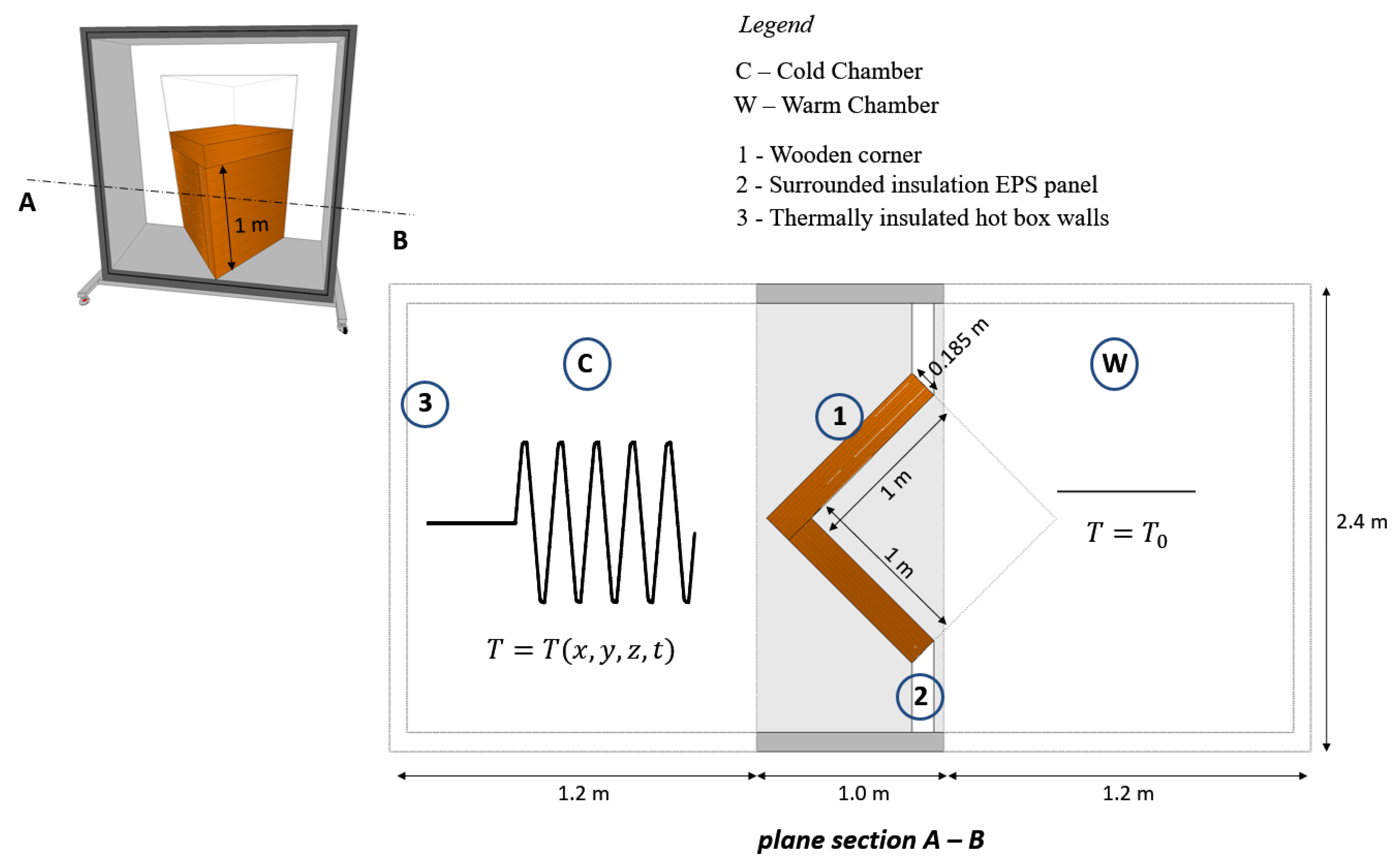
The wood solution was selected because it both represents a commonly used construction system, and it is light enough to be tested in a calibrated hot box. The specimen was placed inside a specially built large frame that was not designed to support heavy weights. This frame was then placed between the warm and cold chambers. The weight of the timber made it possible to build a corner composed of two walls 185 mm thick and 1.0 m long × 1.0 m high and a roof slab measuring 1.0 m × 1.0 m to inside the frame.
A 3D building corner was made from three dry CLT wood panels 0.18 m thick, 1 m wide and 1.5 m long.
Section 4 of
Table 1 lists the thermal properties of the CLT panels. It was assumed that the material’s properties were not dependent on the temperature and moisture content, given the small amplitude range of the temperatures.
The calibrated hot box apparatus was designed and built according to the specifications in ISO 8990:1994 [
33]. The 3D wooden corner was placed in an EPS surround panel between the two thermally insulated hot box chambers, one cold and the other hot, to allow heat to pass through the specimen (see
Figure 3). The hot and cold chambers each have an opening at the end to enable them to be connected, respectively, to a heating system and to a climatic chamber (Fitoclima 1000 from Aralab). The temperature required inside each one, for the test, is thus ensured. The cold chamber contains several fans to control the air flux velocity while the tests are in progress. The complete apparatus is set up in a laboratory environment under a controlled temperature (setpoint of 20 °C).
The experimental measurements required that the external surfaces of the wooden building corner undergo a variation of temperature, , but the setpoint temperature inside the warm chamber was kept constant .
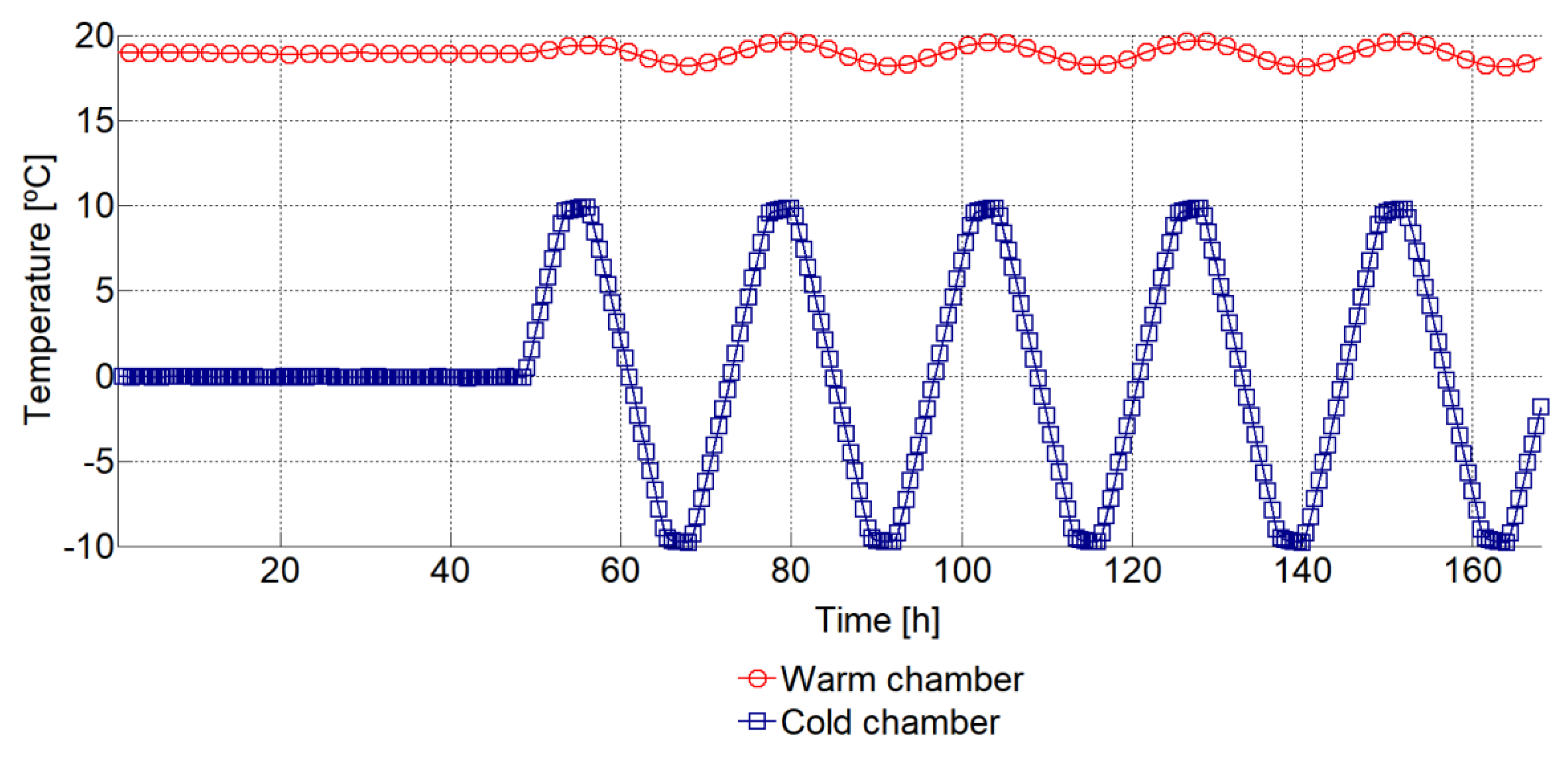
Figure 4 gives the variation of the imposed temperature over time, inside the two hot box chambers. The tests started with a period from
to
when the setpoint temperatures were kept constant inside the hot chamber (20 °C) and the cold chamber (0 ℃), so that steady state conditions were reached by the first time-step of the dynamic simulations. At the end of this period,
, the temperature variation started inside the cold chamber. For 24 h, the temperature–time dependence ranged between −10 °C and 10 °C, as shown in
Figure 4. In the warm chamber, the temperature setpoint was kept at 20 °C. The warm chamber could not be cooled, so the temperature inside it fluctuated between 18.2 °C and 19.7 °C. The real temperatures registered inside the warm and the cold chambers are given in
Figure 4. Five cycles were used for the experimental simulations.
The heat fluxes occurring though the internal surfaces of the wall (center of the vertical wood panel) were measured using an ultrathin flat plate heat flux sensor. This sensor consisted of thermoelectric laminated panels with a flexible heterogeneous plastic layer on either side.
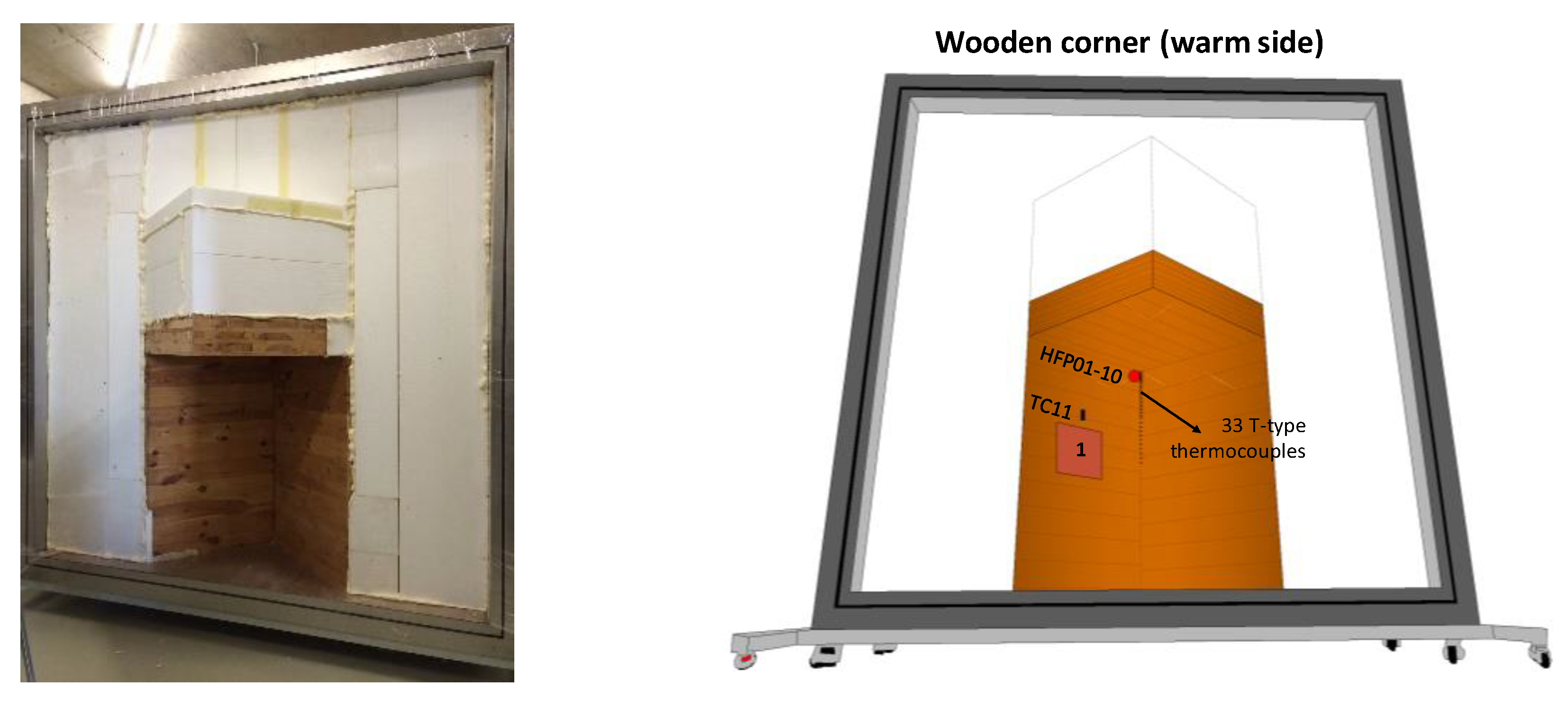
At the 3D corner, one HFP01 sensor [
47] from a Hukseflux TRSYS01 system [
48] measured the heat flux through the PTB, on the specimen’s warm side. The accuracy of HFP01 is ±5%. A GL820 Midi DataLogger recorded the data from the TRSYS01 system at 10-min intervals during the test. The internal surface temperatures in the center of the wood panels (roof and wall) were recorded on the warm side of the specimen by a pair of TRSYS01 thermocouples (TC12 and TC11, respectively).
At the PTB and the LTB, i.e., the junction between the two wood walls on the specimen’s warm side, the internal surface temperatures were recorded by 33 wire type T thermocouples, with a diameter less than 0.25 mm, in a vertical line at a distance of up to 0.32 m from the 3D corner. The uncertainty of each thermocouple was ±0.16 °C. Adhesive tape was used to fix them to the surface by an adhesive tape which had a high emissivity coating on its outer surface (>0.8), so that it would not affect the surface temperature measurements. A data logger system acquired the thermocouple temperature readings. Temperatures were recorded at 1 min intervals during the tests. All the components of the acquisition system were accurately calibrated prior to the tests.
Figure 5 shows the corner and the equipment layout.
The 3D BEM formulation (see
Section 2) was used for the numerical simulation of the heat transfer through the wooden corner, with the dynamic conditions being the same as those used in the experimental simulations (see
Figure 4).
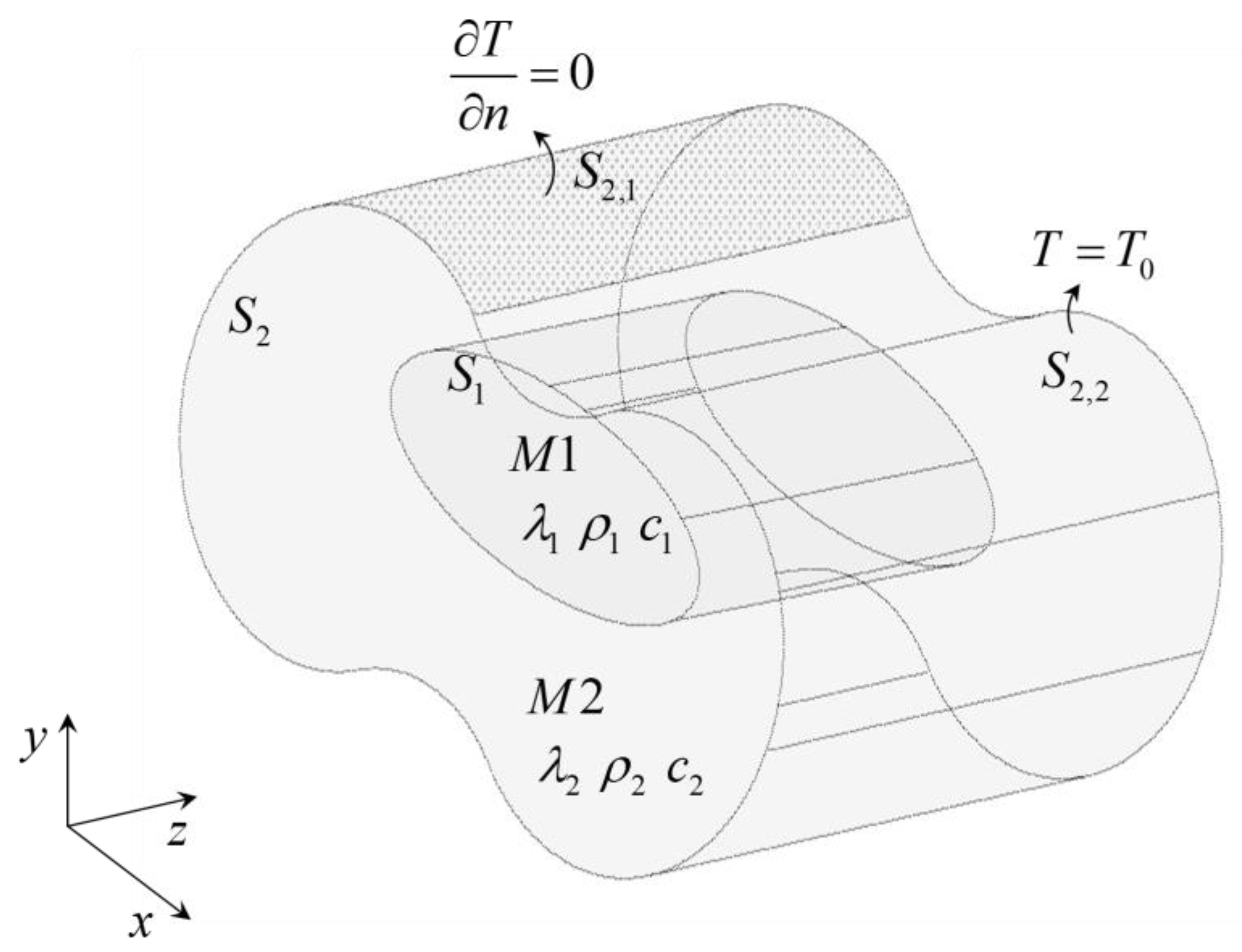
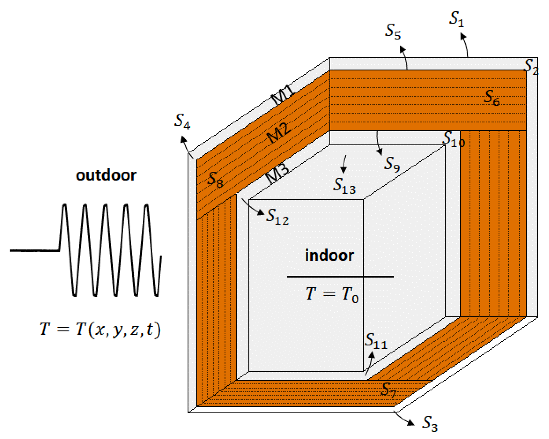
Figure 6 illustrates the 3D physical model of the problem. Medium M2 is the wood used for the corner, while medium M1 and medium M3 represent two thin air layers that account for the convection phenomenon on the outer surface and the radiation phenomenon on the inner surface of the corner.
Medium M1 is bounded by surfaces , , , and , medium M2 is bounded by surfaces , , , and , medium M3 is bounded by surfaces , , , and . Null heat fluxes are prescribed for the boundary cut-off surfaces , , , , , , , and and temperatures and are prescribed along the exterior boundary of the fictitious thin air layers (surfaces and ). The interfaces and are assumed to have continuity of heat fluxes and temperatures.
Different boundary meshes were used to ensure the convergence of the solution. These studies have not been included here for the sake of brevity, and only the final mesh configuration is presented. The interfaces between materials as well as the internal and the external boundary surfaces were discretized using 4563 constant boundary elements, and the modelling of the lateral surfaces at the cut-off planes of the building corner detail required 1872 constant boundary elements.
At it was assumed that the systems had a uniform temperature of °C throughout the entire domain. Note that non-uniform initial conditions could be imposed throughout the domain, but this would make the BEM model mathematically more elaborate. The range of frequencies used to compute the response was defined, so as to ensure that all significant contributions from all possible frequencies would be taken into account. The upper frequency of the analysis was set after it was confirmed that its contribution to the overall response would be negligible. The computation frequency domain ranged from Hz to Hz, and the frequency increment was Hz, and therefore the total time window for the analysis was 168.0 h.
The numerical simulations used 0.16 m2 °C/W and 0.14 m2 °C/W for the and values, at the wall surface. The experimental measurements were used to calculate these values. The convection/radiation effect is lower near the 2D and 3D corners, which led to higher thermal resistance at the surfaces. Near the PTB and LTB, the mean value estimated for the was 0.18 m2 °C/W.
The figures that follow give the heat fluxes and surface temperatures provided by the BEM under both steady state and dynamic conditions for a number of points on the internal and external surfaces of the wooden corner. The numerical results are compared with the experimental measurements.
Steady state conditions:
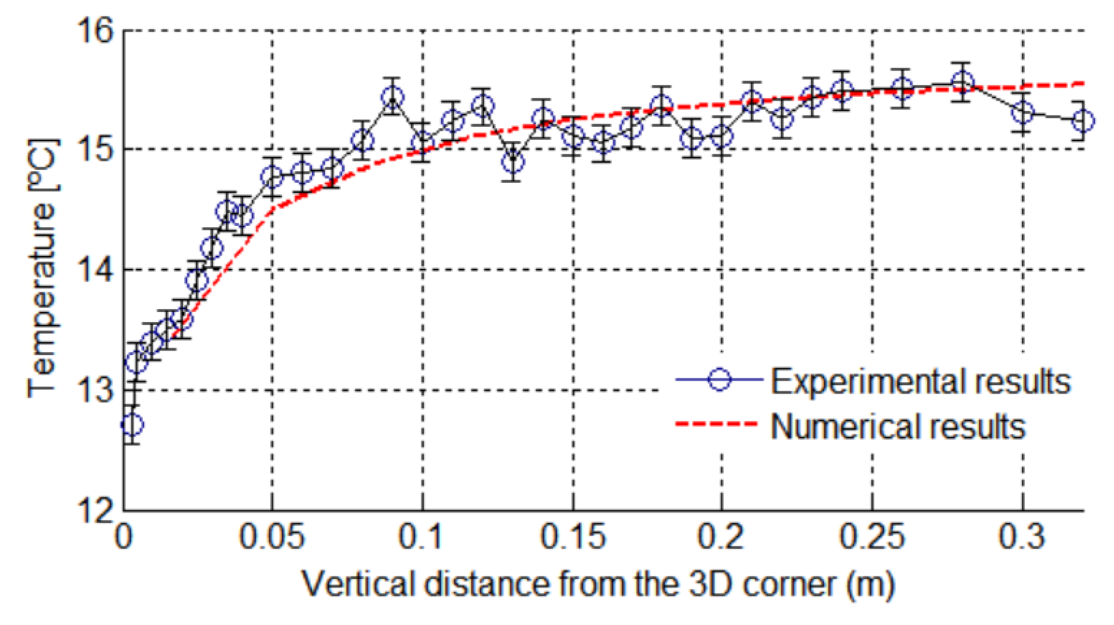
Figure 7 presents both the surface temperatures that the line of 33 type T thermocouples recorded and the surface temperatures obtained with BEM at the same points on the 3D corner and for the same constant conditions (19 °C in the hot chamber and 0 °C in the cold chamber). The error bar represents the uncertainty of each thermocouple (±0.16 °C). A good agreement can be seen between the measured values and numerical responses.
Steady state and unsteady state conditions:
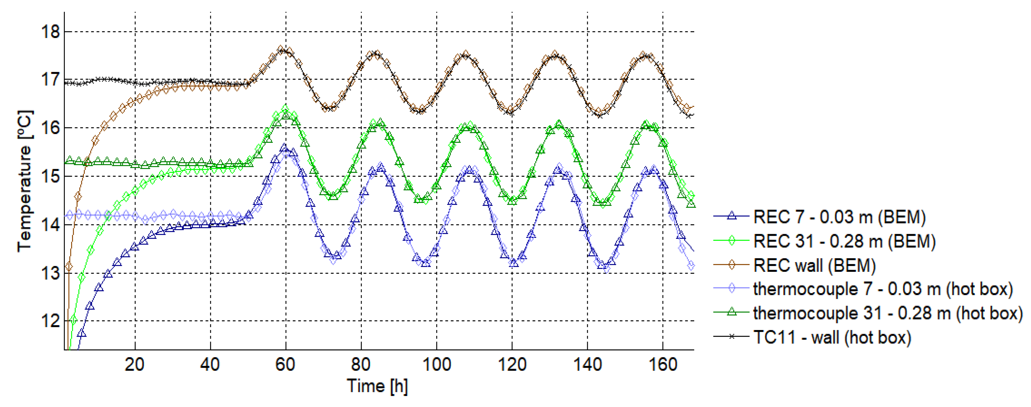
Figure 8 presents the internal surface temperature change over time. Two T-type thermocouples and the TC12 thermocouple from the TRSY01 system were selected to illustrate the results obtained. The thermocouple closest to the 3D corner is no. 7 (0.03 m), thermocouple 31 is in the 2D wall-to-wall junction, 0.28 m from the 3D corner and the TC12 thermocouple is in the center of the wall panel. The internal surface temperature given by the BEM for three receivers located in the same positions as the three thermocouples are also shown in
Figure 8. The experimental and numerical results were obtained under the dynamic conditions given in
Figure 4.
It takes a certain amount of time before the numerical responses achieved the steady state because the original conditions prescribed at were at a constant temperature of 0.0 °C throughout the physical domain. The two sets of values, experimental and numerical, subsequently show good agreement under the two sets of conditions.
The numerical responses obtained for the remaining points were also found to be in agreement with the experimental results.
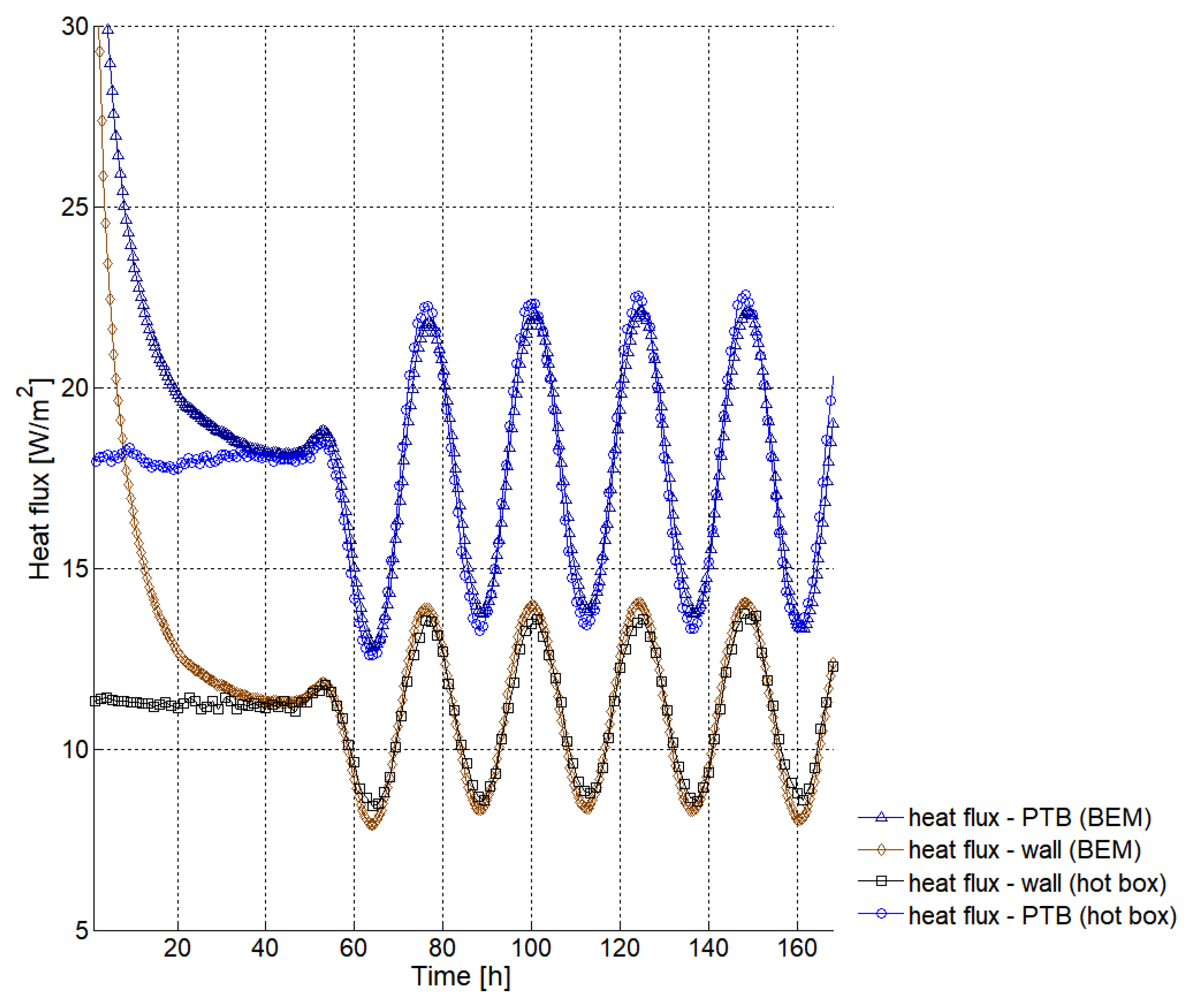
Figure 9 shows the heat flux changes on the warm surface of the wooden corner as time passes, values measured near the 3D corner (PTB) and in the center of the panel (wall). The numerical results and the experimental values are both given.
It can be seen that the heat flux curves obtained with the experimental measurements are in agreement with the heat flux curves obtained with the numerical simulation. The main differences between the BEM and the experimental results are observed in the local minimums and maximums of the heat flux curves, both in the PTB and in the center of the wall. These differences are, however, less than 0.5 W/m2, which is within the uncertainty range of the sensors (±5%).
Comparison of the experimental and numerical results confirms the reliability of the 3D BEM simulations and thus validates the proposed BEM model.
4. Numerical Application
After validation, we applied the 3D BEM formulation proposed in
Section 2 to simulate the heat transfer through a PTB formed at a 3D concrete building corner and evaluate the risk of condensation. First, the results for the steady state conditions are presented, followed by the results when the test specimen is subjected to unsteady state conditions.
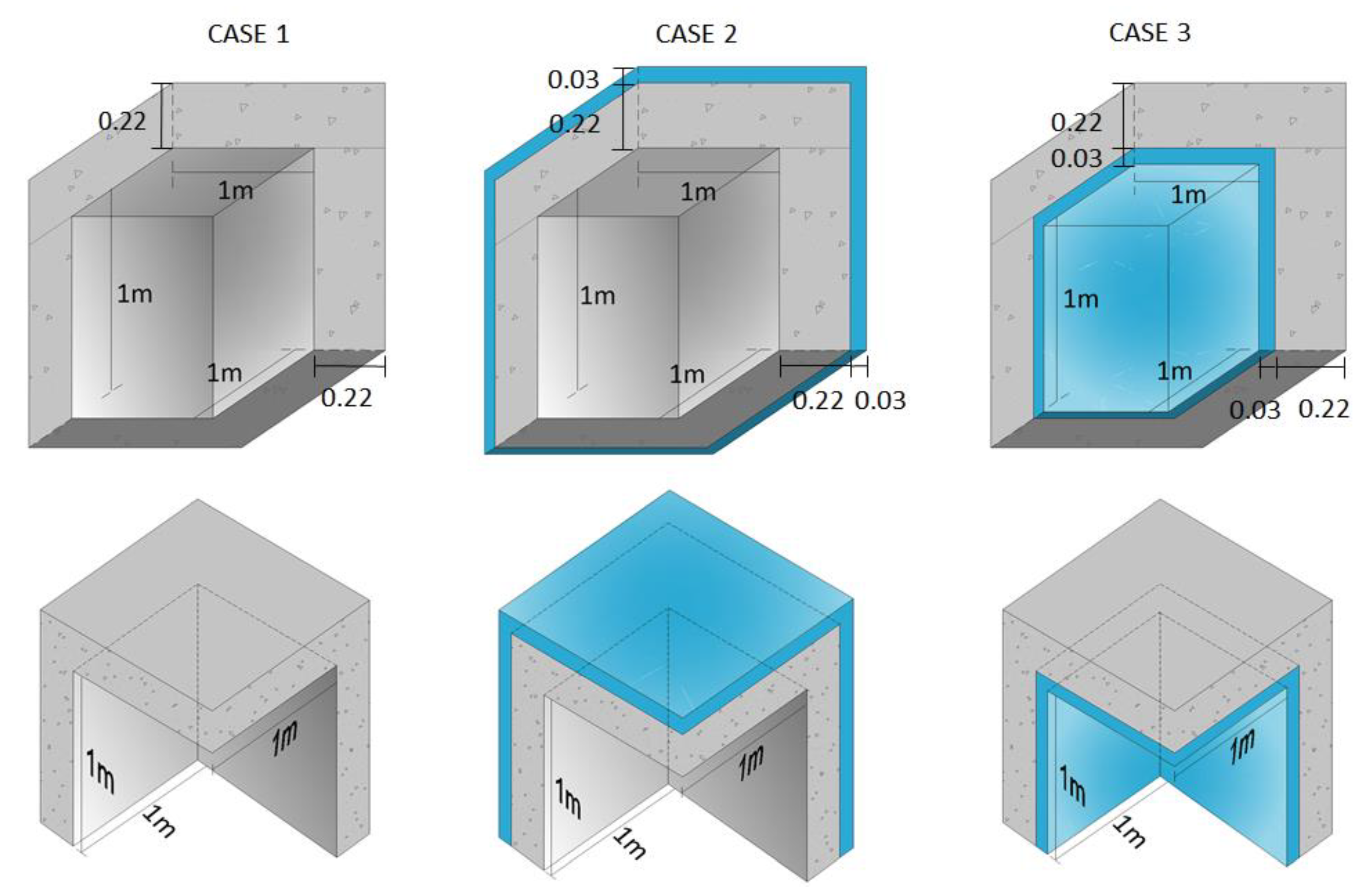
Figure 10 shows the three examples simulated: corner with no thermal insulation (Case 1); corner with outer layer of thermal insulation (Case 2); corner with layer of internal thermal insulation (Case 3).
The surface thermal resistance was modelled as a thin air layer on the inner and outer surfaces, thereby taking both the convection and radiation phenomena into account. The thermal resistance
on the inner surface depends on the direction of the heat flow [
49] which, under dynamic conditions, is liable to vary in time. However, in this study, the value
m
2 °C/W [
49] was used for all the internal surfaces, as indicated in ISO 10211:2007 [
1]. The external surface thermal resistance
was assumed to be 0.04 m
2 °C/W for the outer surfaces, according to ISO 6946:2007 [
49].
The 3D geometrical model of the building corner is delimited by cut-off planes. The cut-off planes are at a sufficient distance from the corner so that the point thermal bridge formed by the junction of the three building elements cannot affect the heat transfer. The length of the walls and roof in the three cases followed ISO 10211:2007, and a length of 1 m was therefore used.
The properties of each material, i.e., the thermal conductivity, mass density, and specific heat were characterized experimentally. The guarded hot-plate technique was used to evaluate thermal conductivity (ISO 8302:1991 [
50]). The apparatus used was a single-specimen Lambda-meter EP-500 from Lambda-Mebtechnik GmbH Dresden, and the test procedure set out in EN 12667:2001 [
51] was used. The procedure described in EN 1602:1996 [
52] was used to determine mass density, and the ratio method was used for specific heat, using an apparatus from Netzsch, model DSC200F3. Five tests specimens were used for each test procedure. The average values of and standard deviations found for the thermal properties of the materials are given in
Table 1. All tests were performed at ITeCons - Institute for Research and Technological Development in Construction, Energy, Environment and Sustainability, an accredited laboratory for a wide range of tests.
4.1. Steady State Conditions
The importance of dynamically computing the PTB was confirmed by first solving the problem assuming that a steady state condition prevailed. This corresponded to the static response. The computation of the quantity describing the influence of the PTB on the total heat flow, in W/°C, i.e., point thermal transmittance
, required setting specific outdoor and indoor temperatures,
and
, respectively, which were held to be time independent. The following equation was used, in accordance with ISO 10211:2007 [
1]:
in which
is the number of plane building elements,
is the number of 2D junctions between plane elements,
is the thermal coupling coefficient yielded by the three-dimension calculation, in W/°C, computed for the total system (see
Figure 11a),
is the total heat flow rate in W, computed with the proposed BEM model,
is the thermal transmittance (in W/(m
2 °C) of the plane building element
separating the internal and the external environment,
is the rate of heat flow, in W/m
2, for the 1D plane element
, and
is the area (in m
2) for which the
is applicable,
is the linear thermal transmittance (in W/(m °C)) of the junction
between two building components, representing an LTB, and
is the length to which
applies.
The linear thermal transmittance
of each LTB was computed as
where
is the coefficient of thermal coupling given by a 2D calculation of the LTB detailed
, in W/(m°C) and
is the rate of heat flow per meter length, occurring through the LTB detail
, computed with the proposed BEM model.
Figure 11b–d gives the different details of LTB considered in the application of Equations (9) and (10).
The thermal coupling coefficients and were determined by integrating the heat fluxes along the inner surfaces of the components. However, the same result could be achieved if any other integration line were used, because the simulation of the systems assumed steady state conditions.
In the three case studies and , since the constructive details and the surface thermal resistances were assumed to be the same for the three 1D components of the building corner.
The computations in steady state were performed with the proposed BEM formulation, and null frequency was imposed with a small imaginary part, , where is almost zero, .
Each interface between materials was discretized by 4563 constant boundary elements, while the lateral interfaces at the cut off planes were modelled by 1872 constant boundary elements.
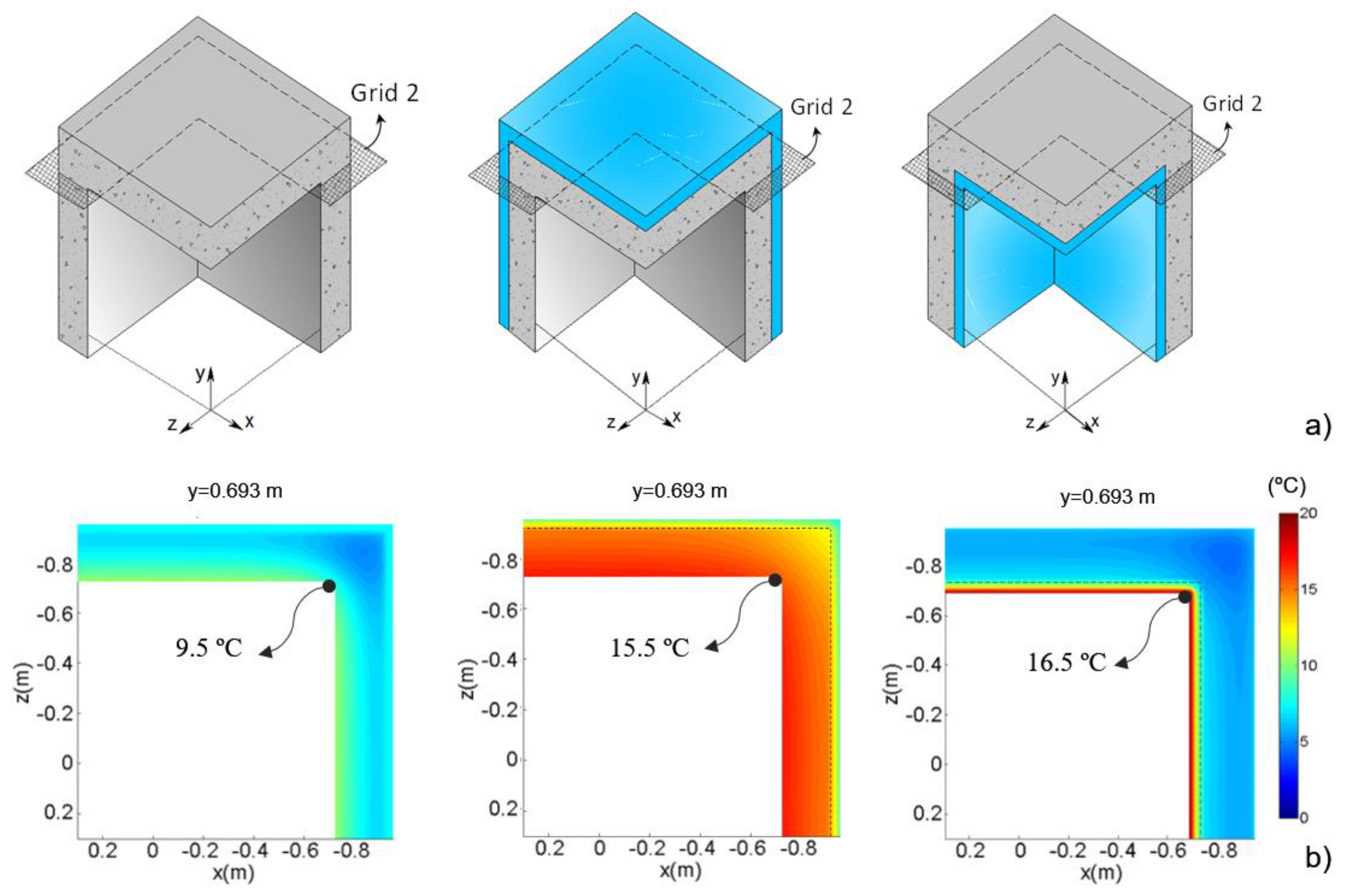
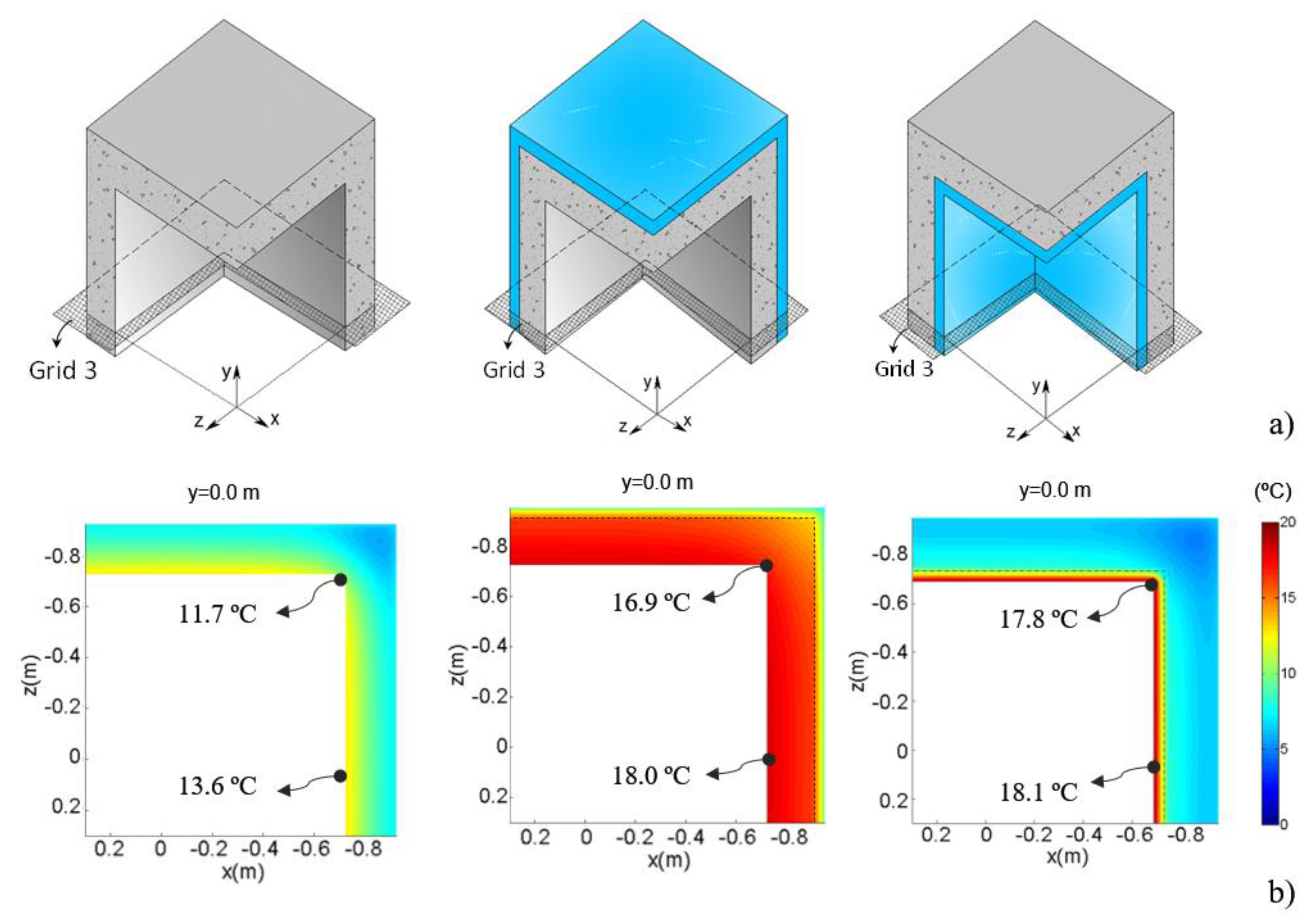
Six very fine grids of receivers were used to measure the temperature distribution. They were placed as shown in
Figure 12.
Grid 1 is a longitudinal square grid along the internal surface of the concrete roof and the plane sections between roof and walls. Grid 2 is a longitudinal grid crossing the 2D corner corresponding to the wall-to-wall junction, 0.01 m from the 3D corner. Grid 3 is similar to the grid 2 but placed 0.7 m from the 3D corner. Grid 4 contains three different planes of grid receivers lying in the planes of the two walls and roof internal surfaces of the 3D building corner detail. Grids 5 and 6 are similar to Grid 4 but placed in different locations depending on the case study. In Case 1, Grid 5 and Grid 6 are placed inside the concrete, 0.06 m and 0.17 m from the internal surface, respectively; in Case 2, Grid 5 is placed in the middle of the insulation layer and Grid 6 in the middle of the concrete layer; in Case 3, Grid 5 is placed in the middle of the concrete layer and Grid 6 in the middle of the insulation layer.
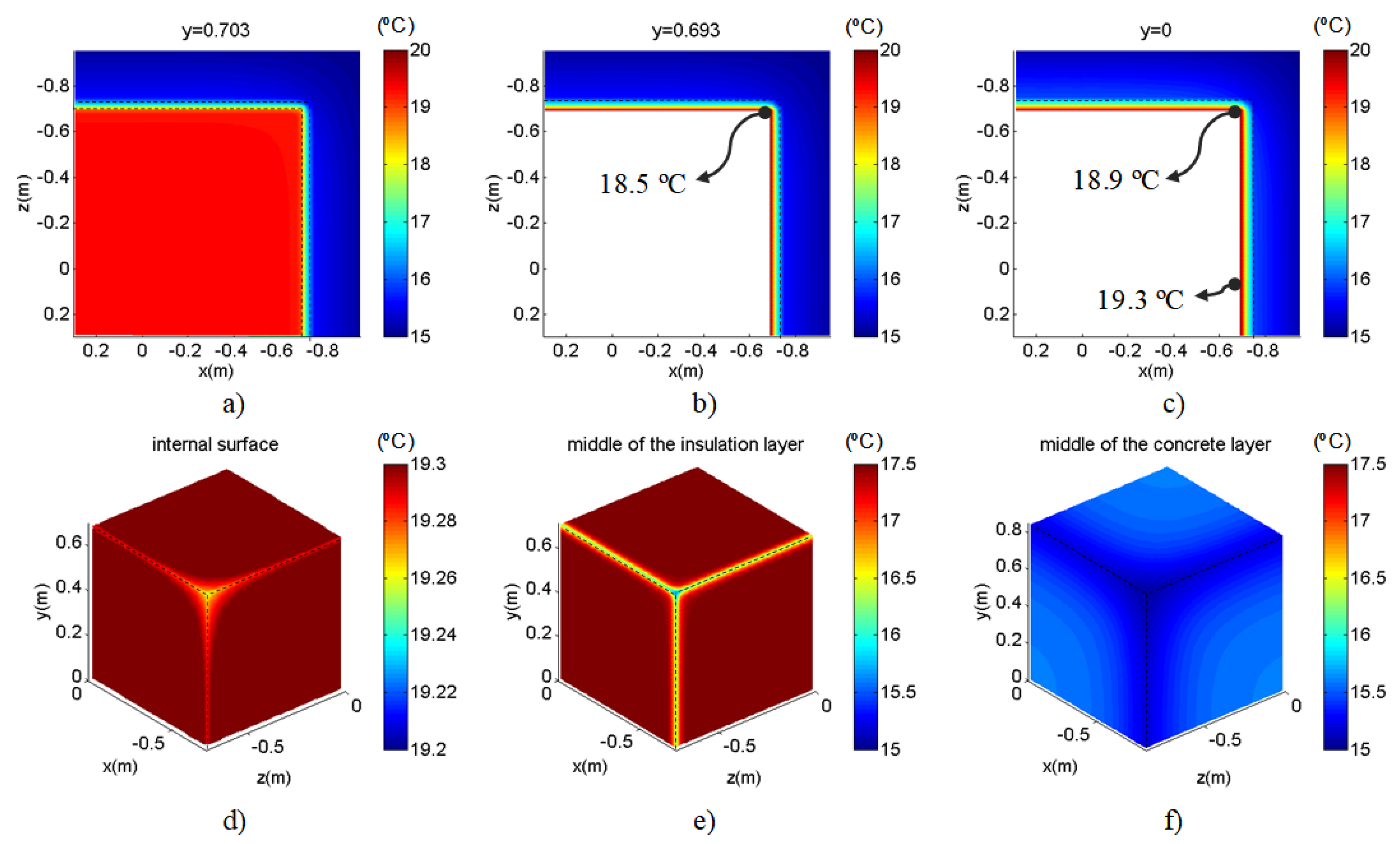
Figure 13,
Figure 14 and
Figure 15 show the temperature distribution recorded at each grid of receivers in case studies 1, 2, and 3, respectively, under steady state conditions in which the interior temperature was 20 °C and the exterior temperature was 15 °C. In the color scale used in the plots, the red shades signify higher temperatures and blue shades indicate lower temperatures. As expected, analysis of the results showed that the surface temperatures in Case 1 were lower surface temperatures. The lowest temperatures within the wall were recorded for Case 3, in the middle of the concrete layer. The PTB effect on the temperature distribution is clearly visible in the three cases.
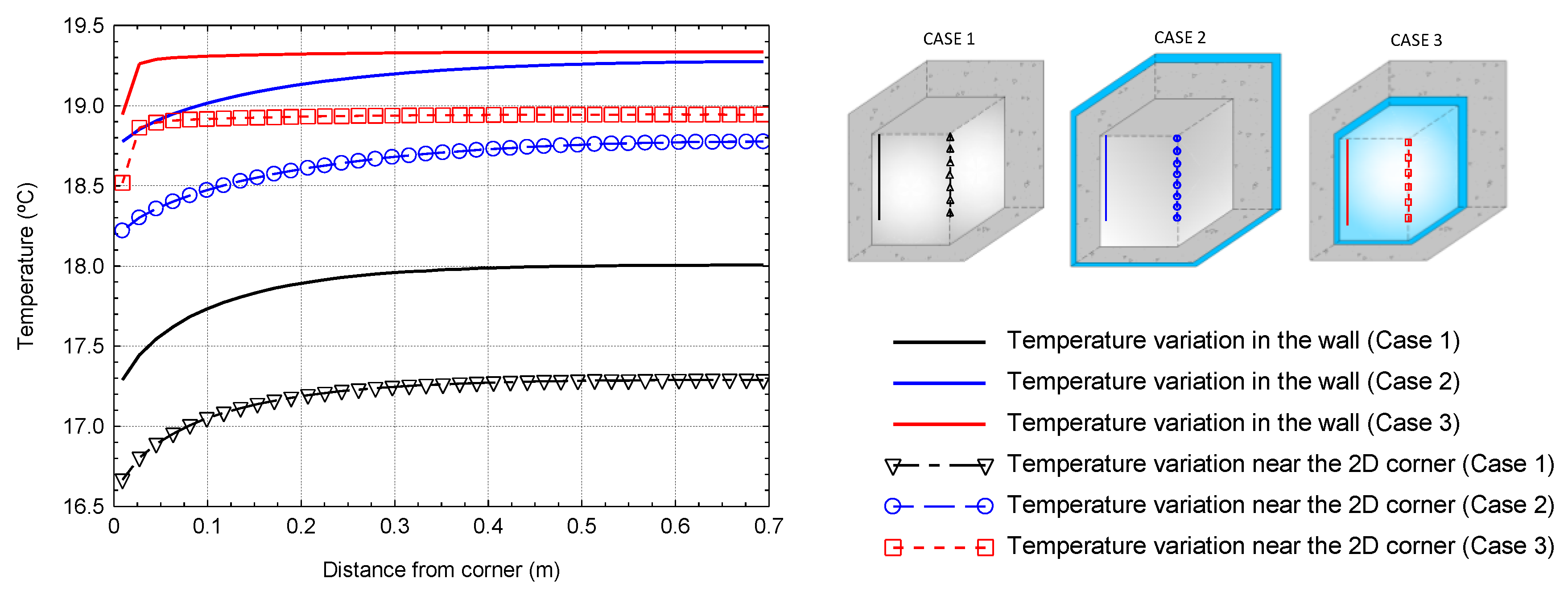
Figure 16 gives the variation of the internal surface temperature along two different sections of the building corner, when steady state conditions are assumed. The dashed lines with marks illustrate the internal surface temperature along the LTB junction, starting in the 3D corner. The straight lines present the internal surface temperature along the wall, starting in the 2D corner. Different colors identify each case study results (Case 1—black lines; Case 2—blue lines; Case 3—red lines).
It can be seen that in the three case studies, the lowest surface temperatures are registered where there is a more marked thermal bridging effect, i.e., near the 3D corner. The difference between the surface temperatures in the 3D corner and in the middle of the wall is greater in Case 1 (0.7 °C) and lower in Case 2 (0.4 °C). Note that these results were obtained for a temperature gradient of 5 °C between the internal and the external environment, and therefore these values will tend to increase for the highest temperature gradients that typically occur in the winter.
The condensation risk can be evaluated by comparing the temperature factor at the internal surface with the limit, which needs to be defined for each climate. The calculation of the limit is based on the temperature and relative humidity data and on the required interior environment conditions. The occupancy level and activity should also be taken into account.
The factor is given by the following equation
This factor is very useful to characterize the thermal quality of building details. Lower
values are associated with lower surface temperatures and the consequently higher risk of surface condensation [
53]. If it occurs it can cause mold growth and damage coatings. For example, to prevent mold growth in the United Kingdom
should be greater than 0.75 [
54] and for some climate zones in Switzerland
should be greater than 0.78 [
55].
Moreover,
is used to determine the temperature on the inner surface
for any temperature gradient from the indoor to the outdoor environment
[
1].
Table 2 gives the temperature factors at the internal surfaces
of the wall, LTB and PTB of the 3D building corner being studied, obtained by the following equation:
Table 2 shows that the
values are significantly lower near the 3D corner (in the PTB) than at the wall surface, even when thermal insulation is applied. Indeed, these values are lower than 0.75, the minimum acceptable according to [
54].
Table 3 gives the results of computing the point thermal transmittance of the three case studies. Case 2 shows the greatest point thermal bridge contribution with
W/°C. The static point thermal transmittance is lower in Case 3 (
W/°C).
As expected, it can be concluded that, for all the case studies, when the conditions are steady state, the point thermal bridge is negligible in terms of heat losses. However, this calculation is useful to assess the risk of moisture condensation. Particularly since, as we can see in
Figure 16, the surface temperature near the 3D corner is clearly lower than the surface temperature at the center of the 1D building element and in the LTB junctions.
4.2. Unsteady State Conditions
The new 3D BEM model was then run to simulate the dynamic conduction heat transfer through the three building corner details presented in
Figure 10. For this, at
, a uniform temperature of 20 °C was assumed for the three physical models, throughout the entire domain. At
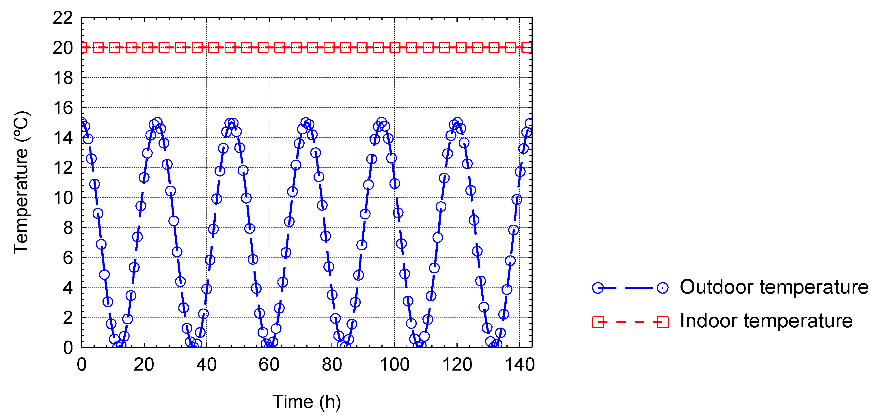
all the models underwent an exterior temperature change. A sinusoidal temperature time dependence was assumed; the cycle lasted 24 h and had temperature amplitude oscillations of 15 °C, as shown in
Figure 17. Six cycles were simulated, so that the system response would achieve a cyclic behavior over time.
The frequency domain of computation ranged from 0.0 Hz to Hz, with a frequency increment of Hz. The total time window for the analysis was therefore 144 h. This test used the same boundary discretization for the BEM model as described above. The same receiver grids used for the steady state response were used to compute the temperature distribution. The resulting heat diffusion across the point thermal bridge is illustrated by a series of snapshots of the simulations of the time domain.
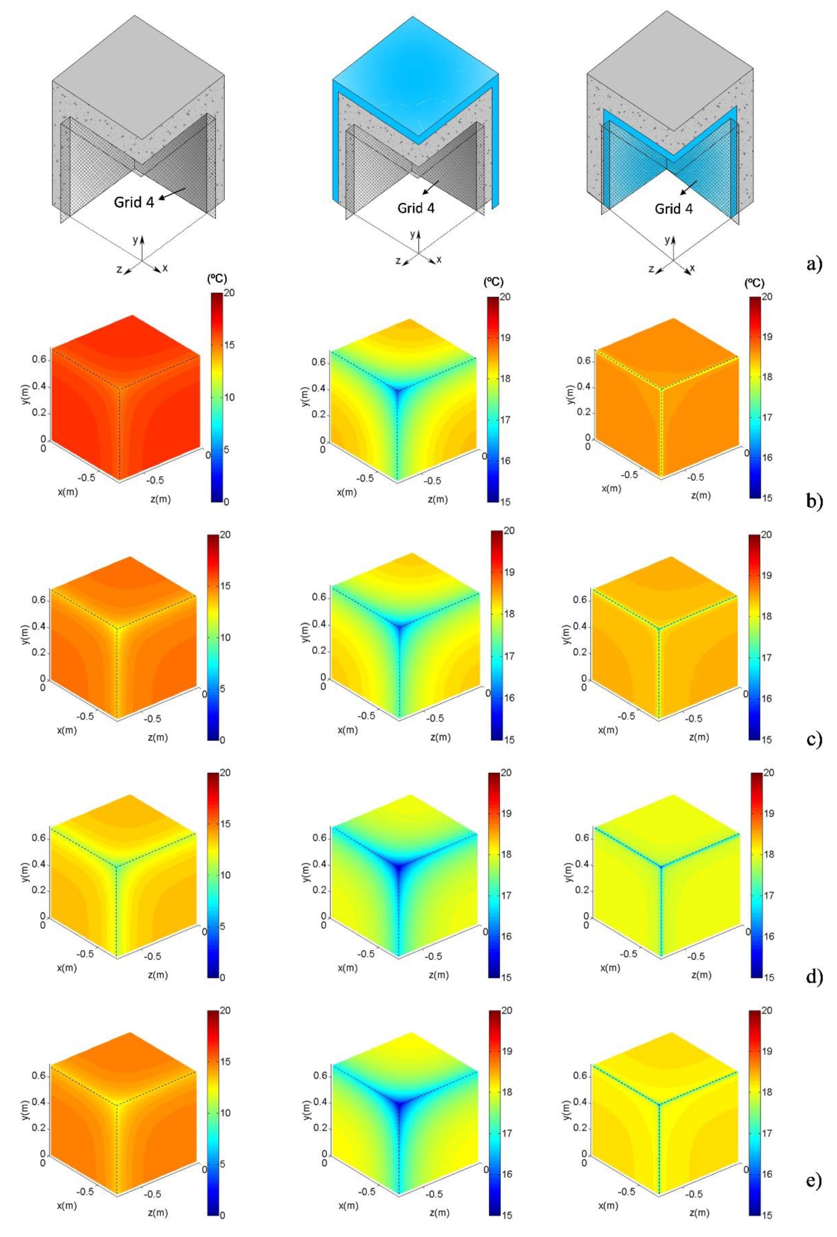
The temperature field distribution at Grid 4 is shown in
Figure 18, for the three cases at four time instants: (b)
t ≈ 102 h; (c)
t ≈ 108 h; (d)
t≈ 114 h and (e)
t ≈ 120 h).
Figure 19 and
Figure 20 give the temperature field distribution at Grid 2 and Grid 3, respectively, for the three cases at time instant
t ≈ 114 h. The color scale used in the plots is the same as before, with the red shades being the higher and the blue shades the lower temperatures.
At
t ≈ 102 h (
Figure 18b), the penultimate 24 h cycle of the exterior temperature had already started, and the temperature had dropped from 15 °C to 7.5 °C. At this instant, the point thermal bridging effect is barely perceptible in the plots of Cases 1 and 3. As expected, the surface temperature near the PTB is lower in Case 1 (14.7 °C) than in Case 2 (16.1 °C) and Case 3 (17.9 °C). The thermal gradient between the internal surface near the 3D corner and the internal surface in the wall is about 1.8 °C in Case 1, 2.3 °C in Case 2, and 0.9 °C in Case 3.
At
t ≈ 108 h (
Figure 18c), the exterior temperature stood at 0 °C and the surface temperatures were falling throughout the Case 1 domain (no thermal insulation). The point thermal bridging effect in the temperature distribution was now clearly visible near the 3D corner in Cases 1 and 2. The surface temperature in Case 1 decreased almost 3 °C in the PTB, 2 °C in the LTB and 1.4 °C in the wall, when compared with the first plot. In Cases 2 and 3, the decrease was less marked because of the effect of the thermal insulation.
At
t ≈ 114 h (
Figure 18d and
Figure 19d to
Figure 20d) the exterior temperature stood at 7.5 °C. However, it was still falling at the grid of receivers and reached the lowest values at the internal surfaces in the three cases. The point thermal bridging effect is now very pronounced, thus leading to significantly lower temperatures in the vicinity of the 3D corner. In Case 2, the internal insulation acts as a barrier to the heat transfer and the temperatures in the concrete layer practically did not vary. In Cases 1 and 2 these plots also showed the thermal inertia effect of the material in the interior domain of the PTB. In Case 1, the lack of thermal insulation lead to significantly lower surface temperatures than in the other two cases. This difference is 7 °C near the PTB and 6 °C in the vicinity of the LTB.
At
t ≈ 120 h (
Figure 18e) the exterior temperature had reached again 15 °C, completing the penultimate cycle of 24 h. The temperature is now increasing through the full domain of the three case studies. However, this is still barely perceptible at the internal surface of Case 2.
The figure also shows that, in the four instants analyzed, the PTB and LTB surface temperatures are higher in Case 3 (which has an internal layer of thermal insulation).
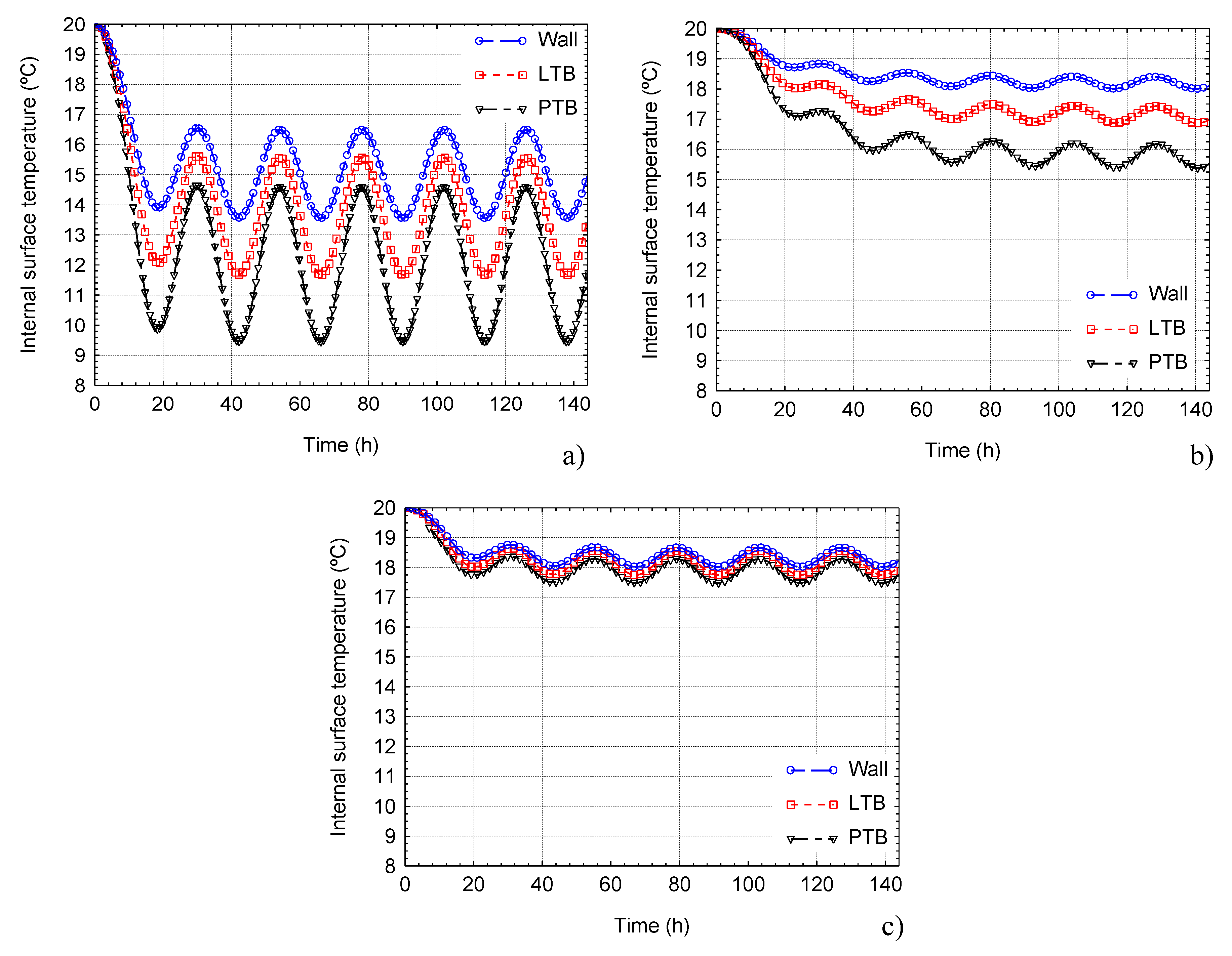
Figure 21 presents the internal surface temperature variation over time in the PTB (black curve), the LTB (red curve) and in the plane wall (blue curve), obtained for each case study (Case 1—a); Case 2—b); Case 3—c)). We can see that the surface temperatures are significantly lower near the 3D corner (in the PTB) and highest at the plane wall, in all three studies. The thermal amplitude of the surface temperature over time is higher in the PTB, especially in Case 1, without thermal insulation (
Figure 21a).
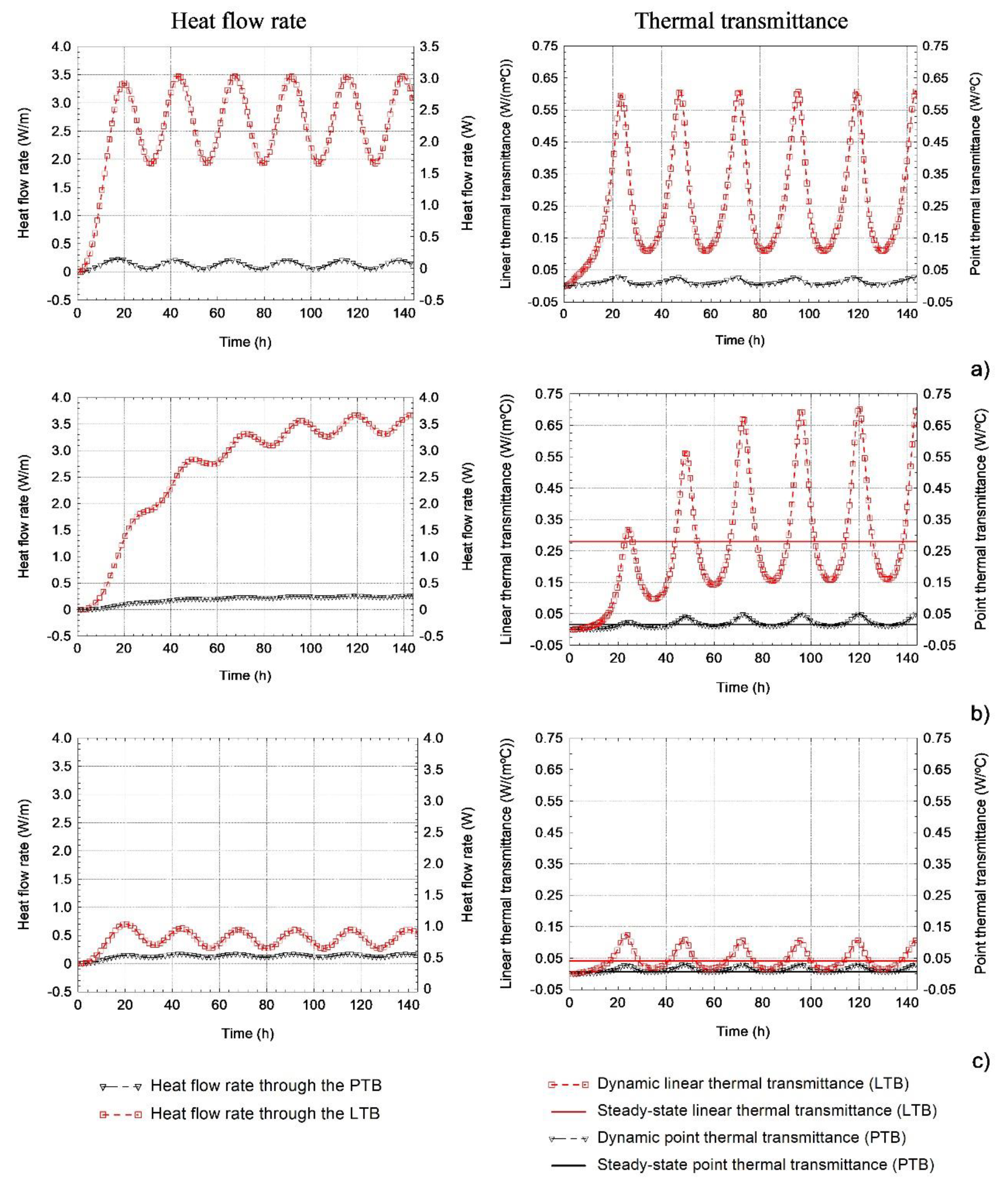
The plots in
Figure 22 present the change in heat flow rate per meter length through the LTB
and the heat flow rate through the PTB
, as well as the variation of the dynamic linear and point thermal transmittances (
and
, respectively), over time, obtained for the three case studies.
The method adopted for computing and differed slightly from the one used for steady state conditions. This is because the problem is dynamic and, so, care is needed with respect to the position of the planes over which the global heat flux is computed, since the dynamic effects lead to individual values. The inner surfaces were selected because moisture condensation and pathologies are often on these surfaces, and they are important in the evaluation of the dynamic heat flow.
As expected, for the three case studies, the heat flow rates through the PTB are significantly lower than those through the LTB. It can also be seen that the difference between the point thermal transmittances obtained under dynamic and steady state conditions is not very significant, since both steady state and dynamic heat fluxes are very low. Furthermore, the heat loss through the PTB occurs only at a point, whereas the linear heat loss occurs throughout the whole length of the LTBs. Therefore, it can be concluded that, for the three cases analyzed in this study, the PTB can be neglected in terms of heat loss. However, the evaluation of the dynamic behavior of PTB details is important to prevent moisture condensation problems, since it enables the evaluation of minimum surface temperatures over time, and therefore higher performance solutions can be studied and proposed.


