Novel Proposal for Prediction of CO₂ Course and Occupancy Recognition in Intelligent Buildings within IoT

Abstract

Many direct and indirect methods, processes, and sensors available on the market today are used to monitor the occupancy of selected Intelligent Building (IB) premises and the living activities of IB residents. By recognizing the occupancy of individual spaces in IB, IB can be optimally automated in conjunction with energy savings. This article proposes a novel method of indirect occupancy monitoring using CO₂, temperature, and relative humidity measured by means of standard operating measurements using the KNX (Konnex (standard EN 50090, ISO/IEC 14543)) technology to monitor laboratory room occupancy in an intelligent building within the Internet of Things (IoT). The article further describes the design and creation of a Software (SW) tool for ensuring connectivity of the KNX technology and the IoT IBM Watson platform in real-time for storing and visualization of the values measured using a Message Queuing Telemetry Transport (MQTT) protocol and data storage into a CouchDB type database. As part of the proposed occupancy determination method, the prediction of the course of CO₂ concentration from the measured temperature and relative humidity values were performed using mathematical methods of Linear Regression, Neural Networks, and Random Tree (using IBM SPSS Modeler) with an accuracy higher than 90%. To increase the accuracy of the prediction, the application of suppression of additive noise from the CO₂ signal predicted by CO₂ using the Least mean squares (LMS) algorithm in adaptive filtering (AF) method was used within the newly designed method. In selected experiments, the prediction accuracy with LMS adaptive filtration was better than 95%.

1. Introduction

Until recently, automated smart wiring was the privilege of commercial buildings. However, more and more people want to take advantage of the smart installation options in their homes. There are already many companies on the market involved in smart installations. The prices of such systems with high level of reliability are becoming more affordable in relation to what the customer gains. One of the customer’s motivations for monitoring and controlling the operational and technical conditions of the building can be tracking the events in the building. By measuring various physical quantities, for example, a window left open, unauthorized entry or the presence of people in a building can be inferred. Another motivation for space monitoring can be care for disabled people or seniors. The IoT is increasingly being used to monitor and control the operational status of a building today, which greatly facilitates remote communication with the building from anywhere in the world. This is an area that is relatively new and constantly developing. However, multinational companies such as Google, IBM, Amazon, etc. are becoming increasingly important players in the IoT world. They come with their services, which they run on their servers and offer to customers. These services are generally referred to as Cloud Computing (CC). IB and IoT are two distinct concepts that are closely related, as IB requires real-time interaction with different technological processes. The interactions take place within the system on the basis of a programmed model or directly with the users, and IoT inherently helps. This research is focused on current trends in building automation and monitoring of operational and technical conditions in IB within IoT. The authors of [1,2,3,4,5,6,7,8,9,10,11,12,13,14,15,16,17,18,19,20,21,22,23] focused on new approaches for home automation solutions within IoT. The authors investigated the new possibilities and trends of IB and smart home (SH) automation solutions with appropriate use of IBM IoT tools [2,3,4,5,6], with ensuring appropriate security in IB and SH automatization [7,8,9], and with the possible overlap of applications within the Smart Cities (SC) [10,11] and Smart Home Care (SHC) [12] platforms.

The above-stated articles contain technical terms such as SH, IB, IoT, communication technology, data transfer in connection with communication protocols, CC, “Cloud of Things”. etc. SH is an automated or intelligent home. This is an expression for a modern living space in contrast to existing conventional buildings. SH is characterized by a high degree of automation of operational and technical processes, which are operated by people in standard households. These include lighting control, air temperature and air-conditioning control, kitchen equipment, security technology, door and window control, energy management, multimedia, and consumer electronics control, among many others. SH connects a number of automated systems and appliances with interoperability among the decentralized or centralized management technologies used. One of the main objectives is to increase the required level of user comfort while saving energy costs [24]. SH should, of course, also offer the possibility of an additional configuration of functionality.

IoT is a network of interconnected devices that can exchange information with each other and be mutually interactive. Each of these devices must be clearly identifiable and addressable. Standardized communication protocols are used for communication. The aim is to create autonomous systems that are able to perform the expected activities completely independently on the basis of data obtained from the equipment. In practice, this means that the more data are collected, the better they can be analyzed, which may be useful in IoT implementation in specific fields [25]. In his article on the introduction to the IoT, Vojacek described IoT architecture as a model consisting of three basic elements [26]. The first block includes the “things” themselves, which are all devices connected to the network, whether cable or wireless, providing completely independent data. The second block represents the network, which serves as a means of communication between the things themselves and the control system. The third block includes data processing, which can be on the cloud, i.e. a remote server on which the data are further processed. The development of the Internet of Things is now mainly driven by the rapid development of new IoT-enabled devices and their ever-decreasing price. By 2020, it is estimated that the number of connected IoT devices may exceed 30 billion [27]. However, this figure varies for different sources, but it is certain that the numbers go to tens of billions. This brings about the issue of Internet addressing, because addresses from the IPv4 address space were depleted in 2011, but, with the advent of IPv6, address depletion should not occur as there are $2^{128}$ addresses in this address space, which is a huge number; for your information, it is about 66 trillion IP addresses per square centimeter of the Earth’s surface, including the oceans [28,29]. The Internet of Things may be used in many sectors of human activities. Smart Cities (SC) and Smart Grids (SG) can also be included in the current IoT application areas.

Obviously, it is necessary to transfer the data collected effectively. When it comes to wireless data transmissions, the most important parameters include especially range, energy intensity, the security of transmission, format, intensity of data processing, and transmission speed. Competition in this segment is relatively high [30,31,32,33]. Several communication protocols, such as MQTT, Constrained Application Protocol (CoAP), and Extensible Messaging and Presence Protocol (XMPP), are available for IoT data transmission [34]. In this work, the MQTT protocol is used. Aazam et al. described the topic of CC in the work “Cloud of Things: Integrating the Internet of Things and CC and the issues involved” [35]. This is a growing trend in IT technologies, which is also used in IoT. The characteristic feature of CC is the provision of services, software, and hardware of servers that are accessible to the users via the Internet from anywhere in the world. The cloud technology provider will enable the user to use their computing power, data storage, and the software offered. For the users, these services are appealing because they may not have the knowledge of the intrinsic functionality of the hardware and software leased. It also offers high-level data security or a high-quality, user-friendly web interface. Depending on the use of services, CC can be divided into groups [36]: IaaS (Infrastructure as a Service), SaaS (Software as a Service), PaaS (Platform as a Service), and NaaS (Network as a Service). The basic idea behind CC is to move application logic to remote servers. The individual devices in SH with an Internet connection can be connected directly to the cloud. The data received are collected and processed here. Based on the data evaluated, there is a feedback interaction with the devices in SH. It is often necessary to connect a device that does not have an Internet connection to the system. This can be performed using a gateway that is connected to the Internet. This gateway does not have to mediate communication to only one device. Often, cloud services also offer their own applications for visualization of the data processed and their storage in the database. There is a huge amount of data that can be used for other complex calculations, such as machine learning. Leading providers of these cloud technologies include IBM, which, inter alia, offers IBM Watson IoT, and Amazon with its Amazon Web Services.

Similar to this study, the obtained results in [12,18,37,38] showed that the accuracy of CO₂ prediction can possibly exceed 90%. Khazaei [39] employed a multilayer perceptron neural network for the purpose of indoor CO₂ concentration levels, where relative humidity and temperature were used as inputs. The most accurate model (based on the calculated mean-square-error (MSE)) was five steps ahead of the reference signal. On average, the difference between reference and prediction signals was less than 17 ppm. Wang [40] used a recurrent neural network (RNN) based dynamic backpropagation (BP) algorithm model with historical internal inputs. The models were developed to predict the temperature and humidity of a solar greenhouse. The obtained results demonstrate that the RNN-BP model provides reasonably good predictions. One of the benefits of the prediction of CO₂ concentration levels is low-cost indirect occupancy monitoring. Szczurek et al. proposed a method to provide occupancy determination in intermittently occupied space in real-time and with predefined temporal resolution [41]. Galda et al. 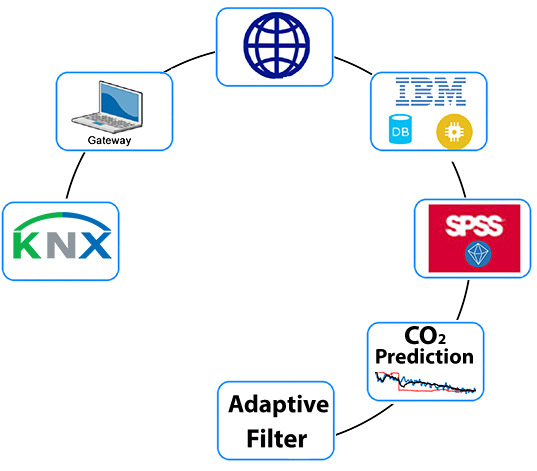discovered insignificant difference between a room with and without plants, while measuring values of CO₂ concentration, inner temperature, and relative humidity [42]. In our article, we used KNX technology for IB–IoT connectivity by means of the MQTT protocol within the IBM Watson IoT platform. The target of this article is to propose and verify a novel method for predicting CO₂ concentration (ppm) course from the temperature (T_indoor (°C)) and relative humidity (rH_indoor (%)) courses measured with operational accuracy to monitor occupancy in SH using conventional KNX operating sensors with the least investment cost. To achieve the goal, it is necessary to program the required KNX modules in the ETS 5 SW tool. Next, a software application is created to ensure connectivity between the KNX technology and the IoT IBM platform for real-time storage and visualization of the data measured. To predict the course of CO₂ concentration, it is necessary to verify and compare mathematical methods (linear regression (LR), random trees (RT), and multilayer perceptron’s (MLP)), and to select the method with the best results achieved. To increase the accuracy of CO₂ prediction, it is necessary to implement the LMS AF in an application for suppressing the additive noise from the CO₂ signal predicted and to assess the advantages and disadvantages of using AF in the newly proposed method. The proposed method was verified using the measured data in springtime with day-long and week-long intervals (2–10 May 2019). The proposed method can save investment costs in the design of large office buildings. Recognition of occupancy of monitored premises in the building leads to the optimization of IB automation in connection with the reduction of operating costs of IB.

2. Materials and Methods

2.1. Building Automation—KNX Technology

KNX technology is a worldwide standard in the field of wiring of intelligent buildings and their automation. It is a decentralized solution. KNX technology provides the interconnection of KNX modules using the Twisted pair (TP) communication medium. The devices used in this work are an MTN6005-0001 sensor of CO₂, temperature, and air humidity (technical parameters: current consumption from the bus, max. 10 mA; ambient temperature, −5 to 45 °C; measuring range for CO₂, 300–9999 ppm; measuring range for temperature: 0–40 °C; and measuring range for humidity, linear 20–$100\%$). A laboratory (EB312) on the premises of the building of the new FEI at VSB Technical University of Ostrava was used as the experimental location. This location often holds educational classes or it is visited by staff and researchers. Furthermore, in this laboratory, there are bus buttons MTN6172 and MTN6171 for controlling the lighting and switching off (disconnecting) the sockets. In the switchboard in the corridor, there is the switching actuator MTN 649204 and, for lighting control, the dimming actuator KNX/DALI gate MTN680191. Each device in the KNX installation has an identifiable individual address and, together with other devices, forms a function block using a group address. As a whole, these components have been parameterized into a functional unit in the ETS5 configuration software offered by KNX associations (Figure 1).

As mentioned above, the measurement was performed in laboratory EB312, on the premises of the building of the new FEI at VŠB TU Ostrava. Therefore, the necessary structure of the building was created using the ETS 5 SW tool (Figure 2). The topology in the KNX installation consists of the backbone, the main line, and five secondary lines (Figure 3).

The connection between the lines is provided by a bus coupler, which allows connection of up to 64 KNX modules. To ensure proper communication between the individual KNX modules by means of the KNX telegram, a group address, which uniquely determines the functionality of the individual operational and technical functions, is defined (Figure 4) [43]. The topology in the KNX installation consists of the backbone, the main line, and five secondary lines (Figure 3).

KNX Association, in response to the expanding IoT trend, introduced its own solution—KNX Web Services. This solution removes obstacles to accessing KNX as part of the Internet of Things. It enables reliable integration of a large installation in which multiple suppliers and manufacturers are installed. KNX Web Services focus on the existing web services, such as oBIX, OPC UA, and BACnet-WS. Web services are standalone modular software components that can be described, published, and activated via the web [44,45]. It is necessary to use a suitable interface between the KNX installation and the IP network. On the Internet side, control devices, such as mobile devices, web applications, etc., that communicate with the interface via web services can be connected. For the implementation, however, it is necessary to know the configuration of the KNX installation as it was created by the ETS program. This is conducted by means of an ETS software supplement called ETS Exporter App [46]. There are several applications on the market that are able to communicate with KNX installations. The ones that are known include KNX DashBoard, KNXWeb2 or LinKNX [47], and Home In Hand [48]. In this work, the connection of the KNX technology and the IBM cloud technology is provided using SW that we developed, which enables communication between the IBM Watson IoT service and the KNX smart installation (Figure 5). MQTT protocol is used as a communication protocol.

Microsoft Visual Studio 2017 was chosen as the development environment. The .NET framework is used as the development framework and C# is used both from the KNX Association and from IBM. A personal computer (PC) with the Windows 10 operating system is used as a hardware solution for running the developed SW. The IBM Watson IoT platform web service is used to access the KNX installation within IoT. The function and the requirement of this software are to run continuously on the selected device and to maintain a connection for two-way communication, respectively. This software is implemented to serve as access for an independent application that monitors the presence of people in the room. Room EB312 located in the FEI building at VŠB TU Ostrava is monitored. Libraries for communication with the KNX bus, the IBM Watson IoT platform, the Cloudant database, and the JSON files were used as third-party libraries. The Falcon SDK library was used to establish connectivity with the KNX installations using the Manufacturer SDK version. The IBM Watson IoT-CSharp library was used to interact with the IBM Watson IoT platform. The individual KNX modules communicate with IoT IBM using a KNXnet/IP router. The data obtained from the KNX installation by the software implemented must be transferred for further processing in real-time. To do this, the IBM Watson IoT platform service controlled through the Web interface is used. This is a PaaS service. This service acts as a broker, an intermediary for real-time communication between the applications and the IoT devices using the MQTT protocol. The software implemented acts as both a publisher and a subscriber because it is a gateway to the KNX installation from the Internet and allows two-way communication. Multiple publishers and subscribers can be logged into this service. Another SW application we developed is the Console Gateway software, which is implemented as a console application (Figure 6). Its function is to maintain a continuous connection between the KNX installation and the IBM Watson IoT platform. During this connection, the application monitors the KNX bus and captures and sends the predetermined telegrams to the Watson IoT platform. The console application was created primarily for faster implementation and high reliability. The Console Gateway SW tool created was deployed on a laboratory PC that runs continuously as long as it is necessary to maintain a connection between the cloud service and the KNX installation. Upon start-up, it informs the user of the success or failure of the connection to the KNXnet/IP router and the Watson IoT cloud service. If both are OK, the user is prompted to start the data transfer. Then, the console writes data that are sent to the cloud.

The official .Net framework Falcon library provided by the KNX association is used for communication with the KNXnet/IP router. This library allows establishing connections, sending commands to the KNX installation, monitoring communication on the KNX bus, and requesting information about KNX devices. The connection to the router is established in the tunneling mode. To establish a connection, it is necessary to configure the connection parameters, namely the IP address and the port number. When the program is closed, it is necessary to terminate the connection.

2.2. Predictive Analysis

Predictive models are based on variables that are most likely to influence the outcome. These variables are also known as predictors [49]. Predictive modeling has a wide range of applications such as weather forecasting, business, Bayesian spam filters, advertising and marketing, fraud detection, etc. The formulation of the statistical model requires the collection of data for relevant predictors. Ahmad et al. compared different methods of predictive modeling for solar thermal energy systems such as random forest, extra trees, and regression trees [50]. The predictive analysis performed in this article falls under the category of machine learning with a supervised learning strategy. In simple words, machine learning is the process of computers learning and recognizing patterns based on the data, which helps the computer program to make intelligent decisions. Supervised learning is one of the methods used in machine learning. Usually, in this method, a set of solved (labeled) examples are presented to the machine for training, which helps the machine to establish the pattern between the problem and the answer. Once the pattern is established, the machine can solve similar problems on its own [51]. Kachalsky et al. explained an application of supervised learning techniques in a computer card game that resulted in a high percentage of won games by the computer [52]. Unsupervised learning is based on similar principles such as clustering in data mining, which uses clustering to discover classes within the data. This method can find a pattern in unsolved (unlabeled) examples that may not have a semantic meaning. Nijhawan et al. used unsupervised learning for classification of land cover by taking advantage of relative positions of pixels in the image of the land [53]. Another class of machine learning techniques is semi-supervised learning, which uses labeled examples to learn class models and unlabeled examples to refine the boundaries between classes. Liu et al. demonstrated an example of the application of semi-supervised learning combined with multitask learning in landmine detection [54]. The fourth machine learning approach is active learning, which requires the active role of the user in the learning process by asking the user to label an unlabeled example. This improves the quality of analysis by taking advantage of human knowledge [51].

In [37], the authors used the radial basis functions (feedforward NN) for CO₂ prediction. They examined the performance of the developed models based on the number of neurons and interval lengths. The results indicate that the day-long interval lengths are the most suitable for training the radial basis function. This article compares the performance of three different statistical methods (linear regression (LR), random trees (RT), and multilayer perceptron (MLP)) for predictions of the CO₂ concentration level in an intelligent administrative building (New FEI Building) in VSB TU Ostrava (Figure 7). As explained above, the authors developed a software tool that is capable of obtaining and recording the values of temperature, humidity, and CO₂ concentration through the KNX Platform. The obtained data were divided into various intervals that were processed using the IBM SPSS Modeler software tool.

The process of CO₂ predictions can be broken into the following parts:

• Data collection
• Pre-processing of the collected data
• Predictions using IBM SPSS
• Evaluation and comparison of the obtained results

The data collection was performed by a personal computer that was running the developed KNX-IBM gateway software. As explained above, the developed software records and transmits any message that is traveling through the KNX bus (twisted pair). The developed software creates a new database entry for every KNX bus message that contains a predefined group address. Using the developed method, the data collection rate can vary from one to ten samples per minute (approximately 7000 samples per 24 h). The obtained data intervals were normalized (feature scaling or min-max normalization) using Microsoft Excel. In the third step of the implementation, the IBM SPSS Modeler software was used for the development of predictive models. Figure 8 shows an example of a data stream in IBM SPSS Modeler 18. The data are imported using an Excel node. The filter and type nodes select relevant data and assign correct data types (continuous, categorical, etc.). Additionally, the type node can assign which parameters are used as predictors (input) and which as predictions (target). In IBM SPSS Modeler, K-fold, V-fold, N-fold, and partitioning methods are commonly used as validation methods. For optimization purposes, it is recommended to use a partitioning method for large datasets [55]. The partitioning method randomly divides (the ratio of this division can be defined) the input datasets into three parts of training, testing, and validation. In this experiment, 40% of the input data were used for training of the models and 30% of the data for testing partition, which were mainly used for selecting the most suitable model and prevention of overfitting. The validation partition (30% of the input data) was used to determine how well the models truly perform. Using this partition, the developed models perform predictions using only predictors. The obtained results were compared with the reference signal. The partitioned data were fed directly to statistical predictive models (linear regression, random tree, and neural networks (MLP)). The resulting predictions can be exported to Excel files or analyzed using built-in functions such as plots and analysis nodes.

2.2.1. Linear Regression (LR)

LR is one of the oldest and most commonly used algorithms in supervised machine learning [56]. Generally, it estimates the coefficients of the linear equation. These coefficients involve one or more independent variables that can best predict the value of the dependent variable [56,57,58,59,60,61]. Equation (1) represents a simple mathematical representation of LR, where it evaluates the influence of the variable X on y ($\alpha$ and $\beta$ are coefficients and $\epsilon$ is error variable). If the response y is influenced by more than one predictor variable, the regression function can be modeled with the function in Equation (2) (${\beta }_0,{\beta }_1,{\beta }_2,$ and ${\beta }_k$ are regression coefficients). Equations (3)–(6) are matrix representations of $y,X,\beta$ and $\epsilon$, respectively [57,58]

$$y=\alpha +\beta X+\epsilon ,$$

(1)

$$y={\beta }_0+{\beta }_1{X}_1+{\beta }_2{X}_2+\dots +{\beta }_K{X}_K+\epsilon ,$$

(2)

$$y=\left(\begin{array}{c}{y}_1\\ y_2\\ ⋮\\ y_n\end{array}\right),$$

(3)

$$X=\left(\begin{array}{cccc}1& x_{11}& \cdots & 1x_{1p}\\ 1& x_{21}& 1x_{2p}\\ ⋮& ⋮& \ddots & ⋮\\ 1& x_{n1}& \cdots & x_{np}\end{array}\right),$$

(4)

$$\beta =\left(\begin{array}{c}{\beta }_0\\ {\beta }_1\\ ⋮\\ {\beta }_p\end{array}\right),$$

(5)

$$\epsilon =\left(\begin{array}{c}{\epsilon }_1\\ {\epsilon }_2\\ ⋮\\ {\epsilon }_n\end{array}\right).$$

(6)

Few available methods can be used to create a variety of regression models from the same sets of variables. These methods specify how independent variables are entered into the analysis. A few of the common methods are enter (regression), stepwise, backward elimination, and forward selection [58,59,60,61]. In entering configuration, all variables in a block are entered in a single step. However, in the stepwise method, at each step, the independent variable with the smallest probability is entered, given that it is not in the equation and the probability is sufficiently small. The variables already in the regression equation are removed if their probability becomes sufficiently large. The stepwise method terminates if there is no need for inclusion or removal of variables [62,63].

In the backward elimination, all the variables are entered in the equation, and then sequentially removed. The variable with the smallest partial correlation with the dependent variable is considered first for removal. The process repeats for the remaining variables until there are no variables in the equation that satisfy the removal conditions [64]. The forward selection is a stepwise variable selection procedure where variables are sequentially entered into the model. The variable with the largest positive or negative correlation with the dependent variable is considered first for entry to the equation. However, this variable should satisfy the entry conditions. The process repeats for remaining variables that are not in the equation. Once there are no variables that satisfy the entry condition, the process eliminates [65]. All variables must pass the tolerance criterion to be entered in the equation, regardless of the entry method specified. All selected independent variables are added to a single regression model. However, it is possible to specify different entry methods for different subsets of variables [66].

2.2.2. Random Tree (RT)

Decision trees can be used as a predictive model to drive certain conclusions from the evaluation of data. Decision trees can be mainly divided into two types of classification and random trees. Classification trees determine which class the data belong to. Random trees are a type of decision tree that provides possibilities of a continuous variable at the output [67]. The RT is a modern and sophisticated method that is a tree-based classification (by majority voting) and regression tree methodology (by average). In general, it allows building an ensemble model that consists of multiple decision trees. This method is capable of providing supervised learning for categorical or continuous target variables. In general, it uses groups of classification or regression trees (C&R trees) and randomness to make predictions that are robust when applied to new observations. The C&R trees are binary; each field splits the results into two branches, and the categories are grouped into two groups based on the inner splitting conditions [68,69].

The RT uses recursive partitioning to split the training records into segments with similar output field values. The algorithm initially starts by finding the best split from the available input variables. These splits are evaluated from the resulting reduction in an impurity index by the split. The binary split defines two subgroups, where each is split into two other binary subgroups and the splitting process continuous for all splits until one of the stopping conditions is satisfied [70,71,72,73]. The RT model offered by the IBM SPSS Modeler software tool uses bootstrap sampling with replacement to generate sample data [73]. The RT method is much less likely to overfit due to the use of bagging and field sampling. As the second feature in this method, at each split of the tree, only a sampling of the input fields is considered for the impurity measure. Therefore, it is often used as a robust method when dealing with large datasets and many fields are required.

2.2.3. Multilayer Perceptron (MLP) Neural Network (NN)

The neural network resembles the brain in some aspects: first, the knowledge is obtained by the learning process and, second, the interneuron connection strengths known as synaptic weights are used to store the knowledge [74]. In other words, the NN can be defined as a massively parallel distributed processor which can store experiential knowledge and make it available for use [75]. Neural networks are the preferred tool for many predictive applications because of their power, flexibility, and ease of use. Predictive NNs are particularly useful in applications where the underlying process is complex. Zarei et al. used NNs to study the effective parameters of a greenhouse on the freshwater production [76]. Moosavi et al. used an NN to predict CO₂- foam injection in a Laboratory [77]. The multilayer perceptron (MLP) is a feedforward NN. It uses a supervised learning strategy to create predictive applications, in the sense that the model-predicted results can be compared against known values of the target variables. In addition to input and output layers, the MLP can contain multiple hidden layers, each of which may contain multiple neurons (Figure 9). The IBM SPSS Modeler Algorithm [78] guide provides the following mathematical expression for the NN (MLP).

The general architecture for MLP networks is:

Input layer:$j_o=punits,a_{0:1},\dots ,a_{0:j_0};$ with

$$a_{0:j_0}=x_j,$$

(7)

where j is the number of neurons in the layer and X is the input.

$\mathit{i}$th hidden layer:$j_{i}units,a_{i:1},\dots ,a_{i:j_i};$ with

$$a_{i:k}={\gamma }_i\left(C_{i:k}\right)$$

(8)

and

$$C_{i:k}=\sum _{j=0}^{J_i-1}{\omega }_{I:j_1,k}{a}_{i-1:j},$$

(9)

where $a_{i-1:0}=1$, ${\gamma }_i$ is activation function for layer i and ${\omega }_{I:j_1,k}$ is weight leading from layer $i-1$, unit j to layer i, unit k.

Output layer:$j_I=Runits,a_{I:1},\dots ,a_{I:J_I};$ with

$$a_{I:k}={\gamma }_I\left(C_{I:k}\right)$$

(10)

and

$$C_{I:k}=\sum _{j=0}^{J_1}{\omega }_{I:j_1,k}{a}_{i-1:j},$$

(11)

where $a_{i-1:0}=1$.

2.2.4. Evaluation Methods

For evaluation of the obtained results, the following parameters were used:

Mean Absolute Error (MAE): It measures the difference between two continuous variables, so that difference is always positive. It is given by the following mathematical expression [79]:

$$MAE=\frac{1}{n}\sum _{i-1}^n\mid y_i-\widehat{y_i}\mid .$$

(12)

Mean Square Error (MSE): Tt measures the average of the error squares between two signals. It is given by the following mathematical expression [80]:

$$MSE=\frac{1}{n}\sum _{i-1}^n{(y_i-\widehat{y_i})}^2.$$

(13)

Linear Correlation (LC): It corresponds to a degree of dependence (correlation) between two variables. It may be calculated using the following mathematical expression [81]:

$$LC=\frac{n{\sum }_{i=1}^n{y}_i\widehat{y_i}-{\sum }_{i=1}^n{y}_i{\sum }_{i=1}^n\widehat{y_i}}{\sqrt{n{\sum }_{i=1}^n{y}_i^2-{\left({\sum }_{i=1}^n{y}_i\right)}^2}\sqrt{n{\sum }_{i=1}^n{\widehat{y_i}}^2({\sum }_{i=1}^n}\widehat{y_i}{)}^2}.$$

(14)

2.3. AF Theory for Smoothing the Predicted Signal

AFs are used in signal processing areas where it is not possible to pre-identify an unknown environment. AFs are also used in areas of time-varying environments where time-varying parameters are not known in advance or whose development cannot be predicted in the future. An AF is able to obtain the necessary information (estimates of individual quantities) about the environment during signal filtering. The AF should be able to respond to time changes in the environment with a certain speed and to also process signals generated by non-stationary processes [82]. AFs do not require preliminary identification of the signal source, but it is necessary to provide them with additional information in the form of a so-called test signal. The signal measured and the test signal is fed to the AF input. The test signal is closely related to the desired filter output that it somehow approximates [82,83,84,85,86,87].

In this study, an AF with the LMS algorithm, which is the most widespread in practice, was used. The wide range of applications of the LMS algorithm is attributed to its simplicity and robustness during the calculation of the signals processed [83]. In practice, the following types of LMS algorithms are used [85]: LMS algorithm, LMS algorithm with complex data values, Normalized LMS algorithm (NLMS), Variable Step Size algorithm (VSLMS), leaky LMS algorithm, linearly constrained LMS algorithm, and LMS algorithm with self-correction of individual parameters (SCAF, Self-Correcting Adaptive Filtering). In this study, an LMS algorithm was applied to suppress the additive noise from the filtered course.

Algorithms Description

Figure 10 describes the Mth-order transversal AF. The filter input signal is denoted by $x\left(n\right)$, the required signal is denoted by $d\left(n\right)$, and the filter output signal is denoted by $y\left(n\right)$. The output sequence of the individual values of the AF signal $y\left(n\right)$ is calculated used Equation (15):

$$y\left(n\right)=\sum _{i=0}^{M-1}{w}_i\left(n\right)x(n-i).$$

(15)

The values of the weighting filtration coefficients $w_0\left(n\right),w_1\left(n\right),$ and $w_{M-1}\left(n\right)$ of the AF with the LMS algorithm are adjusted gradually so that the calculated deviation value $e\left(n\right)$ (Equation (16)) was as small as possible, in accordance with the concept of the minimum mean square error

$$e\left(n\right)=d\left(n\right)-y\left(n\right).$$

(16)

The individual values of $w_0\left(n\right),w_1\left(n\right),$ and $w_{M-1}\left(n\right)$ of the weighting filtration coefficients of the AF of the given order M change over time. These values of the weighting filtration coefficients are gradually calculated according to Equation (17) or Equation (23). The LMS algorithm adjusts the values of the weighting filtration coefficients of the AF by minimizing the error $e\left(n\right)$ in terms of the smallest square deviation, hence the name of the least mean square (LMS) AF algorithm. If the input signal $x\left(n\right)$ and the desired signal $d\left(n\right)$ are stationary, then the LMS converges to the optimal value of the vector of the weighting filtration coefficients $w_0$, which is the result of the Wiener–Hopf equation (Equation (24)) of the Wiener filter. A common LMS algorithm is a stochastic implementation of the steepest drop algorithm (Equation(17))

$$w(n+1)=w\left(n\right)-\mu ▽e^2\left(n\right),$$

(17)

where $w\left(n\right)={[w_0\left(n\right),w_1\left(n\right),\dots w_{M-1}\left(n\right)]}^T,$ $\mu$ is a parameter determining the degree of correction of algorithm coefficients, and ▽ is a gradient operator, defined as a column vector

$$▽=\left[\begin{array}{cccc}\frac{\delta }{\delta W_0}& \frac{\delta }{\delta W_1}& \dots & \frac{\delta }{\delta W_{M-1}}\end{array}\right].$$

(18)

Equation (19) describes the method of expressing the ith gradient member of vector

$$\frac{\delta e^2\left(n\right)}{\delta W_i}=2e\left(n\right)\frac{\delta e\left(n\right)}{\delta W_i}.$$

(19)

By substitution of Equation (16) into the last term on the right side of Equation (18) and provided that $d\left(n\right)$ is independent of $w_i$, Equation (20) can be described as

$$\frac{\delta e^2\left(n\right)}{\delta W_i}=-2e\left(n\right)\frac{\delta y\left(n\right)}{\delta W_i}.$$

(20)

Substitution of $y\left(n\right)$ from Equation (15) gives Equation (21)

$$\frac{\delta e^2\left(n\right)}{\delta W_i}=-2e\left(n\right)x(n-i).$$

(21)

Using Equations (18) and (21) gives

$$▽e^2\left(n\right)=-2e\left(n\right)x\left(n\right),$$

(22)

where $x\left(n\right)={[x\left(n\right),x(n-1),\dots ,x(n-M-1)]}^T$.

Substitution of the result from Equation (22) to Equation (17) gives

$$w(n+1)=w\left(n\right)+2\mu e\left(n\right)x\left(n\right).$$

(23)

The relation in Equation (23) is referred to as LMS recursion. A simple procedure for recursive adaptation of the weighting filtration coefficients after passing of each new input sample $x\left(n\right)$ and its corresponding required sample $d\left(n\right)$ are outlined. Equations (15), (16) and (23) specify three steps necessary to complete the LMS algorithm recursion. Equation (15) is referred to as filtration. After calculating Equation (15), the results are output signals $y\left(n\right)$ of the AF. Equation (16) is used to calculate the deviation estimate $e\left(n\right)$. Equation (23) is used to calculate the values of the vector of weighting filtration coefficients $w\left(n\right)$ by adaptive recursion [83]. The most advantageous feature of the LMS algorithm is its simplicity. The implementation of the LMS algorithm of the Mth order AF requires:

• $2M+1$ multiplication;
• M multiplication for calculating the output signal $y\left(n\right)$;
• one multiplication for calculating $2\mu$$e\left(n\right)$;
• M multiplication for calculating the product $2\mu$$e\left(n\right)$$x\left(n\right)$; and
• $2M$ addition.

Another important feature of the LMS algorithm is its stability and robustness for different signal processing conditions. The biggest disadvantage of the LMS algorithm is its slow convergence when the basic input process has a very high frequency spectrum [83]. The Wiener–Hopf equation (Equation (24)) is:

$${\mathbf{w}}_o={\mathbf{R}}^{-1}\mathbf{p},$$

(24)

where p is a vector of correlation x(n) and $d\left(n\right)$ with the dimension of $M\times 1$.

$$\mathbf{p}=E\left[\mathbf{x}\left(n\right)d\left(n\right)\right]={[p_0,p_1\cdots p_{M-1}]}^T,$$

(25)

where E [.] is the probability operator,

R is the autocorrelation matrix of the input vector x$\left(n\right)$ with the dimension of $M\times M$.

3. Experiments and Results

By taking advantage of the developed software tool, the data (relative humidity, temperature, and CO₂) corresponding to the interval between 2 May 2019 and 10 May 2019 were collected. The analysis was performed for four individual day-long (00:00:00–24:00:00) intervals (3, 6, 7, and 9 May 2019) and the entire recorded interval. The predictive analysis was performed using the IBM SPSS Modeler software tool. Three statistical methods of LR, RT, and NN (MLP) were examined and evaluated. The day-long interval of 3 May was chosen for the purpose of visual inspection of the reference and prediction signals. This interval contains ordinary CO₂ waveform for this type of location. The obtained results were denormalized and evaluated using LC, MAE, and MSE.

3.1. LR Prediction

The LR predictions were performed using four settings of entering, stepwise, backward, and forward. The overall trend of results indicated that stepwise, backward, and forward methods produced very similar results. In some cases, enter method produced slightly less accurate results (

Table 1. Average results of each implemented setting (LR prediction).

Method	LC	MAE	MSE
Enter	0.826	35.359	$2.539\times {10}^3$
Stepwise	0.826	35.360	$2.536\times {10}^3$
Backward	0.826	35.360	$2.536\times {10}^3$
Forward	0.826	35.360	$2.536\times {10}^3$

). The most accurate results in terms of LC (LC: 0.952, MAE: 22.413, and MSE: $5.603\times {10}^2$) was achieved in the day-long interval 6 May 2019, where all methods resulted in identical statistics. The enter method for a week-long interval of 2–10 May 2019 (LC: 0.459, MAE: 62.573, and MSE: $6.471\times {10}^3$) resulted in the least accurate predictions.

Table 2. Average results of each interval (LR prediction).

Interval	LC	MAE	MSE
3 May	0.929	22.413	$9.368\times {10}^2$
6 May	0.952	22.413	$5.604\times {10}^2$
7 May	0.884	39.969	$2.890\times {10}^2$
9 May	0.905	32.859	$1.825\times {10}^3$
2–10 May	0.459	62.573	$6.471\times {10}^3$

shows that the day-long interval 6 May represents the most accurate interval (LC: 0.952) where 3 and 9 May intervals performed slightly less accurate (LC: 0.929 and LC: 0.905). Due to its regularly repeated trend, the day interval of 3 May was chosen for the purpose of visual inspection of the reference and prediction signals. Figure 11 shows the prediction using the forward setting, where the overall observations of the signal point toward various inaccuracies and excessive noise in the early and late hours of the day.

To filter the predicted course of CO₂ concentration by LR, an LMS AF was applied to suppress the additive noise from the CO₂ reference signal measured (ppm) (Figure 11), while maintaining the convergence and stability with the parameters set (filter order M = 48, step size parameter $\mu =5.9\times {10}^{-3}$). The implemented adaptive LMS filtration significantly improved the course of the resulting predicted course of CO₂ concentration. The calculated correlation coefficient between the courses of reference CO₂ (ppm) and the LMS AF of CO₂ (ppm) (Figure 11) reached 98.66%, which is higher than the calculated value of the correlation coefficient of 93.60% between Reference CO₂ (ppm) and LR predicted CO₂ (ppm) in Figure 11 as well as in comparison with the results indicated in Table 1 and Table 2.

3.2. RT Prediction

The RT method was implemented using 1–20 trees. The maximum number of nodes was set to 10,000 (by default). The maximum tree depth was set to 10 and minimum child nodes (Min Bucket) size to 5. The model stopped building once the accuracy could no longer improve. The analysis performed with the day-long interval of 3 May showed increasing the number of trees results in increased accuracy of the models. However, by increasing this number any further than eight trees, the result did not imply any significant improvements. Similar behaviors were observed for the other intervals.

Table 3. Average of results for each implemented setting (number of trees) (RT prediction).

Number of Trees	LC	MAE	MSE
1	0.7822	37.655	$4.163\times {10}^3$
3	0.8138	29.083	$2.439\times {10}^3$
5	0.8464	31.453	$1.465\times {10}^3$
8	0.8646	31.453	$1.359\times {10}^3$
10	0.8672	28.016	$1.319\times {10}^3$
11	0.8674	22.062	$1.314\times {10}^3$
13	0.8676	27.944	$1.085\times {10}^3$
16	0.8676	27.944	$1.085\times {10}^3$
18	0.8676	27.944	$1.085\times {10}^3$
20	0.8486	31.596	$1.085\times {10}^3$

shows that the models with 13, 16, and 18 trees represent exactly the same average results, which are similar to the models with 10 and 11 trees, which implies the ideal range of 13–18 trees. The most accurate results were obtained from day-long interval of 3 May 2019 (LC: 0.991, MAE: 7.476, and MSE: $1.427\times {10}^3$) and the least accurate result was obtained from the day-long interval of 2–10 May 2019 and one tree model (LC: 0.562, MAE: 13.862, and MSE: $6.675\times {10}^4$).

Table 4. Average results of each interval (RT prediction).

Interval	LC	MAE	MSE
3 May	0.975	11.356	$4.187\times {10}^2$
6 May	0.699	43.181	$2.176\times {10}^3$
7 May	0.879	28.543	$1.601\times {10}^3$
9 May	0.895	37.9874	$6.474\times {10}^2$
2–10 May	−17.5829	26.1345	$3.355\times {10}^3$

shows the average of each time interval. It can be easily observed that day-long intervals are significantly more accurate than the week-long interval. Figure 12 demonstrates mostly accurate predictions of CO₂ concentration levels. However, between 15:00 and 24:00, various noises and glitches can be observed. This indicates a slight overfitting.

To filter the predicted course of CO₂ concentration by RT (using 18 trees), an LMS AF was applied to suppress the additive noise from the CO₂ Reference signal measured (ppm) (Figure 12), while maintaining the convergence and stability with the parameters set (filter order M = 48, step size parameter $\mu =5.9\times {10}^{-3}$). The implemented adaptive LMS filtration significantly improved the course of the resulting predicted course of CO₂ concentration. The calculated correlation coefficient between the courses of Reference CO₂ (ppm) and the LMS adaptive filtration of CO₂ (ppm) (Figure 12) reached 99.25%, which is higher than the calculated value of the correlation coefficient of 98.96% between Reference CO₂ (ppm) and RT (using 18 trees) Predicted CO₂ (ppm) in Figure 12 as well as in comparison with the results indicated in Table 3 and Table 4.

3.3. NN (MLP) Prediction

The implementation of a NN (MLP) was performed using several different settings for the number of neurons in the hidden layers. For the purpose of comparisons, these models were tested using the identical data-intervals. The model trained with data day-long interval of 6 May 2019, with settings of 500 neurons in the first hidden layer and 20 neurons in the second hidden layer provided the highest overall accuracy (LC: 0.997, MAE: 4.597, and MSE: $3.641\times {10}^1$). Meanwhile, the week-long training data interval (2–10 May 2019) combined with 100 neurons in the first hidden layer and 50 neurons in the second hidden layer provided the least accuracy (LC: 0.947, MAE: 19.764, and MSE: $8.414\times {10}^2$). By investigating the overall trend of the results, it was observed that the models which had 500 neurons in the first layer and 20 neurons in the second layer generally performed better. These results can be observed in

Table 5. Average of results for each implemented setting (number of neurons) (NN prediction).

Number of Neurons Layer1-Layer2	LC	MAE	MSE
Number of Neurons	LC	MAE	MSE
10–10	0.988	9.7558	$2.112\times {10}^2$
25–50	0.989	9.315	$1.927\times {10}^2$
50–25	0.990	8.6476	$1.636\times {10}^2$
50–100	0.989	9.0496	$1.803\times {10}^2$
100–50	0.990	8.9098	$1.763\times {10}^2$
500–20	0.991	8.2812	$1.626\times {10}^2$
20–500	0.984	10.839	$2.634\times {10}^2$

, which demonstrates the overall trend of analysis results in terms of model settings. On the other hand,

Table 6. Average of each interval (NN prediction).

Interval	LC	MAE	MSE
3 May	0.990	8.658	$1.364\times {10}^2$
6 May	0.996	5.024	$4.662\times {10}^1$
7 May	0.993	8.818	$2.018\times {10}^2$
9 May	0.989	10.442	$2.15\times {10}^2$
2–10 May	0.972	14.600	$4.518\times {10}^2$

shows that the day-long intervals hold better average accuracies. Additionally, the day-long interval of 6 May appears to be the most suitable training interval. Figure 13 shows the CO₂ reference and prediction signal using a neural network. The applied model used 500 neurons in the first and 20 neurons in the second hidden layer. The day-long interval of 3 May 2019 was used for training of this model. Although the signals demonstrate accurate overall prediction of CO₂ concentration levels, in the final hours (between 22:30 and 24:00) of the day, some noises can be observed due to minor overfitting.

To filter the predicted course of CO₂ concentration by NN (using 500 neurons in Layer 1 and 20 neurons in Layer 2), an LMS AF was applied for additive noise canceling from the CO₂ reference signal measured (ppm) (Figure 13), while maintaining the convergence and stability with the parameters set (filter order M = 48, step size parameter $\mu =5.9\times {10}^{-3}$). The implemented adaptive LMS filtration significantly improved the course of the resulting predicted course of CO₂ concentration. The calculated correlation coefficient between the courses of Reference CO₂ (ppm) and the LMS adaptive filtration of CO₂ (ppm) (Figure 13) reached 99.29%, which is higher than the calculated value of the correlation coefficient of 98.96% between Reference CO₂ (ppm) and NN (using 500 neurons in Layer 1 and 20 neurons in Layer 2) Predicted CO₂ (ppm) in Figure 13 as well as in comparison with the results indicated in Table 5 and Table 6.

4. Discussion

In the first part of the practical work, the development of a dedicated console application for KNX installation and IBM Watson IoT platform connectivity was described. When creating this program, the emphasis was placed on simplicity and reliability. Continuous running of the program was controlled by a web browser with an Internet connection, as the Watson IoT IBM platform provides a friendly web interface for visualizing the data received. After satisfactory verification of reliability, the development of a desktop version, which provides the user with a clear user interface, was commenced. Its core function, i.e., connectivity of the KNX and IoT IBM technologies, is the same as in the case of the console application. In the second part of the practical work, based on the data obtained from the KNX installation, a visualization application allowing the user both to display the values measured, namely their historical values depending on the database size and to visualize and process the data transmitted in real-time, was being developed. Emphasis was placed on information about the current occupancy of the room monitored. The user can monitor the measured values of the course of the CO₂ sensor concentration, from the development of which the occupancy of the space monitored can be derived. When designing the new method for predicting the course of CO₂ concentration based on temperature and humidity measurements, one of the motivations for CO₂ prediction was to save the initial investment resources for the acquisition of CO₂ sensors, which are significantly more expensive compared to temperature and humidity sensors. For prediction, IBM offers the SPSS modeler desktop application or the Watson Studio cloud service. Both options were used during the implementation. When working with the SPSS modeler, the prediction was conducted based on the input data in the form of a csv file. Using Watson Studio, which also offers many features that can be used to process data for CO₂ prediction, there was also a successful connection with the Cloudant database for the access to historical data and, at the same time, there was a connection of this service with the Watson IoT platform for real-time data transfer from the KNX installation.

By reviewing the obtained results from LR, it becomes apparent that changing the algorithms of the models does not have any major impact on the results. Furthermore, day-long intervals showed significantly better accuracy. By summing up the tabulated and graphical results, it was concluded that the predictions obtained from this method would be accurate enough for the detection of presence. The prediction results included some inaccurate predictions. Therefore, it is not suitable for accurate CO₂ concentration level predictions. The RT method showed significantly improved generalizations of CO₂ concentration levels. Unlike the previous method, model settings affected the result noticeably. The general trend of the prediction pointed toward better accuracy with an increase in the number of trees. Specifically, the region between 10 and 18 trees appeared to be optimal for accurate predictions. Except for 6 May 2019, the prediction results from day-long intervals showed better overall characteristics. Further investigations found that 6 May 2019 showed short occupancy day-long intervals. Despite the fact the prediction waveform contained few minor inaccuracies and small noisy sections, it was still considered as a suitable method for both occupancy monitoring and accurate CO₂ waveform predictions. The NN (MLP) showed the best numerical characteristics. The visual investigation verified the good generalization of the trained models. All models and methods showed noisy predictions at late hours of the day. Nevertheless, these noise levels were reduced in NN (MLP). Similar to previous methods, the day-long training intervals were more accurate. Overall, the NN (MLP) proved to be the most accurate method for both occupancy monitoring and accurate CO₂ waveform predictions.

The use of an LMS AF in an application for suppressing the additive noise in the CO₂ concentration course predicted significantly improved the resulting CO₂ concentration course compared to the reference course measured for all of the above-stated LR, RT, NN (MLP) prediction methods (Figure 11, Figure 12 and Figure 13). The best results, in terms of prediction accuracy using the LMS AF, were obtained for the NN method, where the calculated correlation coefficient between the courses of CO₂ reference (ppm) and the LMS adaptive CO₂ filtration (ppm) (Figure 13) reached 99.29% for the adaptive LMS filter order set (filter order M = 48, step size parameter $\mu =5.9\times {10}^{-3}$) (Table 6). It can be compared with the correlation coefficient values calculated, as shown in Table 5 and Table 6, or the with other methods in Table 1, Table 2, Table 3 and Table 4. The disadvantage of the LMS AF is the initial peak (Figure 11, Figure 12 and Figure 13) when the AF does not know the signal course processed. This is due to the vector of the weighting filtration coefficients w$\left(n\right)$, which was set to zero for the initial conditions and the start-up of the predicted CO₂ course processing by the LMS AF (Equation (23)).

5. Conclusions

The article describes the implementation of a novel method for predicting CO₂ course from the temperature and relative humidity courses measured (within the operational accuracy) to monitor occupancy in IB using conventional KNX operating sensors. The article further describes the programming of the required KNX modules in the ETS 5 SW tool. The IoT-based automation of smart homes has been investigated in numerous studies [88,89,90,91,92]. However, this article develops a novel SW tool that ensures connectivity between the KNX technology and the IoT IBM platform for real-time storage and visualization of the data measured. Furthermore, the article describes a comparison of mathematical methods (linear regression (LR), random trees (RT), and multilayer perceptron (MLP)) in the framework of CO₂ prediction. To increase the accuracy of the CO₂ prediction, the authors then describe the implementation of the LMS AF in a novel application. It suppresses the additive noise in the predicted CO₂ waveform. There are similar works [39,41,93] focused on CO₂ modeling or indirect occupancy monitoring. The novelty of this article is within its comprehensiveness. It offers a complete solution: programming of KNX modules, development of pc based IoT gateway, predictive analysis, and filtration. The authors used the IBM SPSS Software tool for CO₂ concentration waveforms prediction using relative humidity (indoor) and temperature (indoor) values. These three important mathematical methods were investigated numerically and visually. LR showed the least accuracy with many offsets and noise output signal. NN (MLP) showed the most accurate results with minor noise and glitches. Based on the results achieved with a prediction accuracy of more than 98% for the selected experiments, it can be stated that the proposed objectives and procedures were met. In the next work, the authors will focus on the application of the proposed method in the optimization of operating costs in IB with subsequent energy savings within IB automatization.

References

1. Asensio, J.A.; Criado, J.; Padilla, N.; Iribarne, L. Emulating home automation installations through component-based web technology. Future Gener. Comput. Syst. 2017, 93, 777–791. [Google Scholar] [CrossRef]
2. Aggarwal, M.; Madhukar, M. IBM’s Watson Analytics for Health Care: A Miracle Made True. In Cloud Computing Systems and Applications in Healthcare; IGI Global: Hershey, PA, USA, 2017; pp. 117–134. [Google Scholar]
3. Petnik, J.; Vanus, J. Design of smart home implementation within IoT with natural language interface. IFAC-PapersOnLine 2018, 51, 174–179. [Google Scholar] [CrossRef]
4. Lekić, M.; Gardašević, G. IoT sensor integration to Node-RED platform. In Proceedings of the 2018 IEEE 17th International Symposium INFOTEH-JAHORINA (INFOTEH), East Sarajevo, Bosnia-Herzegovina, 21–23 March 2018; pp. 1–5. [Google Scholar]
5. Martinez, A.C. Connecting Small Form-Factor Devices to the Internet of Things. In Advances in Human Factors and System Interactions; Springer: Cham, Switzerland, 2017; pp. 313–322. [Google Scholar]
6. Akinsiku, A.; Jadav, D. BeaSmart: A beacon enabled smarter workplace. In Proceedings of the NOMS 2016—2016 IEEE/IFIP Network Operations and Management Symposium, Istanbul, Turkey, 25–29 April 2016; pp. 1269–1272. [Google Scholar]
7. Nandi, S. Cloud-based cognitive premise security system using ibm watson and IBM internet of things (IoT). In Advances in Electronics, Communication and Computing; Springer: Singapore, 2018; pp. 723–731. [Google Scholar]
8. Marksteiner, S.; Jiménez, V.J.E.; Valiant, H.; Zeiner, H. An overview of wireless IoT protocol security in the smart home domain. In Proceedings of the 2017 Internet of Things Business Models, Users, and Networks, Copenhagen, Denmark, 23–24 November 2017; pp. 1–8. [Google Scholar]
9. Tanwar, S.; Patel, P.; Patel, K.; Tyagi, S.; Kumar, N.; Obaidat, M.S. An advanced Internet of Thing based security alert system for smart home. In Proceedings of the 2017 International Conference on Computer, Information and Telecommunication Systems (CITS), Dalian, China, 21–23 July 2017; pp. 25–29. [Google Scholar]
10. Perera, C.; Liu, C.H.; Jayawardena, S. The emerging internet of things marketplace from an industrial perspective: A survey. IEEE Trans. Emerg. Top. Comput. 2015, 3, 585–598. [Google Scholar] [CrossRef]
11. Bastos, D.; Shackleton, M.; El-Moussa, F. Internet of things: A survey of technologies and security risks in smart home and city environments. In Proceedings of the Living in the Internet of Things: Cybersecurity of the IoT, London, UK, 28–29 March 2018. [Google Scholar]
12. Vanus, J.; Belesova, J.; Martinek, R.; Nedoma, J.; Fajkus, M.; Bilik, P.; Zidek, J. Monitoring of the daily living activities in smart home care. Hum.-Centric Comput. Inf. Sci. 2017, 7, 30. [Google Scholar] [CrossRef]
13. Holỳ, R.; Kalika, M.; Havlík, J.; Makarov, A. HVAC system—Communication platform. In Proceedings of the 2018 3rd International Conference on Intelligent Green Building and Smart Grid (IGBSG), Yi-Lan, Taiwan, 22–25 April 2018; pp. 1–4. [Google Scholar]
14. Chen, M.; Wan, J.; Li, F. Machine-to-machine communications: Architectures, standards and applications. Ksii Trans. Internet Inf. Syst. 2012, 6. [Google Scholar] [CrossRef]
15. Ilieva, S.; Penchev, A.; Petrova-Antonova, D. Internet of Things Framework for Smart Home Building. In Proceedings of the International Conference on Digital Transformation and Global Society, St. Petersburg, Russia, 23–24 June 2016; Springer: Cham, Switzerland, 2016; pp. 450–462. [Google Scholar]
16. Mainetti, L.; Mighali, V.; Patrono, L. An android multi-protocol application for heterogeneous building automation systems. In Proceedings of the 2014 22nd International Conference on Software, Telecommunications and Computer Networks (SoftCOM), Split, Croatia, 17–19 September 2014; pp. 121–127. [Google Scholar]
17. Bajer, M. IoT for smart buildings-long awaited revolution or lean evolution. In Proceedings of the 2018 IEEE 6th International Conference on Future Internet of Things and Cloud (FiCloud), Barcelona, Spain, 6–8 August 2018; pp. 149–154. [Google Scholar]
18. Vanus, J.; Machac, J.; Martinek, R.; Bilik, P.; Zidek, J.; Nedoma, J.; Fajkus, M. The design of an indirect method for the human presence monitoring in the intelligent building. Hum.-Centric Comput. Inf. Sci. 2018, 8, 28. [Google Scholar] [CrossRef]
19. Jung, M.; Weidinger, J.; Kastner, W.; Olivieri, A. Building automation and smart cities: An integration approach based on a service-oriented architecture. In Proceedings of the 2013 27th International Conference on Advanced Information Networking and Applications Workshops, Barcelona, Spain, 25–28 March 2013; pp. 1361–1367. [Google Scholar]
20. Vanus, J.; Stratil, T.; Martinek, R.; Bilik, P.; Zidek, J. The possibility of using VLC data transfer in the smart home. IFAC-PapersOnLine 2016, 49, 176–181. [Google Scholar] [CrossRef]
21. Díaz, M.; Martín, C.; Rubio, B. State-of-the-art, challenges, and open issues in the integration of Internet of things and cloud computing. J. Netw. Comput. Appl. 2016, 67, 99–117. [Google Scholar] [CrossRef]
22. Kelly, S.D.T.; Suryadevara, N.K.; Mukhopadhyay, S.C. Towards the implementation of IoT for environmental condition monitoring in homes. IEEE Sens. J. 2013, 13, 3846–3853. [Google Scholar] [CrossRef]
23. Koo, J.; Kim, Y.G. Interoperability of device identification in heterogeneous IoT platforms. In Proceedings of the 2017 13th International Computer Engineering Conference (ICENCO), Cairo, Egypt, 27–28 December 2017; pp. 26–29. [Google Scholar]
24. Tolentino, M. 1950s Smart Homes: Future in the Past. 2014. Available online: https://siliconangle.com/2014/02/05/1950ssmart-homes-future-in-the-past/ (accessed on 20 January 2019).
25. Pohanka, P. Internet věcí. In: i2ot.eu 2019. Available online: http://i2ot.eu/internet-of-things/ (accessed on 9 April 2019).
26. Vojacek, A. Zakladní uvod do oblasti internetu veci (IoT). 2016. Available online: https://automatizace.hw.cz/zakladni-uvod-dooblasti-internetu-veci-iot.html (accessed on 21 January 2019).
27. Bouhaï, N.; Saleh, I. Internet of Things: Evolutions and Innovations; Wiley-ISTE: London, UK, 2017. [Google Scholar]
28. KNX asociace. knxcz.cz. Available online: https://knxcz.cz/images/clanky/KNX-IoT_en.pdf (accessed on 31 January 2019).
29. Hagen, S. IPv6 essentials; O’Reilly Media, Inc.: Sebastopol, CA, USA, 2006. [Google Scholar]
30. Nilsoon, R. Bluetooth Low Energy není jen nová verze standard Bluetooth. 2013. Available online: https://www.automa.cz/cz/casopis-clanky/bluetoothlow-energy-neni-jen-nova-verze-standardu-bluetooth-2013_12_0_10907/ (accessed on 31 January 2019).
31. LoRa Alliance. LoRaWAN: What Is It? 2015. Available online: https://lora-alliance.org/sites/default/files/2018-04/what-is-lorawan.pdf (accessed on 21 January 2019).
32. Farahani, S. ZigBee Wireless Networks and Transceivers; Newnes: Oxford, UK, 2011. [Google Scholar]
33. Paetz, C. Z-Wave Essentials; Createspace Independent Publishing Platform: Zwickau, Germany, 2017. [Google Scholar]
34. MALÝ, M. Protokol MQTT: komunikační standart pro IoT. 2016. Available online: https://www.root.cz/clanky/protokol-mqttkomunikacni-standard-pro-iot/ (accessed on 21 January 2019).
35. Ranjan, R.; Wang, L.; Chen, J.; Benatallah, B. Cloud Computing: Methodology, Systems, and Applications; CRC Press: Boca Raton, FL, USA, 2011. [Google Scholar]
36. Intesis Software, S.L.U. houseinhand.com. 2016. Available online: https://www.houseinhand.com/ (accessed on 31 January 2019).
37. Vanus, J.; Kubicek, J.; Gorjani, O.M.; Koziorek, J. Using the IBM SPSS SW Tool with Wavelet Transformation for CO2 Prediction within IoT in Smart Home Care. Sensors 2019, 19, 1407. [Google Scholar] [CrossRef]
38. Vanus, J.; Martinek, R.; Bilik, P.; Zidek, J.; Dohnalek, P.; Gajdos, P.; IEEE. New Method for Accurate Prediction of CO2 in the Smart Home. In Proceedings of the 2016 Ieee International Instrumentation and Measurement Technology Conference Proceedings, Taipei, Taiwan, 23–26 May 2016; IEEE: New York, NY, USA, 2016; pp. 1333–1337.
39. Khazaei, B.; Shiehbeigi, A.; Kani, A. Modeling indoor air carbon dioxide concentration using artificial neural network. Int. J. Environ. Sci. Technol. 2019, 16, 729–736. [Google Scholar] [CrossRef]
40. Wang, H.K.; Li, L.; Wu, Y.; Meng, F.J.; Wang, H.H.; Sigrimis, N.A. Recurrent Neural Network Model for Prediction of Microclimate in Solar Greenhouse. Ifac PapersOnline 2018, 51, 790–795. [Google Scholar] [CrossRef]
41. Szczurek, A.; Maciejewska, M.; Pietrucha, T. Occupancy determination based on time series of CO2 concentration, temperature and relative humidity. Energy Build. 2017, 147, 142–154. [Google Scholar] [CrossRef]
42. Galda, Z.; Sipkova, V.; Labudek, J.; Gergela, P.; SGEM. Experimental Measurements of CO2 in the Summer Months in the Passive House. In Proceedings of the 15th International Multidisciplinary Scientific Geoconference (SGEM), Albena, Bulgaria, 18–24 June 2015; International Multidisciplinary Scientific GeoConference-SGEM. Stef92 Technology Ltd.: Sofia, Bulgaria, 2015; pp. 127–132. [Google Scholar]
43. Aazam, M.; Khan, I.; Alsaffar, A.A.; Huh, E.N. Cloud of Things: Integrating Internet of Things and cloud computing and the issues involved. In Proceedings of the 2014 11th International Bhurban Conference on Applied Sciences & Technology (IBCAST), Islamabad, Pakistan, 14–18 January 2014; pp. 414–419. [Google Scholar]
44. Asociace, K. Knx-Specifications. 2014. Available online: https://my.knx.org/en/downloads/knx-specifications (accessed on 31 January 2019).
45. Asociace, K. sti.uniurb.it. Available online: http://www.sti.uniurb.it/romanell/Domotica_e_Edifici_Intelligenti/110504-Lez10a-KNX-Datapoint%20Types%20v1.5.00%20AS.pdf (accessed on 31 January 2019).
46. Michalec, L. Komunikace v KNX. 2014. Available online: https://vyvoj.hw.cz/automatizace/komunikace-v-knx.html (accessed on 31 January 2019).
47. Intesis Software S.L.U. (Application). Available online: https://play.google.com/store/apps/details?id=com.intesis.houseinhand (accessed on 31 January 2019).
48. DELIOT. Pascal. Available online: https://www.microsoft.com/cs-cz/p/knxdashboard/9wzdncrdm06f?activetab=pivot:overviewtab# (accessed on 31 January 2019).
49. Rouse, M. Predictive modeling. Available online: https://searchenterpriseai.techtarget.com/definition/predictive-modeling (accessed on 31 May 2019).
50. Ahmad, M.W.; Reynolds, J.; Rezgui, Y. Predictive modelling for solar thermal energy systems: A comparison of support vector regression, random forest, extra trees and regression trees. J. Clean. Prod. 2018, 203, 810–821. [Google Scholar] [CrossRef]
51. Han, J.; Pei, J.; Kamber, M. Data Mining: Concepts and Techniques; Elsevier: Waltham, MA, USA, 2011. [Google Scholar]
52. Kachalsky, I.; Zakirzyanov, I.; Ulyantsev, V. Applying reinforcement learning and supervised learning techniques to play Hearthstone. In Proceedings of the 2017 16th IEEE International Conference on Machine Learning and Applications (ICMLA), Cancun, Mexico, 18–21 December 2017; pp. 1145–1148. [Google Scholar]
53. Nijhawan, R.; Srivastava, I.; Shukla, P. Land cover classification using super-vised and unsupervised learning techniques. In Proceedings of the 2017 International Conference on Computational Intelligence in Data Science (ICCIDS), Chennai, India, 2–3 June 2017; pp. 1–6. [Google Scholar]
54. Liu, Q.; Liao, X.; Carin, L. Semi-Supervised Life-Long Learning with Application to Sensing. In Proceedings of the 2007 2nd IEEE International Workshop on Computational Advances in Multi-Sensor Adaptive Processing, St. Thomas, VI, USA, 12–14 December 2007; pp. 1–4. [Google Scholar]
55. IBM. IBM SPSS Modeler 18.0 User’s Guide; IBM. Available online: https://searchenterpriseai.techtarget.com/definition/predictive-modeling (accessed on 31 May 2019).
56. Yan, X.; Su, X. Linear Regression Analysis: Theory and Computing; World Scientific: Singapore, 2009. [Google Scholar]
57. Rencher, A.C.; Christensen, W.F. Chapter 10, Multivariate regression–Section 10.1, Introduction. In Methods of Multivariate Analysis; Wiley Series in Probability and Statistics; John Wiley & Sons Inc.: New York, NY, USA, 2012; Volume 709, p. 19. [Google Scholar]
58. Ralston, A.; Wilf, H.S. Mathematical Methods for Digital Computers; Technical Report; John Wiley and Sons Ltd.: New York, NY, USA, 1960. [Google Scholar]
59. Hocking, R.R. A Biometrics invited paper. The analysis and selection of variables in linear regression. Biometrics 1976, 32, 1–49. [Google Scholar] [CrossRef]
60. Draper, N.; Smith, H. Applied Regression Analysis, 2nd ed.; John Wiley & Sons: New York, NY, USA, 1981. [Google Scholar]
61. SAS Institute Inc. SAS/STAT User’s Guide Version 6, 4th ed.; SAS Institute Inc.: Cary, NC, USA, 1989. [Google Scholar]
62. Knecht, W.R. Pilot Willingness to Take Off Into Marginal Weather. Part 2. Antecedent Overfitting with Forward Stepwise Logistic Regression; Technical Report; Federal Aviation Administration Oklahoma City Ok Civil Aeromedical Institute: Oklahoma City, OK, USA, 2005. [Google Scholar]
63. Flom, P.L.; Cassell, D.L. Stopping Stepwise: Why Stepwise and Similar Selection Methods Are Bad, and What You Should Use. In Proceedings of the NorthEast SAS Users Group (NESUG) 2007: Statistics and Data Analysis, Baltimore, MD, USA, 11–14 November 2007. [Google Scholar]
64. Myers, R.H.; Myers, R.H. Classical and Modern Regression with Applications; Duxbury press: Belmont, CA, USA, 1990; Volume 2. [Google Scholar]
65. Bendel, R.B.; Afifi, A.A. Comparison of stopping rules in forward “stepwise” regression. J. Am. Stat. Assoc. 1977, 72, 46–53. [Google Scholar]
66. Kubinyi, H. Evolutionary variable selection in regression and PLS analyses. J. Chemom. 1996, 10, 119–133. [Google Scholar] [CrossRef]
67. Quinlan, J.R. Simplifying decision trees. Int. J. Man-Mach. Stud. 1987, 27, 221–234. [Google Scholar] [CrossRef]
68. Liaw, A.; Wiener, M. Classification and regression by randomForest. R News 2002, 2, 18–22. [Google Scholar]
69. Breiman, L. Classification and Regression Trees; Routledge: Boca Raton, FL, USA, 2017. [Google Scholar]
70. Meir, A.; Moon, J.W. On the altitude of nodes in random trees. Can. J. Math. 1978, 30, 997–1015. [Google Scholar] [CrossRef]
71. Duquesne, T.; Le Gall, J.F. Random Trees, Lévy Processes and Spatial Branching Processes; Société mathématique de France: Paris, France, 2002; Volume 281. [Google Scholar]
72. Le Gall, J.F. Random trees and applications. Probab. Surv. 2005, 2, 245–311. [Google Scholar] [CrossRef]
73. Pittel, B. Note on the heights of random recursive trees and random m-ary search trees. Random Struct. Algorithms 1994, 5, 337–347. [Google Scholar] [CrossRef]
74. Ripley, B.D.; Hjort, N. Pattern Recognition and Neural Networks; Cambridge University Press: Cambridge, UK, 1996. [Google Scholar]
75. Haykin, S. Neural Networks: A Comprehensive Foundation; Prentice Hall PTR: Upper Saddle River, NJ, USA, 1994. [Google Scholar]
76. Zarei, T.; Behyad, R. Predicting the water production of a solar seawater greenhouse desalination unit using multi-layer perceptron model. Sol. Energy 2019, 177, 595–603. [Google Scholar] [CrossRef]
77. Moosavi, S.R.; Wood, D.A.; Ahmadi, M.A.; Choubineh, A. ANN-Based Prediction of Laboratory-Scale Performance of CO2-Foam Flooding for Improving Oil Recovery. Nat. Resour. Res. 2019, 28, 1619–1637. [Google Scholar] [CrossRef]
78. IBM. IBM SPSS Modeler 18 Algorithms Guide; IBM. Available online: ftp://public.dhe.ibm.com/software/analytics/spss/documentation/modeler/18.0/en/AlgorithmsGuide.pdf (accessed on 31 January 2019).
79. Willmott, C.J.; Matsuura, K. Advantages of the mean absolute error (MAE) over the root mean square error (RMSE) in assessing average model performance. Clim. Res. 2005, 30, 79–82. [Google Scholar] [CrossRef]
80. Lehmann, E.L.; Casella, G. Theory of Point Estimation; Springer Science & Business Media: New York, NY, USA, 2006. [Google Scholar]
81. Ijiri, Y. The linear aggregation coefficient as the dual of the linear correlation coefficient. Econom. J. Econom. Soc. 1968, 36, 252–259. [Google Scholar] [CrossRef]
82. Jan, J. Cislicova Filtrace, Analyza a Restaurace Signalu; Vutium: Brno, Czech Republic, 2002. [Google Scholar]
83. Boroujeny, B.F. Adaptive Filters: Theory and Applications; John Wiley & Sons: New York, NY, USA, 2013. [Google Scholar]
84. Poularikas, A.D.; Ramadan, Z.M. Adaptive Filtering Primer with MATLAB; CRC Press: Boca Raton, FL, USA, 2017. [Google Scholar]
85. Haykin, S.S. Modern Filters; Macmillan Coll Division: Upper Saddle River, NJ, USA, 1989. [Google Scholar]
86. Haykin, S.S.; Widrow, B. Least-Mean-Square Adaptive Filters; Wiley Online Library: New York, NY, USA, 2003; Volume 31. [Google Scholar]
87. Haykin, S.S. Adaptive Filter Theory; Pearson Education India: Bengaluru, India, 2005. [Google Scholar]
88. Kodali, R.K.; Jain, V.; Bose, S.; Boppana, L. IoT based smart security and home automation system. In Proceedings of the 2016 International Conference on Computing, Communication and Automation (ICCCA), Noida, India, 29–30 April 2016; pp. 1286–1289. [Google Scholar]
89. Pirbhulal, S.; Zhang, H.; E Alahi, M.; Ghayvat, H.; Mukhopadhyay, S.; Zhang, Y.T.; Wu, W. A novel secure IoT-based smart home automation system using a wireless sensor network. Sensors 2017, 17, 69. [Google Scholar] [CrossRef]
90. Pavithra, D.; Balakrishnan, R. IoT based monitoring and control system for home automation. In Proceedings of the 2015 Global Conference on Communication Technologies (GCCT), Thuckalay, India, 23–24 April 2015; pp. 169–173. [Google Scholar]
91. Wang, M.; Zhang, G.; Zhang, C.; Zhang, J.; Li, C. An IoT-based appliance control system for smart homes. In Proceedings of the 2013 Fourth International Conference on Intelligent Control and Information Processing (ICICIP), Beijing, China, 9–11 June 2013; pp. 744–747. [Google Scholar]
92. Lee, W.S.; Hong, S.H. Implementation of a KNX-ZigBee gateway for home automation. In Proceedings of the 2009 IEEE 13th International Symposium on Consumer Electronics, Kyoto, Japan, 25–28 May 2009; pp. 545–549. [Google Scholar]
93. Skön, J.; Johansson, M.; Raatikainen, M.; Leiviskä, K.; Kolehmainen, M. Modelling indoor air carbon dioxide (CO2) concentration using neural network. Methods 2012, 14, 16. [Google Scholar]
Figure 1. MTN6005-0001 sensor configuration.
Energies 12 04541 g001
Figure 2. The structure of the building of New FEI VŠB-TU Ostrava created in the ETS 5 SW tool.
Energies 12 04541 g002
Figure 3. Building Topology of New FEI VŠB-TU Ostrava created in the ETS 5 SW tool.
Energies 12 04541 g003
Figure 4. The structure of the group addresses of the building of New FEI VŠB-TU Ostrava created in the ETS 5 SW tool.
Energies 12 04541 g004
Figure 5. A block diagram of the KNX technology SW connection created in the New FEI VŠB-TU Ostrava building with the IBM IoT Watson platform.
Energies 12 04541 g005
Figure 6. A diagram of the ConsoleGateway SW solution implemented for online data transfer from the KNX technology to IoT IBM Watson.
Energies 12 04541 g006
Figure 7. Predictive analysis concept.
Energies 12 04541 g007
Figure 8. Representation of a data stream in IBM SPSS.
Energies 12 04541 g008
Figure 9. Representation of a Multilayer Perceptron NN.
Energies 12 04541 g009
Figure 10. Mth order transversal AF [83].
Energies 12 04541 g010
Figure 11. CO2 (ppm) reference waveform (blue), prediction waveform using LR (Forward setting) (red), and LMS adaptive filtration of prediction waveform using LR (black), (training day-long interval 3 May 2019). Legend (hh:mm:ss): arrival t 1 = 09:48:52, departure t 2 = 09:53:32, and length of stay in the room EB312 Δ t = 00:05:40; arrival t 3 = 10:58:55, departure t 4 = 11:37:19, and length of stay in the room EB312 Δ t = 00:39:24; and arrival t 5 = 12:16:20, departure t 6 = 13:34:58, and length of stay in the room EB312 Δ t = 01:18:38.
Energies 12 04541 g011
Figure 12. CO2 reference waveform (blue), prediction waveform using RT (using 18 trees) (red), and LMS adaptive filtration of prediction waveform using RT (using 18 trees) (black), (training day-long interval 3 May 2019). Legend (hh:mm:ss): arrival t 1 = 09:48:52, departure t 2 = 09:53:32, and length of stay in the room EB312 Δ t = 00:05:40; arrival t 3 = 10:58:55, departure t 4 = 11:37:19, and length of stay in the room EB312 Δ t = 00:39:24; and arrival t 5 = 12:16:20, departure t 6 = 13:34:58, and length of stay in the room EB312 Δ t = 01:18:38.
Energies 12 04541 g012
Figure 13. CO2 reference waveform (blue), prediction waveform using NN (using neurons 500 in Layer 1 and 20 neurons in Layer 2) (Table 5) (red), and LMS adaptive filtration of prediction waveform using NN (using neurons 500 in Layer 1 and 20 neurons in Layer 2) (black) (training day-long interval 3 May 2019). Legend (hh:mm:ss): arrival t 1 = 09:48:52, departure t 2 = 09:53:32, and length of stay in the room EB312 Δ t = 00:05:40; arrival t 3 = 10:58:55, departure t 4 = 11:37:19, and length of stay in the room EB312 Δ t = 00:39:24; and arrival t 5 = 12:16:20, departure t 6 = 13:34:58, and length of stay in the room EB312 Δ t = 01:18:38.
Energies 12 04541 g013