Design and Comparative Techno-Economic Analysis of Two Solar Polygeneration Systems Applied for Electricity, Cooling and Fresh Water Production


Abstract
:1. Introduction
Novelty
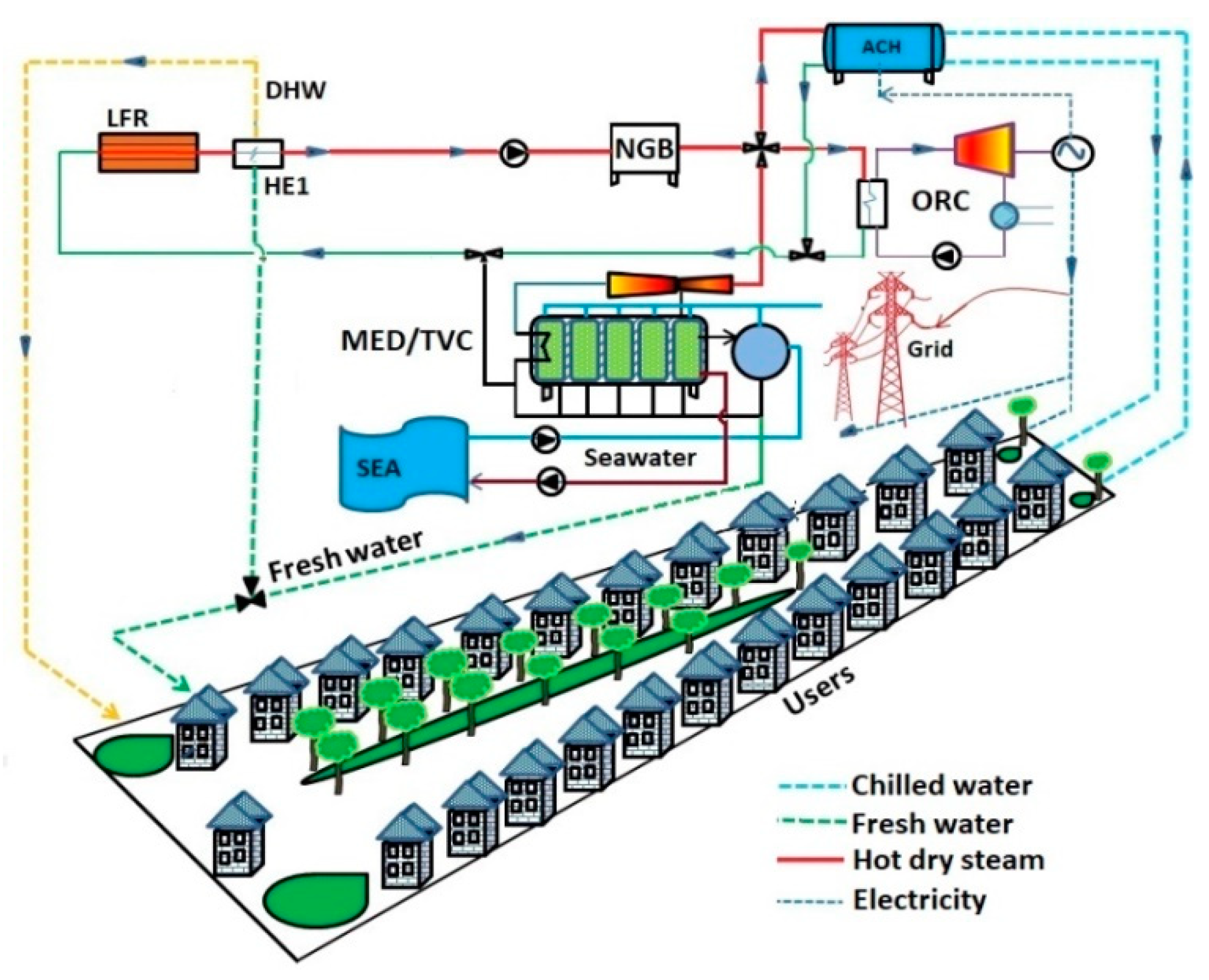
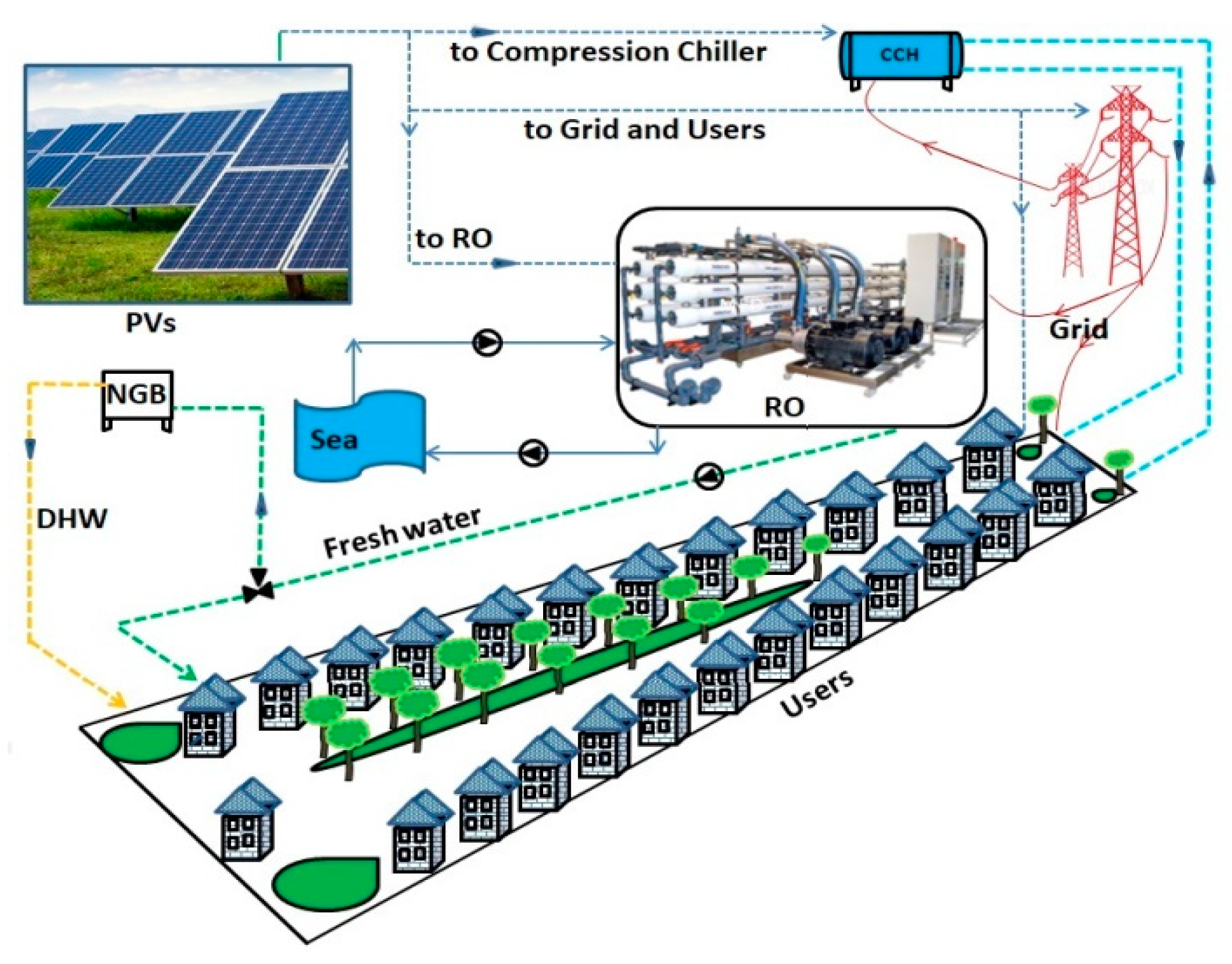
2. System Layout
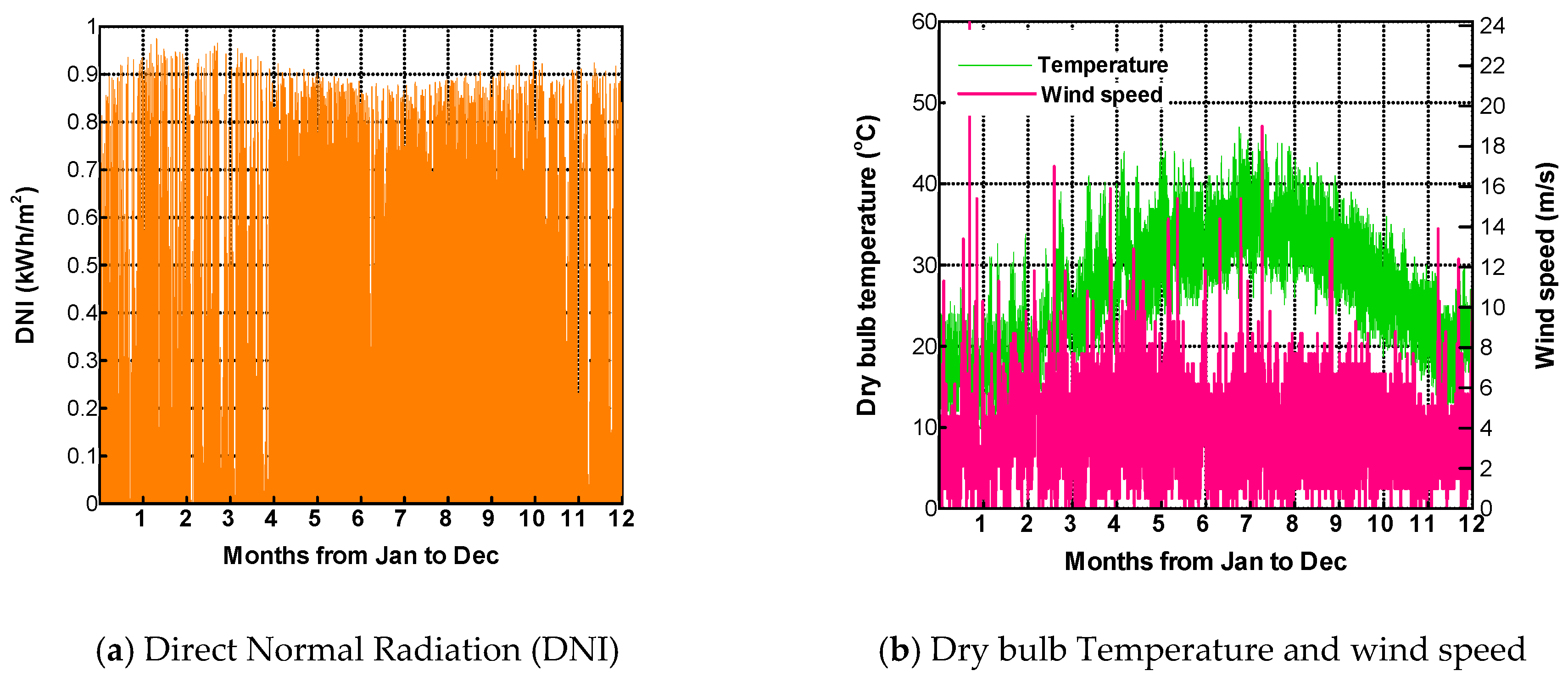
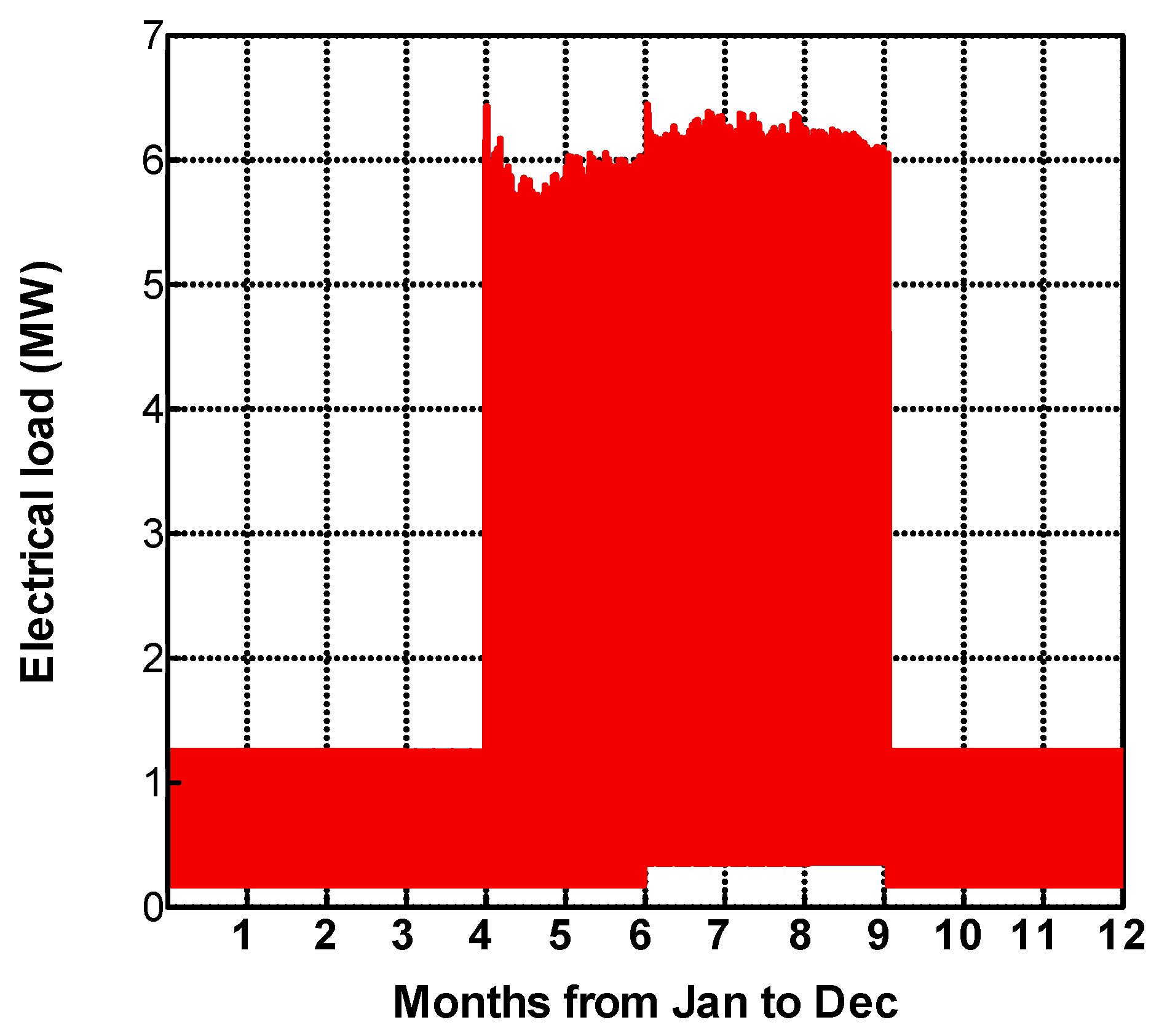
3. Study Area and Building Specifications
4. System Model
- The buildings are modelled through HAP, coupled to the AutoCAD 2018 2D drawing model.
- MED/TVC desalination unit. It is modeled through the MATLAB software and it was validated by the commercial MED/TVC plant which is currently operated on Kish Island located in the Persian Gulf. Please refer to the previous study that has been conducted by some authors of the present study for additional details about the modeling of MED/TVC unit [36].
- The thermodynamic modeling of the ORC was performed using Engineering Equation Solver (EES). Based on the critical temperature of pentane (R601), and its good performance within the temperature ranges of 180 °C to 200 °C, this organic fluid was selected to be used in the ORC.
- The LF solar field and PV plant were modelled using the System Adviser Model (SAM) software provided by U.S. National Renewable Energy Laboratory (NREL) [47].
- The ACH (or CCH) were modelled in EES based on the fixed input thermal energy (or required electricity) and considering the specific chilled water and average seawater cooling temperatures of 7 °C and 30 °C, respectively.
- A simple model was considered for RO desalination unit considering the RO recovery ratio of 45%. For additional details about the modeling of RO unit, please see [36].
4.1. Linear Fresnel Model
4.2. MED/TVC Model
4.3. ORC Model
4.4. Chiller Models
4.5. NGB
4.6. PV Model
4.7. RO Model
5. Economic Analysis
6. Results and Discussion
6.1. Scenatrio#1,
6.1.1. LF Solar Field
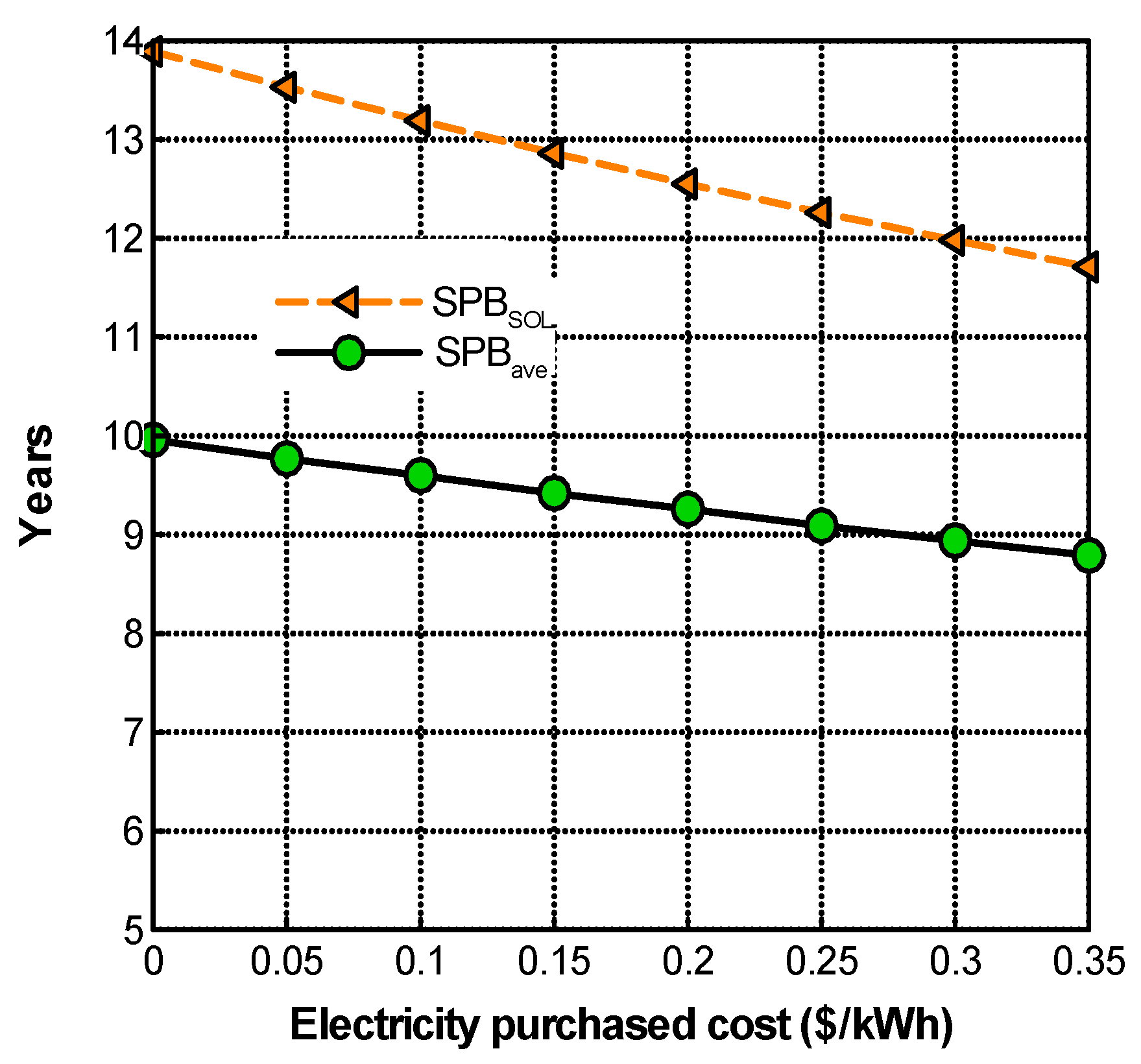
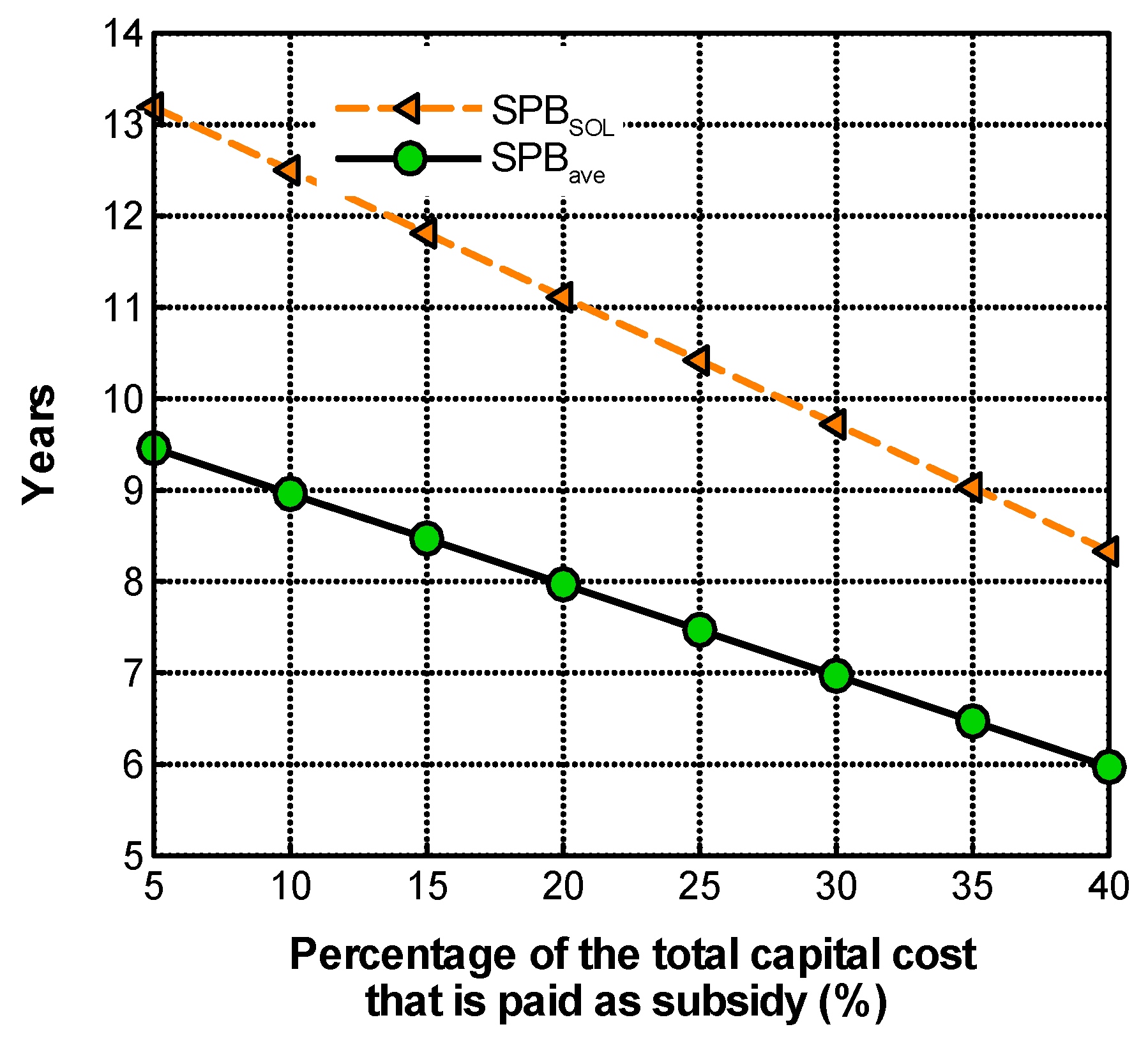
6.1.2. SPB
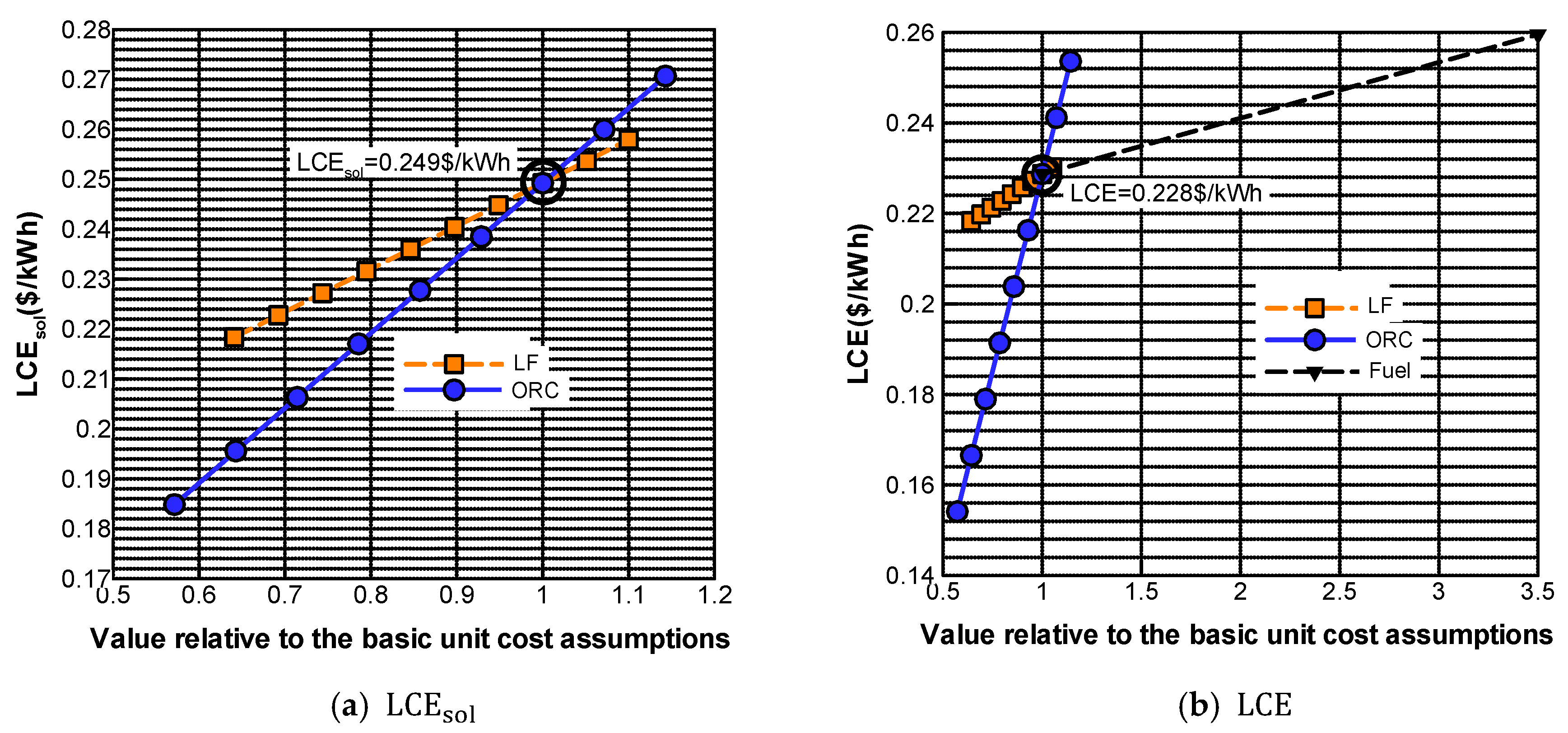
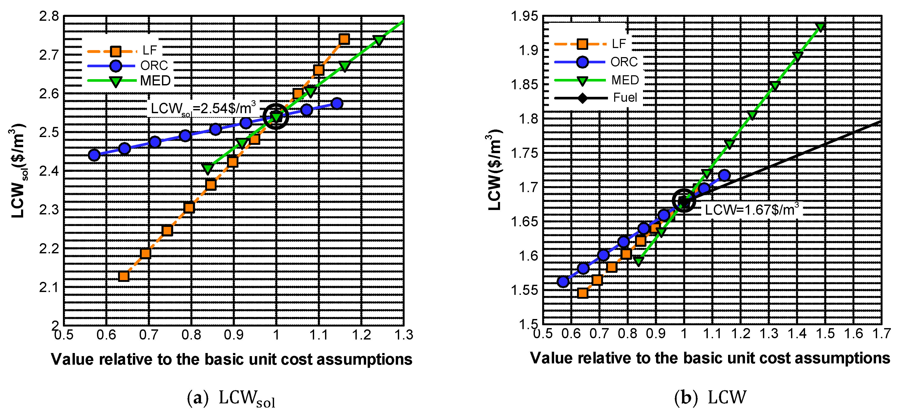
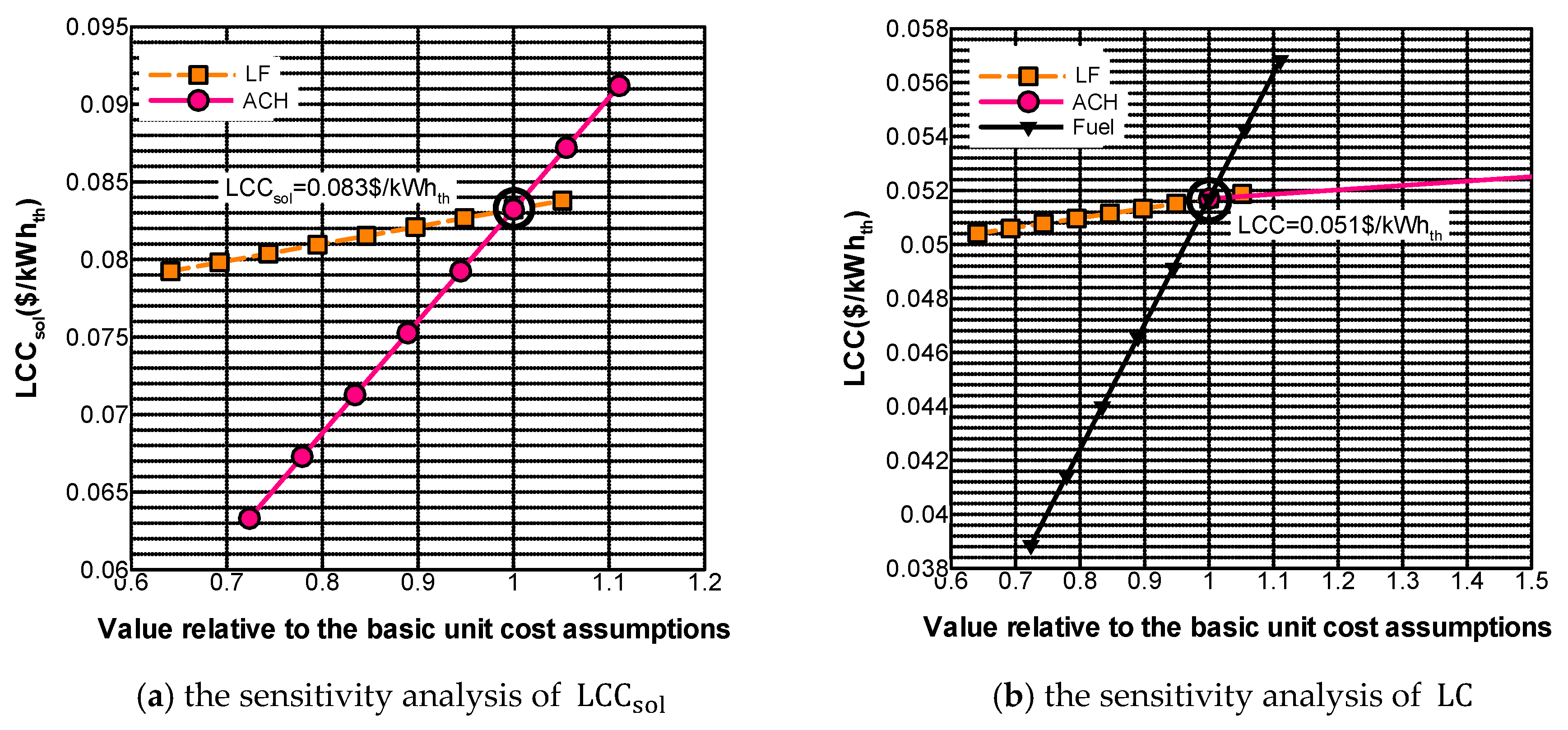
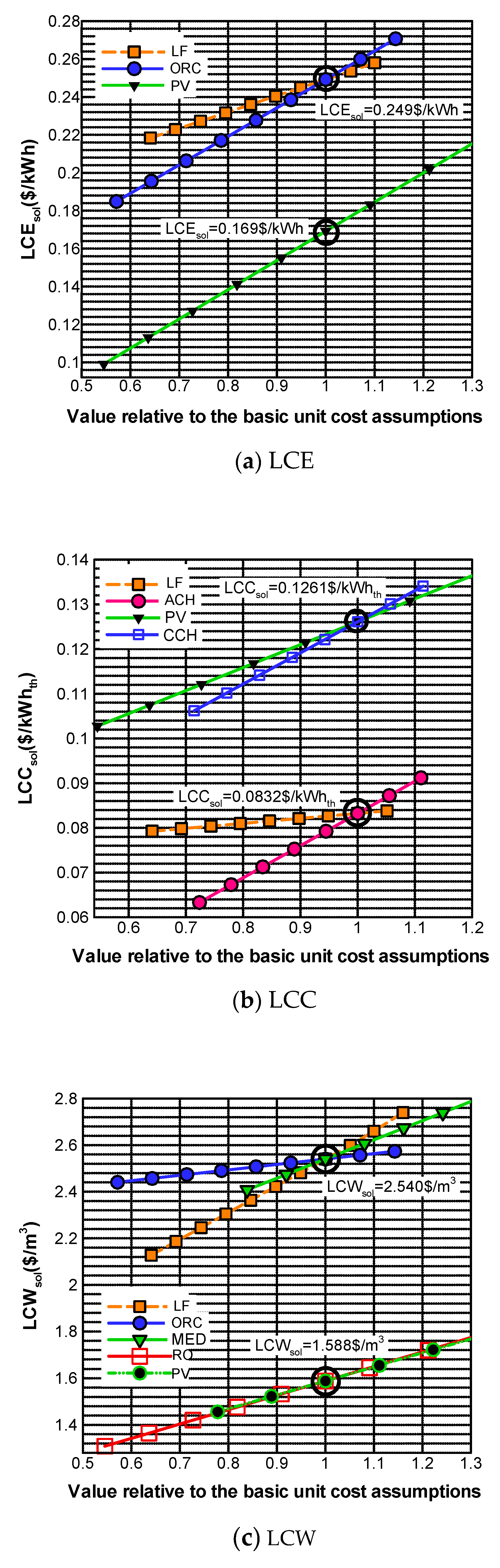
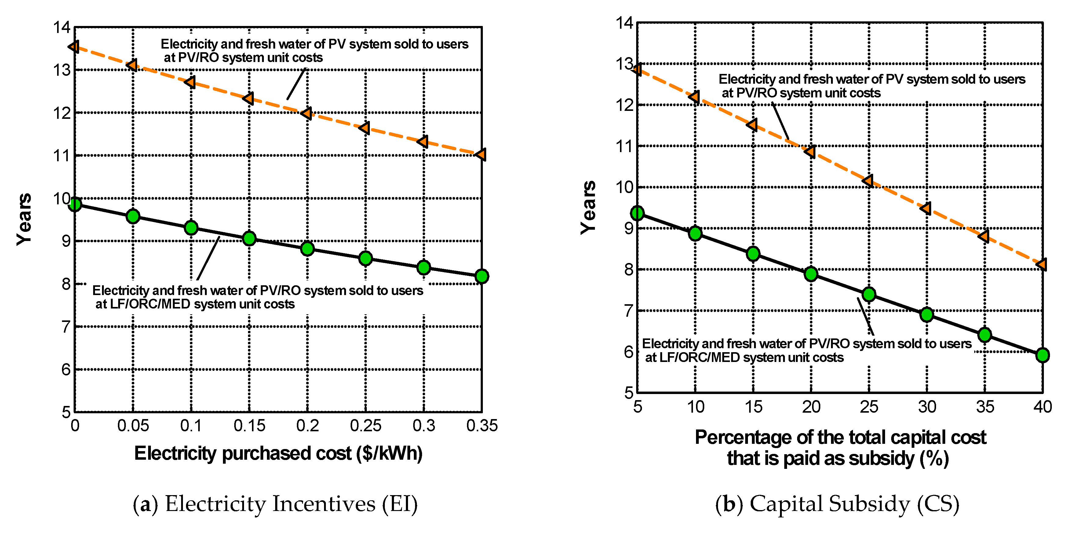
6.1.3. Sensitivity Analysis
6.2. Scenatrio#2
6.2.1. PV Plant
6.2.2. SPB of Scenario#2
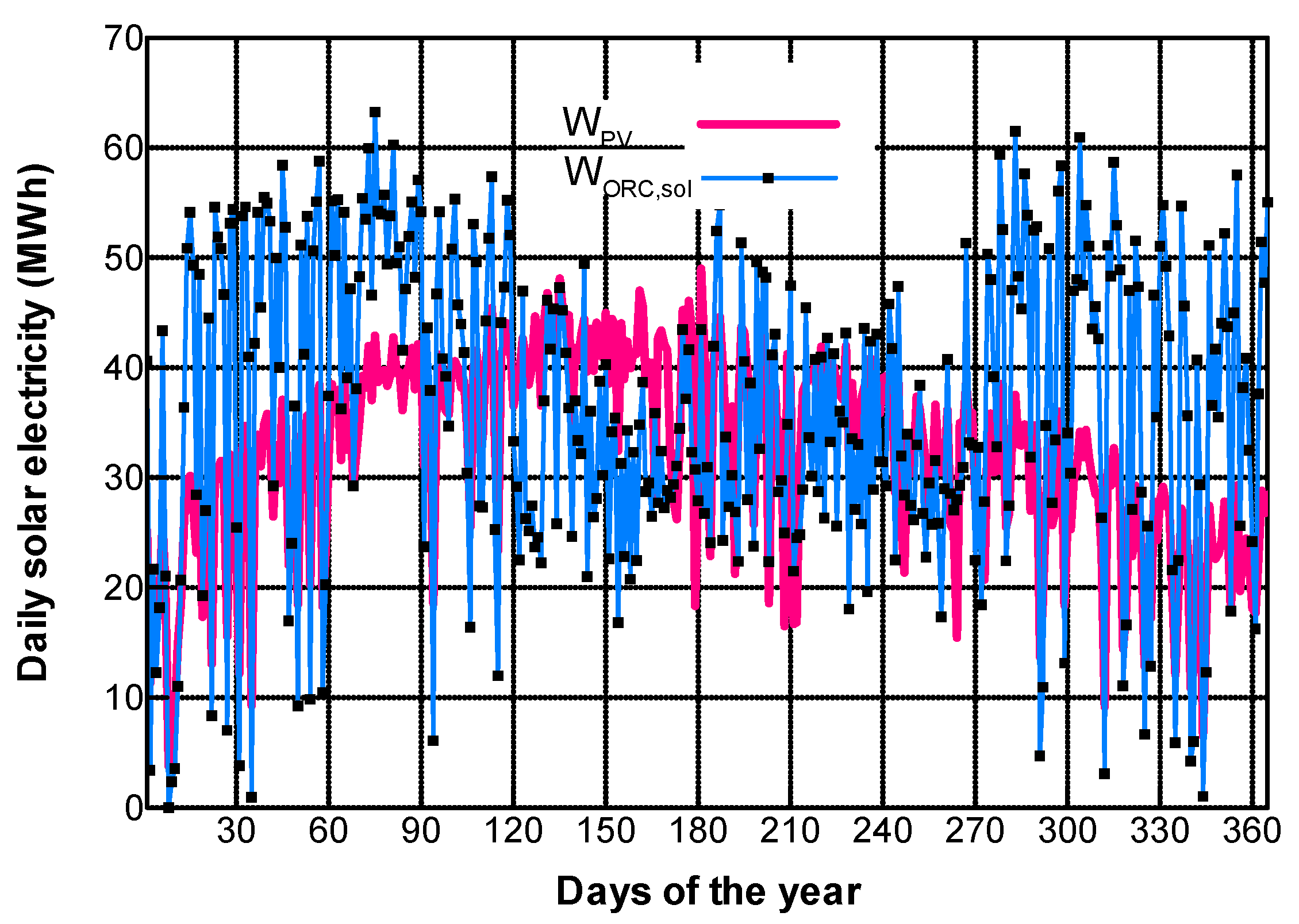
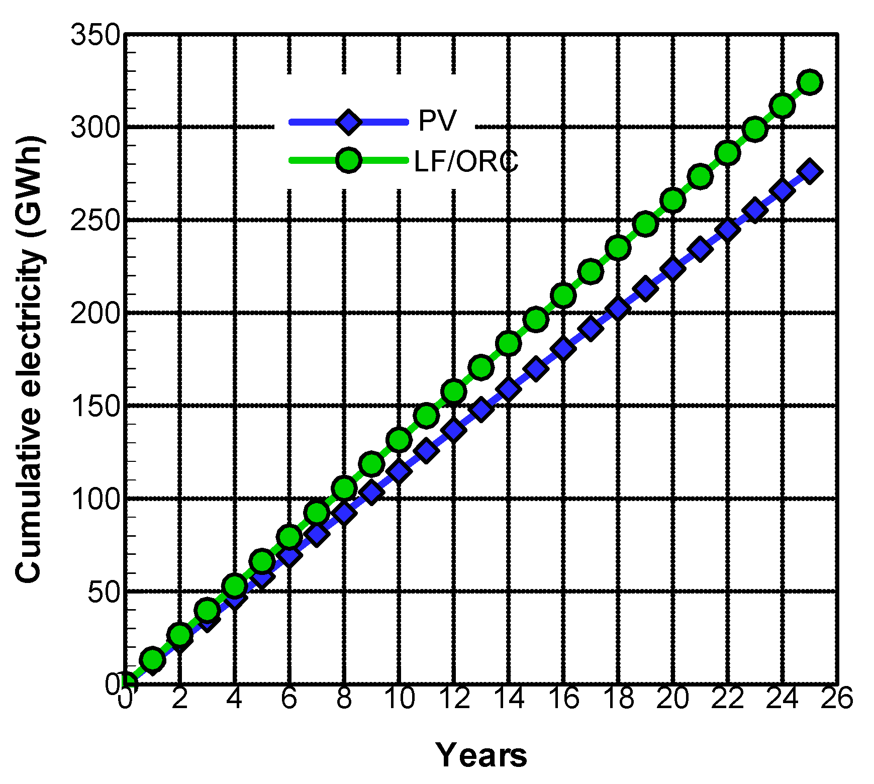
6.3. The Cumulative Electricity Generation
7. Conclusions
Author Contributions
Funding
Conflicts of Interest
Nomenclature
| ACH | Absorption Chiller |
| Solar field aperture area (m2) | |
| LF mirrors aperture area or PV surface area | |
| Total required land area for the solar field | |
| PV module area (m2) | |
| Capital annualized direct costs, $ | |
| Capital annualized indirect costs, $ | |
| Battery | Bat |
| CCH | Compression Chiller |
| CHP | Combined Heat and Power |
| Electricity costs, $ | |
| Fuel costs, $ | |
| Insurance costs, $ | |
| Labor costs, $ | |
| COP | Coefficient of performance |
| CP | Annual cooling production |
| CPC | Compound Parabolic Concentrator |
| CPVT | Concentrated Photovoltaic/Thermal |
| Capital recovery factor | |
| Spare parts replacement costs, $ | |
| Concentrating solar power plant | |
| CUF | Capacity Utilization Factors |
| Direct Normal Irradiation, (W/m2) | |
| DHW | Domestic Hot Water |
| EG | Annual electricity production |
| ETC | Evacuated flat plate solar Collector |
| total electricity that is generated by solar (LF/ORC or PV) | |
| total available solar energy on the solar field | |
| Temperature correction factor | |
| GHI | Global Horizontal Irradiance |
| Gain Output Ratio | |
| HE | Heat exchanger |
| Enthalpy of the steam at the outlet of the solar field | |
| HP | Annual heating production |
| Natural gas heating value | |
| HTF | Heat Transfer Fluid |
| i | Interest rate (%) |
| Transversal incident angle modifier | |
| Longitudinal incident angle modifier | |
| IEA | International Energy Agency |
| Reference total incident radiation, 1000 W/m2 | |
| Total incident global radiation (W/m2) | |
| Receiver length, m | |
| LCE | Levelised cost of electricity, $/kWh |
| LCC | Levelised cost of cooling energy, |
| LCH | Levelised cost of heating energy, |
| LCW | Levelised cost of water, $/m3 |
| Focal distance, m | |
| Linear Fresnel solar field | |
| LF/ORC/ACH/MED configuration | |
| Natural gas mass | |
| Fresh water flow rate | |
| Motive steam mass flow rate | |
| Mass flow rate that is flowed through the ORC heat exchanger | |
| ME | Middle East |
| MED | Multi Effect desalination |
| Number of project Life time | |
| Natural gas boiler | |
| NREL | Natural Renewable Energy Laboratory |
| ORC | Organic Rankine Cycle |
| PEMFC | Proton Exchange Membrane Fuel Cell |
| PTC | Parabolic Trough solar Collector |
| PV | Photovoltaic |
| PV/CCH/RO polygeneration scenario | |
| PVT | Photovoltaic/Thermal |
| Absorbed solar energy, W/m2 | |
| Heat transfer fluid heat loss, W/m2 | |
| Heat lost from solar field pipes, W/m2 | |
| Solar field useful thermal output, W/m2 | |
| Incident thermal power, W/m2 | |
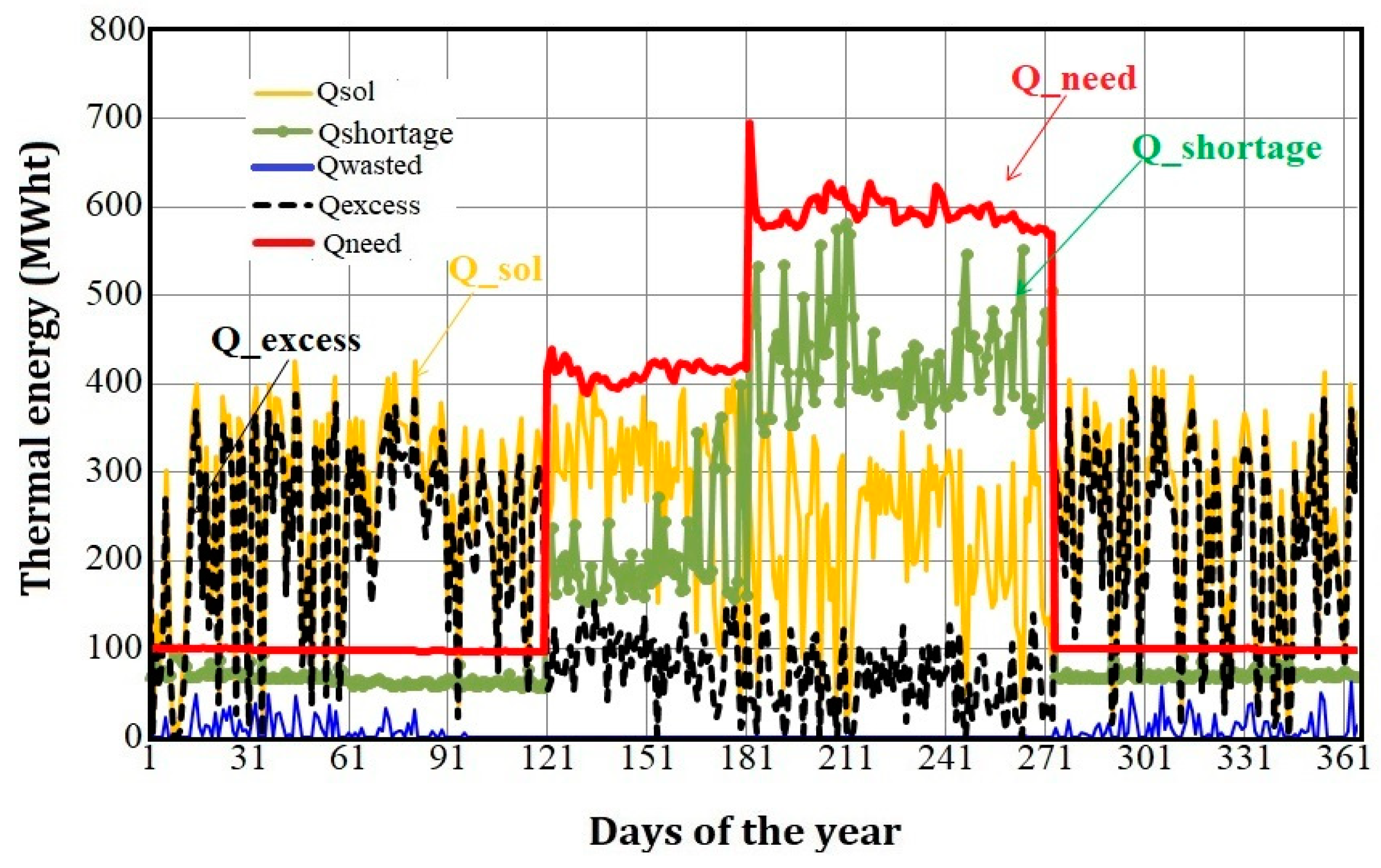
| Hourly LF solar thermal energy that is used to supply the (Qneed(t)) | |
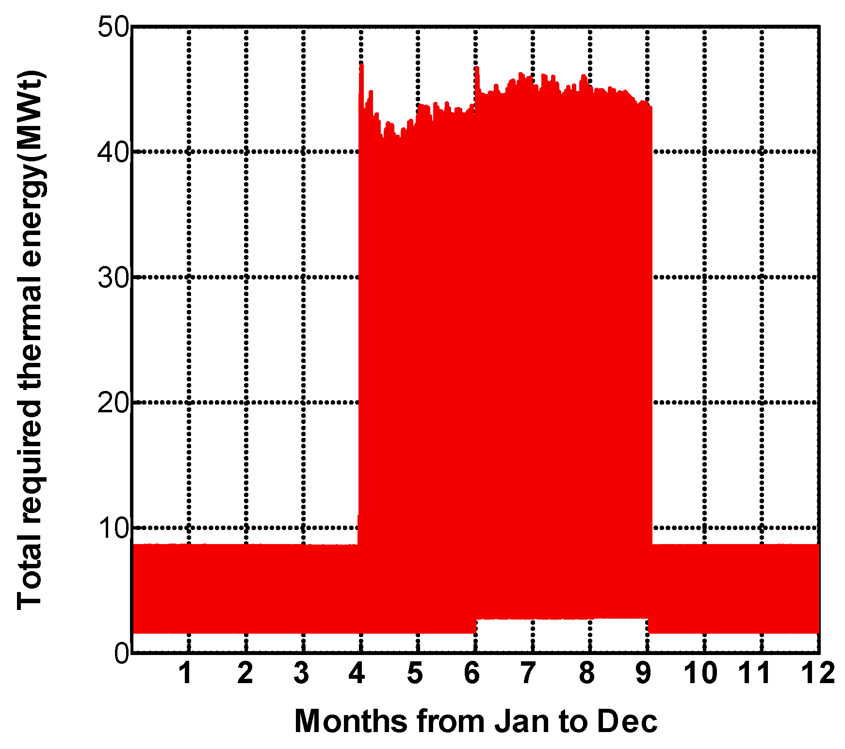
| Hourly required thermal energy of the system | |
| RO | Reverse Osmosis |
| SAM | System Advisor Model |
| SORC | Solar Organic Rankine cycle |
| SRC | Solar Rankine cycle |
| SWRO | Seawater Reverse Osmosis |
| Annual water production, m3/yr | |
| Temperature of the input stream from the sea | |
| Temperature of the output stream to the sea | |
| Thermal energy storage | |
| TVC | Thermal Vapor Compression |
| Greek symbols | |
| Sun elevation angle, degree | |
| Power temperature coefficient | |
| Effectiveness of heat exchanger | |
| End loss efficiency | |
| Optical efficiency | |
| PV module efficiency | |
| The angle of incidence, degree | |
| Zenith angle, degree | |
| Azimuth angle, degree | |
| PV maximum power temperature coefficient | |
| Longitudinal angle, degree | |
| Transversal angle, angle | |
Appendix A

| LCH: | |
| (1a) | |
| (2a) | |
| (3a) | |
| LCC: | |
| (4a) | |
| (5a) | |
| (6a) | |
| LCE: | |
| (7a) | |
| (8a) | |
| (9a) | |
| LCW: | |
| (10a) | |
| (11a) | |
| (12a) | |
| LCH: | |
| (13a) | |
| LCC: | |
| (14a) | |
| LCE: | |
| (15a) | |
| LCW: | |
| (16a) | |
| MED Direct Costs (DC), Indirect Costs (IC) and (O&M) | |
| Main investment ($/m3/day) | 1240 |
| Post-treatment plant ($/m3) | 120 |
| Open sea water intakes ($/m3) | 313 |
| Drinking water storage and pumping ($/m3) | 100 |
| Freight & insurance rate during construction | 5.00% DC |
| Owner’s cost rate | 10.00% of direct material and labor cost |
| Contingency rate | 10.00% of DC |
| Construction overhead (interest during construction) | 12.24% of DC |
| Electricity costs ($/m3) | Depending on Electricity cost (Assuming: 1.55 kWh/m3) |
| Spare parts Replacement | 1.5% of total DC |
| Chemical cost of product water ($/m3) | 0.04 |
| insurance | 0.5% of total DC |
| Natural Gas auxiliary boiler costs ($/m3) | 0.02 to 0.8 |
| Labor cost of product water ($/m3) | 0.025 |
| RO Direct Costs (DC), Indirect Costs (IC) and (O&M) | |
| Main investment ($/m3/day) | 900 |
| Pretreatment plant ($/m3) | 250 |
| Post-treatment plant ($/m3) | 120 |
| Open sea water intakes ($/m3) | 313 |
| Drinking water storage and pumping ($/m3) | 100 |
| Wastewater collection & treatment ($/m3) | 50 |
| Freight & insurance rate during construction | 5.00% DC |
| Owner’s cost rate | 10.00% of direct material and labor cost |
| Contingency rate | 10.00% of DC |
| Construction overhead (interest during construction) | 12.24% of DC |
| Electricity costs ($/m3) | Depending on Electricity cost (Assuming: 3.5 kWh/m3) |
| Spare parts Replacement | 1.5% of total DC |
| Chemical cost of product water ($/m3) | 0.04 |
| insurance | 0.5% of total DC |
| Natural Gas auxiliary boiler costs ($/m3) | 0.02 to 0.8 |
| Labor cost of product water ($/m3) | 0.05 |
| Solar LF Direct Costs (DC) and Indirect Costs (ID) | |
| Site improvement ($/m2) | 20 |
| Solar filed ($/m2) | 150 |
| HTF system ($/m2) | 35 |
| Contingency rate | 7.00% total DC |
| Design and Construction | 15% of total DC |
| Land cost ($/m2) | 10 |
| insurance | 1% of total DC |
| ORC Direct Costs (DC) and Operation (OC) | |
| Direct Costs (DC) | [64] |
| Operation Costs (OC) ($/kWh) | 0.013 |
| PV Direct Costs (DC) and Operation (OC) | |
| Direct Costs ($/kW) | 3300 [65] |
| Operation Costs (OC) ($/kW-year) | 25 |
| ACH Direct Costs (DC) and Operation (OC) | |
| Direct Costs ($/kW) | [23] and [24] |
| Operation Costs (OC) ($/kWh) | 15% of total DC |
| CCH Direct Costs (DC) and Operation (OC) | |
| Direct Costs ($/kW) | 350 [24] |
| Operation Costs (OC) ($/kWh) | 15% of total DC |
| NGB Direct Costs (DC) and Operation (OC) | |
| NGB ($/) | 10 [31] |
| Operation Costs (OC) ($/kWh) | 0.0028 |
References
- IRENA. Renewable Power Generation Costs in 2014. 2015. Available online: https://www.irena.org/documentdownloads/publications/irena_re_power_costs_2014_report.pdf (accessed on 27 August 2019).
- Technology Road Map: Solar Thermal Electricity-2014 Edition, in, International Energy Agency (IEA) Report. 2014. Available online: http://www.solarconcentra.org/wp-content/uploads/2017/06/Technology-Roadmap-Solar-Thermal-Electricity-2014-edition-IEA-1.pdf (accessed on 17 September 2019).
- Technology Road Map: Solar Photovoltaic Energy-2014 Edition, in, International Energy Agency (IEA) Report. 2014. Available online: https://www.iea.org/publications/freepublications/publication/TechnologyRoadmapSolarPhotovoltaicEnergy_2014edition.pdf (accessed on 14 November 2019).
- Observatoire des Energies Renouvelables (ObservER). Worldwide Electricity Production from Renewable Energy Sources. Stats and Figures Series. Thirteenth Inventory. Available online: http://www.energies-renouvelables.org/observ-er/ html/inventaire/Eng/organisation.asp (accessed on 25 September 2019).
- IEA Report. 2016. Available online: http://energyatlas.iea.org/#!/tellmap/1378539487 (accessed on 8 September 2019).
- Baniasad Askari, I.; Oukati Sadegh, M.; Ameri, M. Energy Management and Economics of a Trigeneration System: Considering the Effect of Solar PV, Solar collector and Fuel Price. Energy Sustain. Dev. 2015, 26, 43–55. [Google Scholar] [CrossRef]
- Connolly, D.; Lund, H.; Mathiesen, B.V. Smart Energy Europe: The technical and economic impact of one potential 100% renewable energy scenario for the European Union. Renew. Sustain. Energy Rev. 2016, 60, 1634–1653. [Google Scholar] [CrossRef]
- Calise, F.; Dentice d’Accadia, M.; Libertini, L.; Quiriti, E.; Vicidomini, M. A novel tool for thermoeconomic analysis and optimization of trigeneration systems a case study for a hospital building in Italy. Energy 2017, 126, 64–87. [Google Scholar] [CrossRef]
- Mancarella, P. MES (multi-energy systems): An overview of concepts and evaluation models. Energy 2014, 65, 1–17. [Google Scholar] [CrossRef]
- Kasaeiana, A.; Nouri, G.; Ranjbaran, P.; Wen, D. Solar collectors and photovoltaics as combined heat and power systems: A critical review. Energy Convers. Manag. 2018, 156, 688–705. [Google Scholar] [CrossRef]
- Buonomano, A.; Calise, F.; Palombo, A.; Vicidomini, M. Adsorption chiller operation by recovering low-temperature heat from building integrated photovoltaic thermal collectors: Modelling and simulation. Energy Convers. Manag. 2017, 149, 1019–1036. [Google Scholar] [CrossRef]
- Desai, N.B.; Bandyopadhyay, S. Thermo-economic analysis and selection of working fluid for solar organic Rankine cycle. Appl. Therm. Eng. 2016, 95, 471–481. [Google Scholar] [CrossRef]
- Calise, F.; Dentice d’Accadia, M.; Palombo, A. Exergetic and exergoeconomic analysis of a renewable polygeneration system and viability study for small isolated communities. Energy 2015, 92, 290–307. [Google Scholar] [CrossRef]
- Calise, F.; Dentice d’Accadia, M.; Macaluso, A.; Palombo, A.; Vanoli, L. Exergetic and exergoeconomic analysis of a novel hybrid solar-geothermal polygeneration system producing energy and water. Energy Convers. Manag. 2016, 115, 200–220. [Google Scholar] [CrossRef]
- Tzivanidis, C.; Bellos, E.; Antonopoulos, K.A. Energetic and financial investigation of a stand-alone solar-thermal Organic Rankine Cycle power plant. Energy Convers. Manag. 2016, 126, 421–433. [Google Scholar] [CrossRef]
- Calise, F.; Dentice d’Accadia, M.; Vicidomini, M.; Scarpellino, M. Design and simulation of a prototype of a small-scale solar CHP system based on evacuated flat-plate solar collectors and Organic Rankine Cycle. Energy Convers. Manag. 2015, 90, 347–363. [Google Scholar] [CrossRef]
- Bellos, B.; Tzivanidis, C. Parametric analysis and optimization of an Organic Rankine Cycle with nano fluid based solar parabolic trough collectors. Renew. Energy 2017, 114, 1376–1393. [Google Scholar] [CrossRef]
- Bellos, B.; Tzivanidis, C. Investigation of a hybrid ORC driven by waste heat and solar energy. Energy Convers. Manag. 2018, 156, 427–439. [Google Scholar] [CrossRef]
- Garcia-Saez, I.; Méndez, J.; Ortiz, C.; Loncar, D.; Becerra, J.A.; Chacartegui, R. Energy and economic assessment of solar Organic Rankine Cycle for combined heat and power generation in residential applications. Renew. Energy 2019, 140, 461–476. [Google Scholar] [CrossRef]
- Mazloumi, M.; Naghashzadegan, M.; Javaherdeh, K. Simulation of solar lithium bromide–water absorption cooling system with parabolic trough collector. Energy Convers. Manag. 2008, 49, 2820–2832. [Google Scholar] [CrossRef]
- Chahartaghi, M.; Golmohammadi, H.; Faghih Shojaei, A. Performance analysis and optimization of new double effect lithium bromide-water absorption chiller with series and parallel flows. Int. J. Refrig. 2019, 97, 73–87. [Google Scholar] [CrossRef]
- Delač, B.; Pavković, B.; Lenić, K. Design, Monitoring and dynamic model development of a solar heating and cooling system. Appl. Therm. Eng. 2018, 142, 489–501. [Google Scholar] [CrossRef]
- Bellos, B.; Tzivanidis, C. Energetic and financial analysis of solar cooling systems with single effect absorption chiller in various climates. Appl. Therm. Eng. 2017, 126, 809–821. [Google Scholar] [CrossRef]
- Calise, F.; Dentice d’Accadia, M.; Libertini, L.; Quiriti, E.; Vanoli, R.; Vicidomini, M. Optimal operating strategies of combined cooling, heating and power systems: A case study for an engine manufacturing facility. Energy Convers. Manag. 2017, 149, 1066–1084. [Google Scholar] [CrossRef]
- Shirazi, A.; Taylor, R.A.; Morrisona, G.L.; White, S.D. Solar-powered absorption chillers: A comprehensive and critical review. Energy Convers. Manag. 2018, 171, 59–81. [Google Scholar] [CrossRef]
- Buonomano, A.; Calise, F.; Palombo, A. Solar heating and cooling systems by absorption and adsorption chillers driven by stationary and concentrating photovoltaic/thermal solar collectors: Modelling and simulation. Renew. Sustain. Energy Rev. 2018, 82, 1874–1908. [Google Scholar] [CrossRef]
- Bellos, B.; Tzivanidis, C. Parametric analysis and optimization of a solar driven trigeneration system based on ORC and absorption heat pump. J. Clean. Prod. 2017, 161, 493–509. [Google Scholar] [CrossRef]
- Xu, Z.Y.; Wang, R.Z. Comparison of CPC driven solar absorption cooling systems with single, double and variable effect absorption chillers. Sol. Energy 2017, 158, 511–519. [Google Scholar] [CrossRef]
- Akrami, E.; Nemati, A.; Nami, H.; Ranjbar, F. Exergy and exergo economic assessment of hydrogen and cooling production from concentrated PVT equipped with PEM electrolyzer and LiBr-H2O absorption chiller. Int. J. Hydrog. Energy 2018, 43, 622–633. [Google Scholar] [CrossRef]
- Shekarchiana, M.; Moghavvemib, M.; Motasemi, F.; Mahlia, T.M.I. Energy savings and cost–benefit analysis of using compression and absorption chillers for air conditioners in Iran. Renew. Sustain. Energy Rev. 2011, 15, 1950–1960. [Google Scholar] [CrossRef]
- Ghafurian, M.M.; Niazmand, H. New approach for estimating the cooling capacity of the absorption and compression chillers in a trigeneration system. Int. J. Refrig. 2018, 86, 89–106. [Google Scholar] [CrossRef]
- Calise, F.; Damian Figaj, R.; Massarotti, N.; Mauro, A.; Vanoli, L. Polygeneration system based on PEMFC, CPVT and electrolyzer: Dynamic simulation and energetic and economic analysis. Appl. Energy 2017, 192, 530–542. [Google Scholar] [CrossRef]
- Leiva-Illanes, R.; Escobar, R.; Cardemil, J.M.; Alarcón-Padillad, D.C. Thermo economic assessment of a solar polygeneration plant for electricity, water, cooling and heating in high direct normal irradiation conditions. Energy Convers. Manag. 2017, 151, 538–552. [Google Scholar] [CrossRef]
- Baneshi, M.; Hadianfard, F. Techno-economic feasibility of hybrid diesel/PV/wind/battery electricity generation systems for non-residential large electricity consumers under southern Iran climate conditions. Energy Convers. Manag. 2016, 127, 233–244. [Google Scholar] [CrossRef]
- Baniasad Askari, I.; Ameri, M. Combined linear Fresnel solar Rankine cycle with multi-effect desalination (MED) process: Effect of solar DNI level on the electricity and water production costs. Desalin. Water Treat. 2018, 126, 97–115. [Google Scholar] [CrossRef]
- Baniasad Askari, I.; Ameri, M.; Calise, F. Energy, exergy and exergo-economic analysis of different water desalination technologies powered by Linear Fresnel solar field. Desalination 2018, 428, 37–67. [Google Scholar] [CrossRef]
- Baniasad Askari, I.; Ameri, M. The application of Linear Fresnel and Parabolic Trough solar fields as thermal source to produce electricity and fresh water. Desalination 2017, 415, 90–103. [Google Scholar] [CrossRef]
- Bellos, B.; Tzivanidis, C.; Moschos, K.; Antonopoulos, K.A. Energetic and financial evaluation of solar assisted heat pump space heating systems. Energy Convers. Manag. 2016, 120, 306–319. [Google Scholar] [CrossRef]
- Baccioli, A.; Antonelli, M.; Desideri, U.; Grossi, A. Thermodynamic and economic analysis of the integration of Organic Rankine Cycle and Multi-Effect Distillation in waste-heat recovery applications. Energy 2018, 161, 456–469. [Google Scholar] [CrossRef]
- Baniasad Askari, I.; Ameri, M. Techno Economic Feasibility Analysis of MED/TVC Desalination Unit Powered by Linear Fresnel Solar Field Direct Steam. Desalination 2016, 394, 1–17. [Google Scholar] [CrossRef]
- Baniasad Askari, I.; Ameri, M. Solar Rankin Cycle (SRC) Powered by Linear Fresnel Solar Field and Integrated With Combined MED Desalination system. Renew. Energy 2018, 117, 52–70. [Google Scholar] [CrossRef]
- Fichtner (Fichtner GmbH&Co. KG) and DLR (Deutsches Zentrum für Luft und Raumfahrt e.V.), MENA Regional Water Outlook, Part II, Desalination Using Renewable Energy, Task 1—Desalination Potential. 2011. Available online: http://www.dlr.de/tt/Portaldata/41/Resources/dokumente/institut/system/projects/MENA_REGIONAL_WATER_ OUTLOOK.pdf (accessed on 2 November 2019).
- Javadpour, A.; Jahanshahi Javaran, E.; Lari, K.; Baniasad Askari, I. Techno-economic analysis of combined gas turbine, MED and RO desalination systems to produce electricity and drinkable water. Desalin. Water Treat. 2019, 159, 232–249. [Google Scholar] [CrossRef] [Green Version]
- Patil, V.R.; Biradar, V.I.; Shreyas, R.; Garg, P.; Orosz, M.S.; Thirumalai, N.C. Techno-economic comparison of solar organic Rankine cycle (ORC) and photovoltaic (PV) systems with energy storage. Renew. Energy 2017, 113, 1250–1260. [Google Scholar] [CrossRef]
- Awana, A.B.; Zubair, M.; Praveen, R.P.; Bhatti, A.R. Design and comparative analysis of photovoltaic and parabolic trough based CSP plants. Sol. Energy 2019, 183, 551–565. [Google Scholar] [CrossRef]
- Desideri, U.; Campana, P.E. Analysis and comparison between a concentrating solar And a photovoltaic power plant. Appl. Energy 2014, 113, 422–433. [Google Scholar] [CrossRef]
- System Adviser Model (SAM), Version 2015.6.30. Available online: https://www.nrel.gov/analysis/ sam/help/html-php/index.html?linear_fresnel_system_costs.htm (accessed on 5 October 2019).
- Kelly, B.; Kearney, D. Parabolic Trough Solar System Piping Model Final Report, National Renewable Energy Laboratory Subcontract Report NREL/SR-550-40165, July 2006. Available online: Available electronically at http://www.nrel.gov/csp/troughnet/pdfs/40165.pdf (accessed on 10 October 2019).
- PTR70 Parabolic Trough Receiver, National Renewable Energy Laboratory, Technical Report No. NREL/TP-550–45633. Available online: https://www.nrel.gov/docs/fy09osti/45633.pdf (accessed on 5 November 2019).
- Kouhikamali, R. Thermodynamic analysis of feed water pre-heaters in multiple effect distillation systems. Appl. Therm. Eng. 2013, 50, 1157–1163. [Google Scholar] [CrossRef]
- Persian Gulf Seawater Salinity. Available online: http://www7320.nrlssc.navy.mil/global_ncom/glb8_3b/html/pgulf.html (accessed on 10 November 2019).
- Persian Gulf seawater salinity. Available online: http://havajanah.ir/?page_id=924 (accessed on 8 November 2019).
- Calise, F.; Dentice d’Accadia, M.; Piacentino, A. A novel solar trigeneration system integrating PVT (photovoltaic/thermal collectors) and SW (seawater) desalination: Dynamic simulation and economic assessment. Energy 2014, 67, 129–148. [Google Scholar] [CrossRef]
- Yu, H.; Gundersen, T.; Feng, X. Process integration of organic Rankine cycle (ORC) and heat pump for low temperature waste heat recovery. Energy 2018, 160, 330–340. [Google Scholar] [CrossRef]
- Zheng, X.; Shi, R.; Wang, Y.; You, S.; Zhang, H.; Xia, J.; Wei, S. Mathematical modeling and performance analysis of an integrated solar heating and cooling system driven by parabolic trough collector and double-effect absorption chiller. Energy Build. 2019, 202. [Google Scholar] [CrossRef]
- Underwood, C.P. Advances in Ground-Source Heat Pump Systems, 1st ed.; Woodhead: Cambridge, UK, 2016; pp. 387–421. [Google Scholar]
- Baniasad Askari, I.; Ameri, M. The Effect of fuel price on economic analysis of hybrid (photovoltaic/diesel/battery) systems in Iran. Energy Sources Part B Econ. Plan. Policy 2011, 11, 357–377. [Google Scholar] [CrossRef]
- Baniasad Askari, I.; Oukati Sadegh, M.; Ameri, M. Effect of heat storage and fuel price on energy management and economics of micro CCHP cogeneration systems. J. Mech. Sci. Technol. 2014, 28, 2003–2014. [Google Scholar] [CrossRef]
- Baniasad Askari, I.; Ameri, M. Optimal sizing of photovoltaic-battery power systems in a remote region in Kerman, Iran. Proc. Inst. Mech. Eng. Part A J. Power and Energy 2009, 223, 563–570. [Google Scholar] [CrossRef]
- Duffie, J.; Beckman, W. Solar Engineering of Thermal Processes, 2nd ed.; ASME: Hoboken, NJ, USA, 2006. [Google Scholar]
- Palenzuela, P.; Zaragoza, G.; Alarcon-Padilla, D.C. Characterisation of the coupling of multi-effect distillation plants to concentrating solar power plants. Energy 2015, 82, 986–995. [Google Scholar] [CrossRef]
- Loutatidou, S.; Arafat, H.A. Techno-economic analysis of MED and RO desalination powered by low enthalpy geothermal energy. Desalination 2015, 365, 277–292. [Google Scholar] [CrossRef]
- Electricity Incentive Policy in Iran. Available online: http://electricity%20and%20gas%20prices/Iran%20Solar%20Brochure.pdf (accessed on 12 November 2019).
- Eveloy, V.; Rodgers, P.; Qiu, L. Hybrid gas turbine–organic Rankine cycle for seawater desalination by reverse osmosis in a hydro carbon production facility. Energy Convers. Manag. 2015, 106, 1134–1148. [Google Scholar] [CrossRef]
- Khosravi, A.; Syri, S.; Assad, M.E.H.; Malekan, M. Thermodynamic and Economic analysis of a hybrid ocean thermal energy conversion/photovoltaic system with hydrogen-based energy storage system. Energy 2019, 172, 304–319. [Google Scholar] [CrossRef]


| Ref. | Technology/Temperature | Modelling/Review | Results | Applications |
|---|---|---|---|---|
| [10] | PVT and CPVT | Review | Please refer to paper | Electricity and heating |
| [11] | PVT/ACH/Bat/NGB (50–60 °C) | Energy, economic, environmental | System payback time: 10.6–11.3 years | Electricity, space heating and cooling |
| [12] | PTC/ORC and LF/ORC (Up to 400 °C) | Techno-economic assessment | PTC/ORC: 0.344–0.476 $/kWh, LF/ORC: 0.353–0.488 $/kWh | Electricity |
| [13] | CPVT/Biomass/ACH/MED (90 °C) | Exergetic and exergo-economic analysis | Electricity: 0.042–0.268 Heating: 0.007– 0.077 Cooling: 0.008– 0.086 Fresh water: 1.7– 8 | Electricity, space heating, cooling and fresh water |
| [14] | PTC/Geothermal/ACH/MED (160–200 °C) | Exergo-economic analysis | Electricity: 0.1475–0.1722 €/kWh, Cooling: 0.5695–0.6023 Fresh water: 0.431–0.458. | Electricity, space heating, cooling and fresh water |
| [15] | PTC/ORC (235–300 °C) | Energy and economic | ORC efficiency: 19.57–25.36% System Payback time: 9 years | Electricity: 1 MW |
| [16] | ETC/ORC (230 °C) | Energy and economic | ORC efficiency: 10% System Payback time: 10 years | Electricity: 6 kW |
| [17] | PTC/ORC nanoparticles with thermal oil (300 °C) | Technical Model | System efficiency = 20.11% and is improved by 1.75% using the Nano fluid in the ORC | Electricity: 167 kW |
| [18] | Waste heat/PTC/ORC (150–300 °C) | Technical Model | System efficiency from 11.6–19.7% | Electricity: 479–845 kW |
| [19] | EFPC 2/ORC and EFPC/HP 3 (80–170 °C) | Energy and economic | System Payback: EFPC/ORC: 3.8 years EFPC/HP: 3.1 years | Electricity and heating |
| [20] | PTC/ACH Single effect (90 °C) | Technical modeling | ACH COP: 0.66–0.76 | Cooling: 17.5 kW |
| [21] | ACH (double effect parallel and series flows LiBr/) (145–185 °C) | Technical modeling | ACH COP: 0.45–1.35 | The effects of generator and inlet vapor on COP |
| [22] | ETC/ACH (60–95 °C) | Techno economic assessment | Cooling energy cost: 0.0225 | Cooling capacity: 900 kWh |
| [23] | ETC/ACH (single effect LiBr/) (Up to 90 °C) | Energy and economic analysis | Cooling energy: Abu Dhabi: 0.0575, Rome: 0.2125, Madrid: 0.1792 Thessaloniki: 0.1771 | Cooling in a building with 100 floor area |
| [24] | Waste heat/ACH/CCH/NGB (70–95 °C) | Thermo-economic | System Payback: 3.8–4.8 years COP: 0.7–0.8 | Electricity, space heating, cooling |
| [25] | Solar-assisted/ACH (single and multi-effect) (70–240 °C | Review | Solar ACHs cannot compete economically with conventional cooling without government subsidies | Cooling |
| [26] | CPVT/ACH or PVT/ACH (80–95 °C) | Modelling, review | System Payback: CPVT/ACH (6.1–6.9 years), PVT/ACH (21–29 years) | Electricity, heating, cooling |
| [27] | PTC/ORC/ACH Single effect, LiBr/ (235–360 °C) | Energy, exergy and economic | ACH COP: 0.57–0.85 Second law efficiency: 21.92–29.42% | Electricity and cooling |
| [28] | CPC 4/ACH/TES 5 single, double and variable effect LiBr/ (90–160 °C) | Energy, Simulation | Average COP: 0.7–1.2 Solar efficiency: 10–24% Storage tank volume has an important effect on variable and double effect ACHs | Cooling |
| [29] | CPVT 6/ACH/PEM 7/electrolyzer (100 °C) | Energy–exergy | Cooling: 0.0649 | Cooling and hydrogen |
| [30] | ACH and CCH | Energy, economic | ACH energy demand > CCH energy demand ACH energy cost < CCH energy cost | Cooling |
| [31] | Prime mover/NGB 8/ACH and CCH | four-E analysis (energy, exergy, economy) | System Payback: 5.1 years Exergy efficiency of ACH: 41.9% for grid on mode and 32.7% for grid off mode | Electricity, heating and cooling (900–5600 kW) |
| [32] | CPVT/ACH/PEM Fuel Cell (50–90 °C) | Energy economic | The results are in terms of: Payback time, energy and economic efficiencies and utilization factor | heating, cooling, DHW electricity, hydrogen, oxygen |
| [33] | PTC/SRC 9/ACH/MED/TES/process heat (373 °C) | energy- economic | Electricity: 0.1058–0.1220, Heating: 0.0180.03, Cooling: 0.036–0.055, fresh water: 2.746–4.035 | Electricity, heating, cooling, fresh water |
| [34] | Diesel/PV/Wind/Bat | Techno-economic | Electricity: Off-grid systems = 9.3–12.6 /kWh On-grid/Bat system = 5.7–8.4 /kWh | Electricity |
| [35] | LF/SRC/MED (395 °C) | Techno-economic | Electricity: 0.15–0.23, fresh water: 1.42–1.78 | Electricity and heating |
| [36] | LF/SRC/MED and LF/SRC/RO (373 °C) | Exergo-economic | Electricity: 0.15–0.20 $/kWh, Fresh water: 1.42–2.38 | Electricity and fresh water |
| [37] | LF/SRC/MED and LF/SRC/RO (384 °C) | Techno-economic | For TES = 7.5 h: Electricity and fresh water: 0.19 $/kWh and 1.66 for LF/SRC/MED And 0.23 $/kWh 1.84 for PTC/SRC/MED | Electricity and fresh water |
| [38] | PV/Air source HP, PV/FPC/Water source HP and PVT/FPC/Water source HP (70 °C) | Energy and economic | PV/Air source heat pump is more suitable than PVT/FPC/Water source heat pump if the electricity cost would be up to 0.23 €/kWh | Space heating |
| [39] | Waste heat/ORC/MED (200 °C) | Thermo-economic | Electricity: 0.04–0.12 $/kWh and Fresh water:0.8–1.8 for production capacities of 500–2000 | Electricity and fresh water |
| [40] | LF/MED/TVC/TES (256–520 °C) | Techno- economic | Fresh water: 1.63–3.32 for fresh water rate of 9000 | Fresh water |
| [41] | LF/SRC/MED (390 °C) | Techno-economic | Electricity: 0.16–0.23 $/kWh and Fresh water: 1.85–2.21 for production capacities of 100,000 | Electricity and fresh water |
| [42] | PTC/SRC/MED PTC/SRC/RO (377 °C) | Techno-economic | Electricity: 0.21–0.24 $/kWh and Fresh water: 1.82–2.11 for 100,000 | Electricity and fresh water |
| [43] | GT/MED/TVC/RO (120–354 °C) | Techno-economic | Electricity: 0.018–0.02 $/kWh and Fresh water: 0.5–0.7 for 2000–5000 | Electricity and fresh water |
| Inlet chilled water rated temperature | 12 °C |
| Chilled water set-point temperature | 7 °C |
| Inlet cooling water rated temperature | 30 °C |
| Outlet cooling water rated temperature | 35 °C |
| Inlet hot water rated temperature for ACH operation | 180 °C |
| Outlet hot water rated temperature for ACH operation | 70 °C |
| Chilled water flowrate (pump P3) | 359 kg/s |
| Cooling water flow rate (pump P2) | 780 kg/s |
| Hot water flow rate (pump P1) | 2.64 kg/s |
| COP | 1.2 |
| Rated cooling capacity | 7500 kW |
| Rated Heat Input | 6250 kW |
| 0.013 | 0.003 | 0.006 | 0.083 | 0.037 | 0.051 | 0.249 | 0.228 | 0.218 | 2.540 | 1.268 | 1.67 |
| Solar Field | ORC | Fuel | ACH | MED | |||||
|---|---|---|---|---|---|---|---|---|---|
| Cost ($/m2) | Value | Cost ($/kW) | Value | Cost ($/m3) | Value | Value | Cost ($/m3) | Value | |
| 125 | 0.64 | 2000 | 0.57 | 0.03 | 1.00 | 262 | 0.72 | 1040 | 0.84 |
| 135 | 0.69 | 2250 | 0.64 | 0.105 | 3.50 | 282 | 0.78 | 1140 | 0.92 |
| 145 | 0.74 | 2500 | 0.71 | 0.21 | 7.00 | 302 | 0.83 | 1240 | 1.00 |
| 155 | 0.79 | 2750 | 0.79 | ------ | ------ | 322 | 0.89 | 1340 | 1.08 |
| 165 | 0.85 | 3000 | 0.86 | ------ | ------ | 342 | 0.94 | 1440 | 1.16 |
| 175 | 0.90 | 3250 | 0.93 | ------ | ------ | 362 | 1.00 | 1540 | 1.24 |
| 185 | 0.95 | 3500 | 1.00 | ------ | ------ | 382 | 1.06 | 1640 | 1.32 |
| 195 | 1.00 | 3750 | 1.07 | ------ | ------ | 402 | 1.11 | 1740 | 1.40 |
| 205 | 1.05 | 4000 | 1.14 | ------ | ------ | ------ | ------ | 1840 | 1.48 |
| Parameter | Khormaksar | Masirah | Bandar-Abbas | Bushehr |
|---|---|---|---|---|
| Latitude & Longitude | ||||
| GHI (kWh/m2/year) | 2186 | 1879 | 1858 | 1718 |
| DNI (kWh/m2/year) | 1933 | 1514 | 1462 | 1350 |
| NGB rated capacity (MW) | 51.23 | 51.23 | 51.23 | 51.23 |
| ORC rated power (MW) | 6.50 | 6.50 | 6.50 | 6.50 |
| Natural gas price ($/m3) | 0.03 | 0.03 | 0.03 | 0.03 |
| ACH cooling capacity () | 7.5 | 7.5 | 7.5 | 7.5 |
| MED capacity (m3/day) | 200 | 200 | 200 | 200 |
| Project life time (years) | 25 | 25 | 25 | 25 |
| LF mass flow rate (kg/s) | 25.73 | 25.73 | 25.73 | 25.73 |
| LF output Temperature ( °C) | 185 | 185 | 185 | 185 |
| DNI (kWh/m2/year) | 1933 | 1514 | 1462 | 1350 |
| Solar field area (km2) | 0.057 | 0.057 | 0.060 | 0.060 |
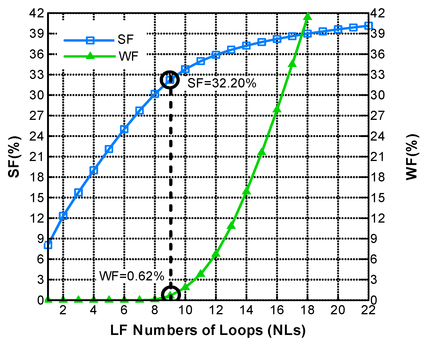
| SF (%) | 32.11 | 28.43 | 32.20 | 28.34 |
| WF (%) | 0.86 | 0.56 | 0.64 | 1.00 |
| 0.010 | 0.0128 | 0.0133 | 0.0144 | |
| 0.0052 | 0.0057 | 0.0063 | 0.0062 | |
| 0.0807 | 0.0924 | 0.0832 | 0.0940 | |
| 0.0508 | 0.0514 | 0.0517 | 0.0516 | |
| 0.1997 | 0.2457 | 0.2492 | 0.2558 | |
| 0.2168 | 0.2325 | 0.2186 | 0.2370 | |
| 2.212 | 2.605 | 2.540 | 2.748 | |
| 1.578 | 1.643 | 1.678 | 1.685 | |
| Total fuel saving () | 3.22 | 2.85 | 3.22 | 2.84 |
| Total CO2 emissions ( tons/yr) | 11.87 | 12.51 | 11.85 | 12.53 |
| Total capital cost (M$) | 38.97 | 38.97 | 40.57 | 40.57 |
| Parameter | Value |
|---|---|
| Nominal efficiency | 15% |
| Max Power | 270.3 W |
| Module length/width | 1.66 m/1 m |
| Max power voltage/Max power current | 31.8 V/8.5 A |
| Open Circuit Voltage/Short Circuit Current | 38.5 V/9 A |
| Temperature Coefficient of Power () | −0.454/ °C |
| Nameplate capacity of the plant | 6500 kW |
| Number of PV modules | 24,074 |
| Inverter Total capacity | 5416 kW |
| Location | Khormaksar | Masirah | Bandar-Abbas | Bushehr | ||||
|---|---|---|---|---|---|---|---|---|
| SF (%) | 32.11 | 28.43 | 32.20 | 28.34 | ||||
| Scenario | ||||||||
| PV/ORC (MW) | 6.500 | 7.331 | 6.500 | 6.853 | 6.500 | 7.074 | 6.500 | 7.609 |
| 0.1997 | 0.1426 | 0.2457 | 0.163 | 0.2492 | 0.169 | 0.2558 | 0.181 | |
| 2.212 | 1.484 | 2.605 | 1.645 | 2.540 | 1.588 | 2.748 | 1.718 | |
| 0.0807 | 0.1175 | 0.0924 | 0.1335 | 0.0832 | 0.1261 | 0.0940 | 0.1396 | |
| Solar electricity | 14.517 | 14.517 | 11.831 | 11.831 | 11.812 | 11.812 | 11.862 | 11.862 |
| LF mirror or PV area (ha) | 5.34 | 4.51 | 5.34 | 4.21 | 6.00 | 4.35 | 6.00 | 4.68 |
| Total solar field land area (ha) | 7.20 | 5.40 | 7.20 | 9.05 | 8.10 | 10.56 | 8.10 | 13.56 |
| (%) | 74.07 | 83.49 | 74.07 | 57.52 | 74.07 | 41.17 | 74.07 | 34.70 |
| 0.25 | 0.23 | 0.21 | 0.20 | 0.21 | 0.19 | 0.21 | 0.18 | |
| (%) | 14.06 | 14.73 | 14.63 | 14.95 | 13.47 | 14.62 | 14.64 | 14.76 |
| (%) | 13.05 | 13.39 | 13.09 | 13.36 | 13.01 | 13.38 | 13.11 | 13.37 |
| Total capital cost (M$) | 38.97 | 27.39 | 38.97 | 25.81 | 40.57 | 26.54 | 40.57 | 28.30 |
© 2019 by the authors. Licensee MDPI, Basel, Switzerland. This article is an open access article distributed under the terms and conditions of the Creative Commons Attribution (CC BY) license (http://creativecommons.org/licenses/by/4.0/).
Share and Cite
Askari, I.B.; Calise, F.; Vicidomini, M. Design and Comparative Techno-Economic Analysis of Two Solar Polygeneration Systems Applied for Electricity, Cooling and Fresh Water Production. Energies 2019, 12, 4401. https://doi.org/10.3390/en12224401
Askari IB, Calise F, Vicidomini M. Design and Comparative Techno-Economic Analysis of Two Solar Polygeneration Systems Applied for Electricity, Cooling and Fresh Water Production. Energies. 2019; 12(22):4401. https://doi.org/10.3390/en12224401
Chicago/Turabian StyleAskari, Ighball Baniasad, Francesco Calise, and Maria Vicidomini. 2019. "Design and Comparative Techno-Economic Analysis of Two Solar Polygeneration Systems Applied for Electricity, Cooling and Fresh Water Production" Energies 12, no. 22: 4401. https://doi.org/10.3390/en12224401