An Evolutionary Computation Approach for the Online/On-Board Identification of PEM Fuel Cell Impedance Parameters with A Diagnostic Perspective

Abstract

Online/on-board diagnosis would help to improve fuel cell system durability and output power. Therefore, it is a feature the manufacturers may wish to provide for final users to increase the attractiveness of their product. This add-on requires suitable stack models, parametric identification tools and diagnostic algorithms to be run on low-cost embedded systems, ensuring a good trade-off between accuracy and computation time. In this paper, a computational approach for the impedance parameter identification of polymer electrolyte membrane fuel cell stack is proposed. The method is based on an evolutionary algorithm including sub-population and migration features, which improves the exploration capability of the search space. The goal of the evolutionary algorithm is to find the set of parameters that minimizes an objective function, representing the mismatch between two impedance plots in a normalized plane. The first plot is associated with experimental impedance and the second is computed on the basis of the identified parameters using a circuit model. Three kinds of impedance models, characterized by increasing computational complexity, are used, depending on the experimental data—a linear model made of resistors and capacitors, the Fouquet model and the Dhirde model. Preliminary analysis of the experimental impedance data may evidence correlations among parameters, which can be exploited to reduce the search space of an evolutionary algorithm. The computational approach is validated with literature data in a simulated environment and with experimental data. The results show good accuracy and a computational performance that fits well with the commercial embedded system hardware resources. The implementation of the approach on a low-cost off-the-shelf device achieves small computation times, confirming the suitability of such an approach to online/on-board applications. From a diagnostic perspective, the paper outlines a diagnostic approach based on the identified impedance parameters, on the basis of a small set of experimental data including fuel cell stack faulty conditions.

1. Introduction

Recently, the adoption of Fuel Cells (FCs) for stationary applications and for combined heat and power plants [1] has increased, because FCs are clean energy converting devices characterized by very low (even zero) carbon emissions, high conversion efficiency and an inherent decoupling between its power and capacity [2].

Many projects were funded (for instance, the H2020 HEALTH-CODE project [3]) with the aim to improve Polymeric Electrolyte Membrane (PEM) FC energy production, reliability and lifetime [4]. Some of them were focused on the analysis of degradation phenomena [5] and on the development of appropriate control, diagnostic and prognostic features [6].

Despite very reliable approaches and accurate results, the main experimental studies in this field use expensive laboratory instrumentation and mainly face offline operating mode, that is, when the FC is disconnected from the load. These studies identify FC stack models by processing the stack voltage and current time-domain waveforms, for example, Reference [7]. Alternatively, they may operate in the frequency domain through the so-called Electrochemical Impedance Spectroscopy (EIS) [8]. For a fixed number of frequencies and at a fixed dc operating point of the FC stack, a sine wave current signal, suitably small with respect to the dc current, is injected, perturbing the dc operating point. Then, the following stack voltage perturbation is measured and the ac component at the perturbation frequency is extracted. This allows one to compute the voltage-to-current ratio in the frequency-domain, that is the complex impedance [9,10]. More structured waveforms can be used as perturbation signal, for example, the Pseudo Random Binary Sequence (PRBS), which reduces the perturbation times [11]. Reference [12] proposes a comprehensive review of EIS applications and critical issues.

The model-based EIS FC diagnosis is often based on parameter identification [13]. The experimental impedance frequency spectrum is fitted by identifying the parameters of a suitable equivalent electric circuit, namely the impedance model. The set of parameter values characterizing a normal operating condition is taken as the reference set, and the variation of parameters with respect to this reference set is interpreted as an indication of fault or degradation. Impedance parameter identification is not a trivial task. Indeed, both the shape of the impedance spectrum and the frequency of each point in the plot are fundamental information for identification and diagnostic purposes. Moreover, FC frequency-domain models, for example, References [14,15] may include the Constant Phase Element (CPE) and the Warburg impedance, with six or more parameters to be identified in total. As a consequence, the identification procedure fits with a laboratory context, so that the experimental data are usually handled by a personal computer, with no significant processing and memory constraints. The same conclusion holds for time-domain identification and diagnostic approaches (see, for instance, Reference [16]). On the contrary, online/on-board PEM FC diagnosis requires that the experimental stack voltage and current waveforms are (i) acquired through sensors typically used in embedded applications, rather than accurate laboratory equipment, and (ii) processed in a time interval that is suitably shorter than the one needed for the data acquisition. This should be done through cheap and small hardware, whose cost and size is a tiny fraction of the FC system ones.

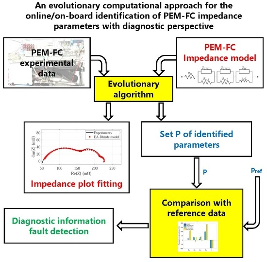
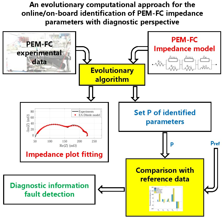
In this context, the main aim of this paper is to show that the PEM FC model-based identification of impedance parameters from an EIS-derived impedance spectrum can be performed online and on-board, with a diagnostic perspective. To this aim, an Evolutionary Algorithm (EA) is used due to its intrinsic ability to explore the search space and find the global optimum among multiple local ones.

EAs have already been used in various PEM FC optimization and identification problems, but very rarely in EIS identification or in online/on-board contexts. The identification problems are often based on the model reported in Reference [17], or similar ones. Their goal is to fit the FC voltage-to-current (V-I) polarization curve for diagnostic purposes (e.g., Reference [18] or Reference [19]). In Reference [20], an heuristic algorithm named Jaya is used for the optimization of a PEM FC stack design. The Jaya features are exploited to optimize the series/parallel connection of FCs and the cell active areas. This guarantees that the assembly delivers the rated voltage at the rated power, minimizing the overall system cost. In Reference [21], a stochastic optimization and a multiphysics performance model for the V-I curve are used for parametric identification. In Reference [22], a dynamic model is preferred and an offline identification is performed using Matlab™ environment. In Reference [23], an improved particle swarm optimization is utilized for the identification of a very detailed polarization curve model, again in offline mode. A less complex technique, such as a simple genetic algorithm, is used in Reference [24] for the estimation of parameters of a novel FC model.

The offline EIS data-driven identification of PEM FC equivalent circuits is also discussed in the literature. For instance, in References [25,26], least square-based algorithms or Matlab built-in tools are used. Some attempts were also made to extract diagnostic information from EIS time-domain data with a recursive filtering approach [27,28,29]. Few examples of online/on-board identification approaches oriented to FC diagnosis appeared in the literature. In Reference [30], a mix of evolutionary and deterministic algorithms is used to estimate the fractional order transfer function coefficients from time-domain sample data. This transfer function, which approximates the Warburg impedance, does not allow to obtain a good fit of the frequency-domain curve in healthy and faulty operating conditions. Consequently, poor information oriented to on-board diagnostics can be extracted from such frequency-domain parameters. The aforementioned Reference [30] does not provide neither a wide validation of the method in various FC operating conditions, nor an implementation of the algorithm on an embedded system. An alternative approach to online/on-board FC diagnostics is presented in Reference [11]. In that paper, a dimensionless aggregate indicator describes the overall condition of the FC stack. A dc-dc converter injects a PRBS stack current excitation, whose response is analyzed by using an algorithm based on the wavelet transform. This approach prevents the straightforward detection of the failure modes. Moreover, the PRBS sequence requires faster measurements than a sequence of tones at various frequencies but it requires a more significant computational effort.

This paper proposes a computational approach to the identification of the impedance parameters of a PEM FC stack model, based on an EA characterized by limited computational effort. The EA benefits from the use of sub-populations and migration among sub-populations. These features improve the exploration capability of the search space. The impedance parameter identification is formulated as an optimization problem. The objective function is defined as the mismatch between two impedance plots in a normalized plane. The first plot represents the experimental impedance and the second is computed on the basis of the identified parameters using a circuit model. Three kinds of impedance models, characterized by increasing computational complexity, are used depending on the experimental data to be fitted. The first one, a linear model made of resistors and capacitors, is particularly suitable for a low computational burden implementation. The second one is the so-called Fouquet model [14], that is frequently used in PEM FC literature for its accuracy in frequency-domain representation. The third one, called Dhirde model, extends the Fouquet model capabilities to more complicated impedance plots, characterized by peculiar low frequency behaviors. Preliminary analysis of the experimental impedance spectrum allows one to correlate groups of parameters in each model, or to reduce the initial search space of the algorithm in a valuable way, with beneficial effects on the computational burden. The algorithm is implemented on a low-cost off-the-shelf device, suitable to manage data acquisition in EIS experiments [3,31], with a C-language implementation. For the sake of comparison, Matlab implementation results are also shown. The method is validated with literature data in a simulated environment, as well as with experimental data. A good accuracy and low computation times are achieved with commercial embedded system hardware resources, proving that the computational approach fits well with the online/on-board requirements. Finally, from a diagnostic perspective, various experimental impedance plots for a PEM FC stack in normal and faulty conditions are shown. The effects of air and fuel starvation, and of water management issues [32], are analyzed. Then, a PEM FC diagnostic procedure is outlined on the basis of the identification outcomes.

The paper is organized as follows. Section 2 briefly recalls three FC stack models used throughout the paper, Section 3 describes the proposed computation approach to the EA, that is validated in Section 4 in simulation as well as with experimental results. Then, Section 5 discusses the diagnostic perspectives of the proposed computational approach. Finally, some conclusions are drawn in Section 6.

2. Fuel Cell Stack Models

In the neighborhood of a dc operating point, the FC stack can be modeled by various frequency-domain equivalent electric circuits representing the stack impedance. These models are characterized by various capability of reproducing the frequency-domain response of a FC and by various computational complexity, depending on the type of circuit elements included in the circuit.

The simplest circuit model is a linear resistive-capacitive (RC) impedance, that is, an impedance made of a series connection of a linear resistor with a number of RC parallel branches. This number is at least equal to one. The Nyquist-plane impedance plot corresponding to this circuit is characterized by the superposition of some circumference arcs, joined together.

More detailed models, suitable for complex-domain fitting, may include the so-called Warburg impedance and some CPEs in the parallel branches. These complex elements, having no corresponding lumped circuit element in the time-domain, enable one to draw impedance plots characterized by depressed and rectified arcs, typical of electrochemical systems [9].

Three models for the impedance are described in the following subsections—the RC model, Fouquet model, and Dhirde model. All of them share a linear resistor, $R_{\mathsf{\Omega }}$, accounting for the losses due to the resistance of the electrolyte to the flow of protons and appearing in series with the rest of the impedance. From a graphical point of view, the presence of this element shifts the impedance plot towards right, for a length equal to $R_{\mathsf{\Omega }}$. The shape of the plot is determined by the remaining elements appearing in the parallel branches.

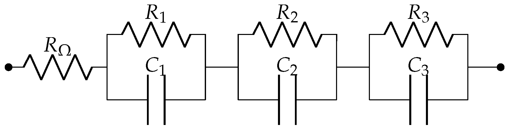
2.1. RC Model

This linear RC model includes the resistor $R_{\mathsf{\Omega }}$ and a number $N_{\mathrm{RC}}$ of RC parallel branches representing the main system dynamics. The equivalent circuit includes $N_p=2N_{\mathrm{RC}}+1$ parameters to be identified on the basis of the experimental impedance measurements at various frequencies. For instance, Figure 1 shows the third-order linear RC model ($N_{\mathrm{RC}}=3$).

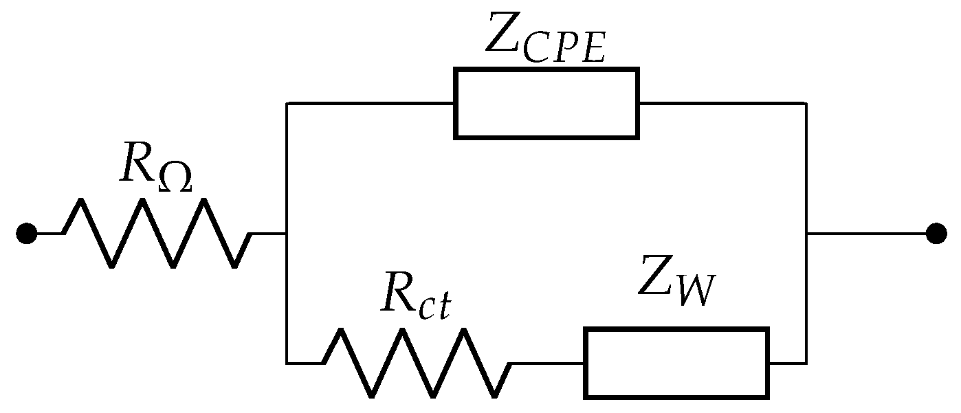
2.2. Fouquet Model

The Fouquet model includes both a CPE:

$$\begin{array}{cc}\hfill {\dot{Z}}_{\mathrm{CPE}}& =\frac{1}{Q{\left(j\omega \right)}^{\varphi }},\hfill \end{array}$$

(1)

and a Warburg element:

$$\begin{array}{cc}\hfill {\dot{Z}}_{\mathrm{W}}& =R_{\mathrm{d}}\frac{tanh\sqrt{j\omega {\tau }_{\mathrm{d}}}}{\sqrt{j\omega {\tau }_{\mathrm{d}}}},\hfill \end{array}$$

(2)

and neglects anodic phenomena. In (1) and (2), Q and $\varphi$ define the CPE, which represents the behavior of electrodes in the case of rough and porous surfaces. In the Warburg impedance, $R_{\mathrm{d}}$ accounts for the losses due to the diffusion of reactants, characterized by the time constant ${\tau }_{\mathrm{d}}$ [14]. The Fouquet impedance is depicted in Figure 2. Its expression is the following:

$$\dot{Z}=R_{\mathsf{\Omega }}+\frac{{\dot{Z}}_{\mathrm{CPE}}(R_{\mathrm{ct}}+{\dot{Z}}_{\mathrm{W}})}{{\dot{Z}}_{\mathrm{CPE}}+R_{\mathrm{ct}}+{\dot{Z}}_{\mathrm{W}}}.$$

(3)

Here, $\omega =2\pi f$ is the angular frequency, and $R_{\mathrm{ct}}$ is the charge transfer resistance, representing the resistance at the interface electrode/electrolyte to the flow of charges. The Fouquet model is characterized by six parameters ($N_p=6$).

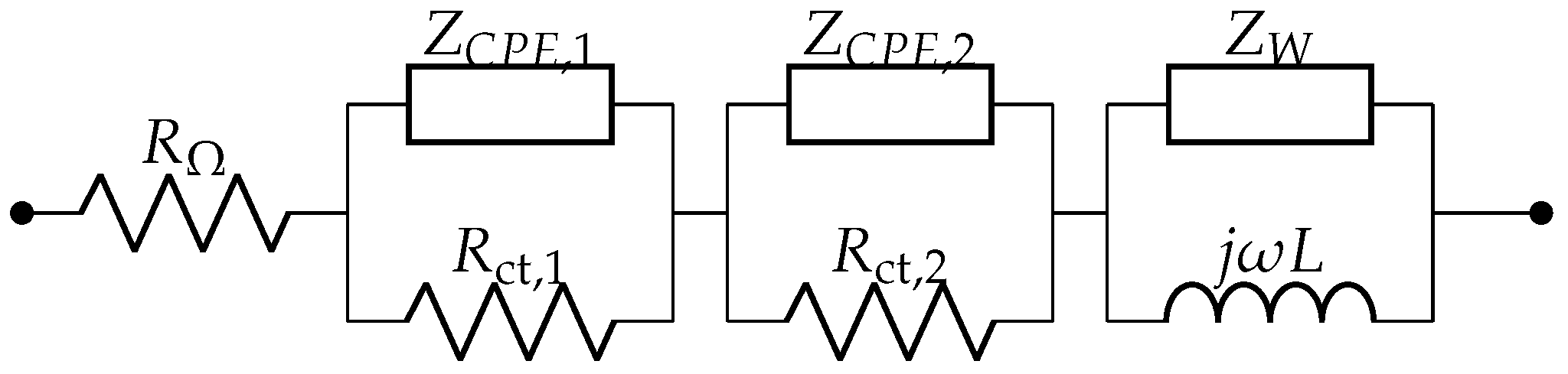
2.3. Dhirde Model

The Dhirde model also includes an inductive element, representing peculiar effects at low frequency. It could be particularly useful to fit a small depressed arc in the low-frequency range of the impedance plot. It was presented for the first time in Reference [15]. Figure 3 shows the Dhirde impedance, characterized by the presence of a Warburg element connected in parallel with the low frequency inductance and two CPEs. The overall impedance is:

$$\dot{Z}=R_{\mathsf{\Omega }}+\sum _{k=1}^2\frac{{\dot{Z}}_{\mathrm{CPE},k}{R}_{\mathrm{ct},k}}{{\dot{Z}}_{\mathrm{CPE},k}+R_{\mathrm{ct},k}}+\frac{j\omega L{\dot{Z}}_{\mathrm{W}}}{j\omega L+{\dot{Z}}_{\mathrm{W}}},$$

(4)

where ${\dot{Z}}_{\mathrm{W}}$ is defined in (2), and ${\dot{Z}}_{\mathrm{CPE},k}$ is defined, according to (1), as:

$$\begin{array}{cc}\hfill {\dot{Z}}_{\mathrm{CPE},k}& =\frac{1}{Q_k{\left(j\omega \right)}^{{\varphi }_k}}\mathrm{for}k=1,2.\hfill \end{array}$$

(5)

Here, L represents the low-frequency inductive behavior. The Dhirde model includes $N_p=10$ parameters.

3. The Evolutionary Algorithm

3.1. The Algorithm

An EA is an heuristic optimization algorithm based on the evolution of a population of possible solutions to the problem. The population evolves according to rules inspired by biology. The EA used in this paper is constructed on the scheme shown in Reference [33], by assuming that experimental measurements of the stack impedance:

$${\dot{Z}}_{\exp }\left(f_k\right)=R_{\exp ,k}+j{X}_{\exp ,k},$$

(6)

are available for all frequency points $f_k$, $k=1,\dots ,M$.

The individual evolving generation by generation is a vector of $N_p$ genes, that is, real numbers representing the circuit parameters. Each gene is coded as a 64-bit floating point real number, whose values are bounded according to the physical meaning of each parameter. If the linear RC model is used, all the genes, either representing a resistance or a capacitance, are merely forced to be strictly positive. If the Fouquet model is considered, parameters $R_{\mathsf{\Omega }},R_{\mathrm{ct}},Q,R_d,{\tau }_d$ are forced to be positive, while $\varphi$ lies in $\left[-1,1\right]$, according to Reference [14]. Similar constraints are imposed in the case of Dhirde impedance, with the addition of a constraint on L, which is forced to be strictly positive. The width of these physical ranges, which in some cases is very large, leads to a slow EA convergence. This issue will be discussed in Section 3.5.

3.2. The Objective Function

Once the stack model is selected, for each individual in the EA population, the impedance:

$${\dot{Z}}_{\mathrm{num}}\left(f_k\right)=R_{\mathrm{num},k}+j{X}_{\mathrm{num},k}$$

(7)

is evaluated at each frequency value $f_k$, $k=1,\dots ,M$. In these points, ${\dot{Z}}_{\exp }\left(f_k\right)$ is also available. Introducing the following constants:

$$\begin{array}{cc}\hfill R_{\max }& =max{\left\{|R_{\exp ,k}|\right\}}_{k\in \{1,\dots ,M\}},\hfill \end{array}$$

(8)

$$\begin{array}{cc}\hfill X_{\max }& =max{\left\{|X_{\exp ,k}|\right\}}_{k\in \{1,\dots ,M\}},\hfill \end{array}$$

(9)

the normalized real and imaginary parts of the impedance are defined by:

$$\begin{array}{cccc}\hfill & r_{\exp ,k}=\frac{R_{\exp ,k}}{R_{\max }},\hfill & \hfill & r_{\mathrm{num},k}=\frac{R_{\mathrm{num},k}}{R_{\max }}\hfill \end{array}$$

(10)

$$\begin{array}{cccc}\hfill & x_{\exp ,k}=\frac{X_{\exp ,k}}{X_{\max }},\hfill & \hfill & x_{\mathrm{num},k}=\frac{X_{\mathrm{num},k}}{X_{\max }}.\hfill \end{array}$$

(11)

These normalized quantities are included in the definition of the normalized objective function ${\mathcal{F}}_{\mathrm{obj}}$, or fitness function:

$${\mathcal{F}}_{\mathrm{obj}}=\frac{1}{M}\sum _{k=1}^M\sqrt{{\left[r_{\mathrm{num},k}-r_{\exp ,k}\right]}^2+{\left[x_{\mathrm{num},k}-x_{\exp ,k}\right]}^2},$$

(12)

whose value has to be minimized by the EA. Here, ${\mathcal{F}}_{\mathrm{obj}}$ is computed by averaging the distance between experimental and numerical impedance points in a normalized real-to-imaginary plane. This definition takes into account the shape of the impedance spectrum, as well as the proximity between experimental and numerical impedance at the same frequency $f_k$. The latter aspect is often neglected in many model-based parameter identification approaches appearing in the literature, for instance in Reference [34].

3.3. The Sub-Populations

A classical EA implementation uses only one set of individuals, namely a population. Each population represents a possible solution to the optimization problem [33]. Here, sub-populations are introduced according to a migration model, in order to preserve useful genetic diversity among individuals across generations, and in order to avoid trapping the algorithm in local optima [35,36,37]. The migration model divides the population in multiple sub-populations, also known as demes. These sub-populations evolve independently from each other for a certain number of generations, called isolation time or epoch. After each isolation time, a number of individuals is distributed among the sub-populations, thus the migration takes place. The number of exchanged individuals (migration rate), the method for selection of migrating individuals, and the scheme of migration determine the amount of genetic diversity in the sub-populations and the amount of information exchanged among sub-populations.

In the algorithm used in this paper, the individuals are selected for the migration on the basis of their objective function value (12). A ring topology migration scheme [38] is adopted: after each epoch, which is one complete computation for all individuals, the $N_{\mathrm{best}}$ best individuals from the j-th sub-population migrate to the $(j+1)$-th sub-population, by replacing the worst individuals, and from the last population towards the first one.

The introduction of migration in the algorithm has two beneficial effects: first, an improvement in the EA success rate [37] and, second, an improvement in the time performance [39]. Indeed, with the same total number of individuals, migration allows a faster convergence of the algorithm, as it encourages the exploration of various areas of the search space [37,39]. Usually, migration enables the use of smaller populations than that one evolving in a single run, with the same performance. Here, the migration model has been preferred to other parallel evolutionary methods, such as the global model, or the diffusion model. It is worth noticing that the migration model is suitable for a parallel implementation, with a possible reduction of the computation time. Moreover, such an approach requires less objective function computations than those required by a single population algorithm. As a consequence, the parallel algorithm, even if applied to a single processor (pseudo-parallel), finds the global optimum more often, or at least with fewer function evaluations [37]. From a computational point of view, the implemented algorithm behaves as a kind of parallel EA, which takes benefit from running on a multi-core processors. Nowadays, such processors are also available on low-cost embedded systems, Field-Programmable Gate Arrays (FPGAs), or in an actual System-On-Chip (SOC).

3.4. Selection, Crossover and Mutation Operators

In order to reduce the computational complexity of the algorithm, the tournament selection method is employed [33]. The tournament method is particularly suitable for implementation in embedded systems with low computational resources. A number of tournaments, equal to the number of individuals to be selected for reproduction, is performed by randomly taking a set of individuals from the population, and by selecting the one having the lowest objective function value among them. Rank scaling selection is also implemented by means of the stochastic universal sampling. According to this method, a simple technique allocates reproduction opportunities to individuals. The tournament selection approach gives weaker members of a population a chance to be chosen according to their fitness function value, and thus it reduces the unfair nature of fitness-proportional selection methods, requiring a greater computational effort.

The single-point crossover operator is adopted [33]. Two parent chromosomes are split into two parts in a randomly-selected point. The left sub-chromosome of one parent, and the right sub-chromosome of the other parent are collected, giving rise to the first child, while the remaining sub-chromosomes, joined together, constitute the second child. Using a neat cut within genes, the real crossover operator is equivalent to the binary one—each child will lie in the intersection of two hyper-planes determined by its parents.

The adaptive feasible mutation strategy is used. The operator mutates the gene according to a normal distribution, whose mean value is equal to the gene actual value. The standard deviation of such a distribution reduces progressively while the EA goes towards the converge. The mutation keeps into account the range in which the search is performed. Indeed, if the lower or upper limit of the range is reached, the mutation changes its versus, that is, the mutation sign.

3.5. Search Space and Parameter Correlations

According to the parameter bounds described in Section 3.1, the search space is extremely wide, with a negative effect on the convergence rate of the algorithm. Even the optimal set of parameters might lead to an impedance ${\dot{Z}}_{\mathrm{num},k}$ far from ${\dot{Z}}_{\exp ,k}$. In order to address this problem, the physical meaning of the experimental data is taken into account. Indeed, the EIS is usually performed in a frequency range such that the impedance plot crosses the real axis in two points. The two intercepts $R_{\exp }^{\left(\mathrm{HF}\right)}$ and $R_{\exp }^{\left(\mathrm{LF}\right)}$, with $R_{\exp }^{\left(\mathrm{HF}\right)}<R_{\exp }^{\left(\mathrm{LF}\right)}$, that is, the two impedance values whose imaginary parts vanish, can either be determined or extrapolated from experimental data. These experimental values can be used in the algorithm in two different ways. The first approach is to relate them directly to some resistances appearing in the model, reducing the order of the problem. Alternatively, the aforementioned intercepts of the impedance spectrum with the real axis can help to reduce the search space size along one specific parameter.

According to the first approach, in all models reported in Section 2, $R_{\exp }^{\left(\mathrm{HF}\right)}$ is equal to the ohmic resistance $R_{\mathsf{\Omega }}$, so that this value is initially set and the number of unknown parameters reduces to $N_p-1$.

For the linear model, the low-frequency intercept, $R_{\exp }^{\left(\mathrm{LF}\right)}$, is the sum of all the resistances appearing in the model, so that:

$$R_3=R_{\exp }^{\left(\mathrm{LF}\right)}-R_{\exp }^{\left(\mathrm{HF}\right)}-R_1-R_2.$$

(13)

Therefore, the knowledge of both intercepts defines a constraint among the model resistances, and scales the problem down to five unknowns, that is, according to (13): $R_1,R_2,C_1,C_2,C_3$.

Similar conclusion is drawn for the remaining models. For Fouquet model (see Figure 2), (13) is replaced by:

$$\begin{array}{cc}\hfill & R_{\mathrm{ct}}=R_{\exp }^{\left(\mathrm{LF}\right)}-R_{\exp }^{\left(\mathrm{HF}\right)}-R_d.\hfill \end{array}$$

(14)

In this case, the individual is characterized by the following reduced set of four parameters: $\left[Q,\varphi ,R_d,{\tau }_d\right]$.

In a similar way, for Dhirde model (see Figure 3), (13) is replaced by:

$$\begin{array}{cc}\hfill & R_{\mathrm{ct},1}+R_{\mathrm{ct},2}=R_{\exp }^{\left(\mathrm{LF}\right)}-R_{\exp }^{\left(\mathrm{HF}\right)},\hfill \end{array}$$

(15)

which enables the computation of $R_{\mathrm{ct},2}$ as a function of $R_{\mathrm{ct},1}$.

In the presence of missing intercepts or noisy data, it could be worth not applying this constraint to the algorithm. As an alternative approach, the search space of some specific resistances can be reduced in a valuable way. To this aim, a neighborhood of the experimental values can be used instead of wide intervals. This approach filters out the noise affecting the experimental data, and avoids constraining the identification, with a beneficial effect on the overall residue. This latter approach is preferred in all the cases presented hereafter. This choice may lead to a small deviation of parameters with respect to their own mean (for instance, this will happen to $R_{\mathsf{\Omega }}$) but it helps finding the optimal solution.

4. Experimental Results

Two sets of experimental results are used to validate the method. The first set comes from the characterizations of a six-cell assembly with an active area of 150 cm², whose results are presented in Reference [14]. The second set comes from experiments performed in the frame of the H2020 HEALTH-CODE project [3], characterized by various faults, such as those described in Reference [40].

The EA runs with a population of $N=200$ individuals, 4 sub-populations with 50 individuals each, whose $10\%$ is allowed to migrate from one sub-population to another one. The tournament selection and a single point crossover operators are used, with a crossover probability $P_{\mathrm{C}}=60\%$. The epoch is fixed at $E=333$. The initial mutation probability is $P_{\mathrm{M}}=20\%$. This value is halved when the population heterogeneity reduces. At each step, given the objective function value ${\mathcal{F}}_{\mathrm{obj}}^{*}$ computed for the best individual of the population, the halving is performed as soon as the mean value $\overline{{\mathcal{F}}_{\mathrm{obj}}}$ of ${\mathcal{F}}_{\mathrm{obj}}$, computed over the population, falls below the fixed threshold ${ϵ}_1=20\%$:

$$\begin{array}{c}\hfill \overline{{\mathcal{F}}_{\mathrm{obj}}}<{ϵ}_1{\mathcal{F}}_{\mathrm{obj}}^{*}.\end{array}$$

(16)

The EA converges when at least one of the following conditions occurs: (i) the number of generations is equal to $N_{\mathrm{gen}}=$ 10,000; (ii) ${\mathcal{F}}_{\mathrm{obj}}$ improvement for 50 successive generations is below ${ϵ}_2={10}^{-6}$; (iii) the value of the objective function falls below a fixed threshold ${ϵ}_3={10}^{-3}$.

The algorithm is coded both in Matlab and in C language. The latter implementation is aimed at running on an embedded system. Matlab code runs on a PC with Intel Core i7-4720HQ at $2.60 \mathrm{GHz}$. The C-language code runs on a Beagle Bone Black (BBB) REV C. The BBB supports a single core AM335x $1 \mathrm{GHz}$ ARM Cortex-A8 processor, and it is equipped with 512 MB DDR3 RAM, 4 GB 8-bit eMMC on-board flash storage, a NEON floating-point accelerator and a 2x PRU 32-bit microcontrollers. Debian 7.9 OS runs on the board. In the tables showing the results, BBB times are reported. Matlab computation times are also included as reference values.

4.1. Validation by Literature Data with RC and Fouquet Model

In this test, the FC behavior is simulated to obtain the set of experimental impedance points ${\dot{Z}}_{\exp ,k}$ for all k. To this aim, the Fouquet model is run in M frequency points by using the following data: $R_{\mathsf{\Omega }}=4.5 \mathrm{m}\mathsf{\Omega }$, $R_{\mathrm{ct}}=8.1 \mathrm{m}\mathsf{\Omega }$, $Q=1.8056$, $\varphi =0.8419$, $R_{\mathrm{d}}=3.6 \mathrm{m}\mathsf{\Omega }$, ${\tau }_{\mathrm{d}}=0.1919 \mathrm{s}$. These data are taken from Reference [34].

Once the reference experimental impedance ${\dot{Z}}_{\exp ,k}$ has been obtained for all k, the EA is run to identify the parameters of the three models described in Section 2. The most interesting results are obtained by using the RC model and the Fouquet model. The results reported in

Table 1. Identification on Fouquet data [14] by using the third order linear model.

Parameter	Best	Mean	$\mathit{\sigma }$
$R_{\mathsf{\Omega }}$ (m$\mathsf{\Omega }$)	4.514	4.515	3.17·10${}^{-3}$
$R_1$ (m$\mathsf{\Omega }$)	4.230	2.457	1.331
$R_2$ (m$\mathsf{\Omega }$)	5.296	4.987	1.233
$R_3$ (m$\mathsf{\Omega }$)	2.132	4.209	1.343
$C_1$ (F)	20.69	20.95	0.1829
$C_2$ (F)	1.7286	2.202	0.3345
$C_3$ (F)	0.8865	0.8830	2.430·10${}^{-3}$
Matlab time (s)	3.87	15.87	12.07
BBB time (ms)	0.258	0.765	0.438
${\mathcal{F}}_{\mathrm{obj}}$ (m$\mathsf{\Omega }$)	9.075	9.861	1.250

(for RC model) and in

Table 2. Identification on Fouquet data [14] by using the Fouquet model.

Parameter	Best	Mean	$\mathit{\sigma }$
$R_{\mathsf{\Omega }}$ (m$\mathsf{\Omega }$)	4.498	4.496	0.0490
$R_{\mathrm{ct}}$ (m$\mathsf{\Omega }$)	8.199	8.038	0.786
Q	1.866	1.875	0.09742
$\varphi$	0.8366	0.8334	0.05016
$R_{\mathrm{d}}$ (m$\mathsf{\Omega }$)	3.501	3.669	0.8150
${\tau }_{\mathrm{d}}$ (s)	0.1938	0.2089	0.01734
Matlab time (s)	2.18	10.39	4.88
BBB time (ms)	0.861	2.46	1.68
${\mathcal{F}}_{\mathrm{obj}}$ (m$\mathsf{\Omega }$)	0.954	6.487	6.756

(for Fouquet model) are graphically shown in Figure 4. For each parameter, the best individual, the mean one and its standard deviation $\sigma$ are listed. The mean individual and the standard deviation are computed over 100 independent EA runs. These runs are launched by starting from a randomly-generated initial population. Considering the results of the Fouquet model in the best case (see Table 2), they are very close to the ones used to generate the reference plot. The computation time required by the C-language implementation is reported in the second part of the Tables. The Matlab time is also given for comparison purposes. It is worth highlighting that Matlab implementation benefits from many built-in functions.

Figure 4 shows the impedance plots corresponding to the best individuals. The identification results achieved by both models satisfactorily fit the reference plot. The presence of two arcs is correctly detected. The Fouquet model is characterized by higher fitting fidelity, whose measure is the ${\mathcal{F}}_{\mathrm{obj}}$ value. Indeed, in the best Fouquet case, ${\mathcal{F}}_{\mathrm{obj}}$ is lower than the one obtained by means of the RC model. The success rate of the EA is 96% for Fouquet model. This leads to an apparent spread of the solutions over a wide interval, as suggested by the $\sigma$ value affecting ${\mathcal{F}}_{\mathrm{obj}}$ in Table 2, as well as some parameters. Indeed, in this case, the mean value and the standard deviation are very close to one another. This happens both to the objective function and to some parameters. Excluding the 4 unsuccessful cases over 100, in which the EA shows a premature convergence to a local optimum, the mean value of ${\mathcal{F}}_{\mathrm{obj}}$ becomes very close to the best one, with a standard deviation that drops below $10 \mathsf{\mu }\mathsf{\Omega }$. The standard deviation of the parameters changes accordingly.

Looking at the computation time required by the BBB device to run the EA, the average time required to run the RC model is 70% less than the time required to run the Fouquet model. Indeed, the Fouquet model shows a higher computational burden with respect to the RC model because of its non-linearity, and this aspect has a significant impact especially on the embedded system implementation. Conversely, the RC circuit represents a good compromise between the fitting accuracy of the impedance spectrum and the computation time.

4.2. Validation by Experimental Dataset A with RC and Fouquet Model

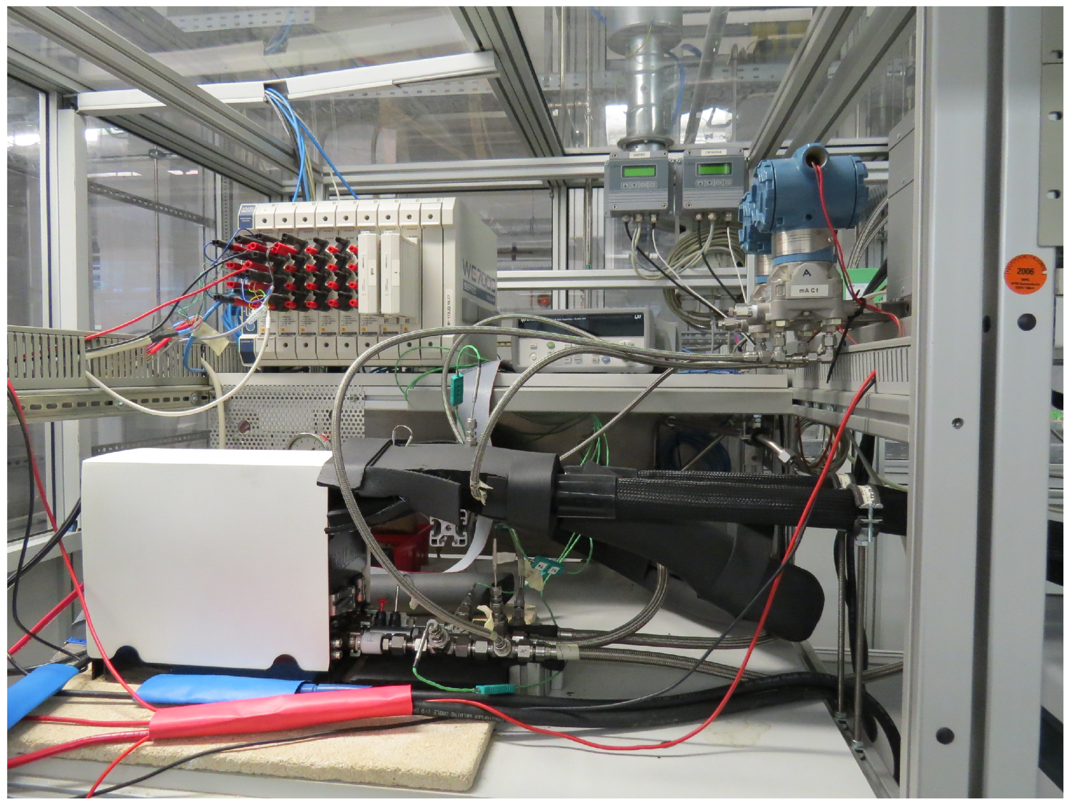
Further analyses are performed by using experimental data. The dataset A collects the data obtained in the framework of the H2020 HEALTH-CODE project [3], by testing a 46-cell PEM FC stack from Ballard Power System (see Figure 5). The stack was tested at $0.4 \mathrm{A}/{\mathrm{cm}}^2$, and $57 °\mathrm{C}$, under nominal and faulty conditions: cathode and anode drying, hydrogen starvation, and oxygen starvation are considered. The nominal operating conditions were defined by inlet gases’ relative humidity of 83%, and respective anodic and cathodic overstoichiometric ratios of 1.3 and 2. In all the experiments, the fuel was a mixture of 76% H${}_2$, 20% CO${}_2$ and 4% N${}_2$, a composition similar to a reformate gas produced on-board by an alternative carbon-based fuel, such as methanol. The use of reformate gas seems to be more practical than considering pure hydrogen.

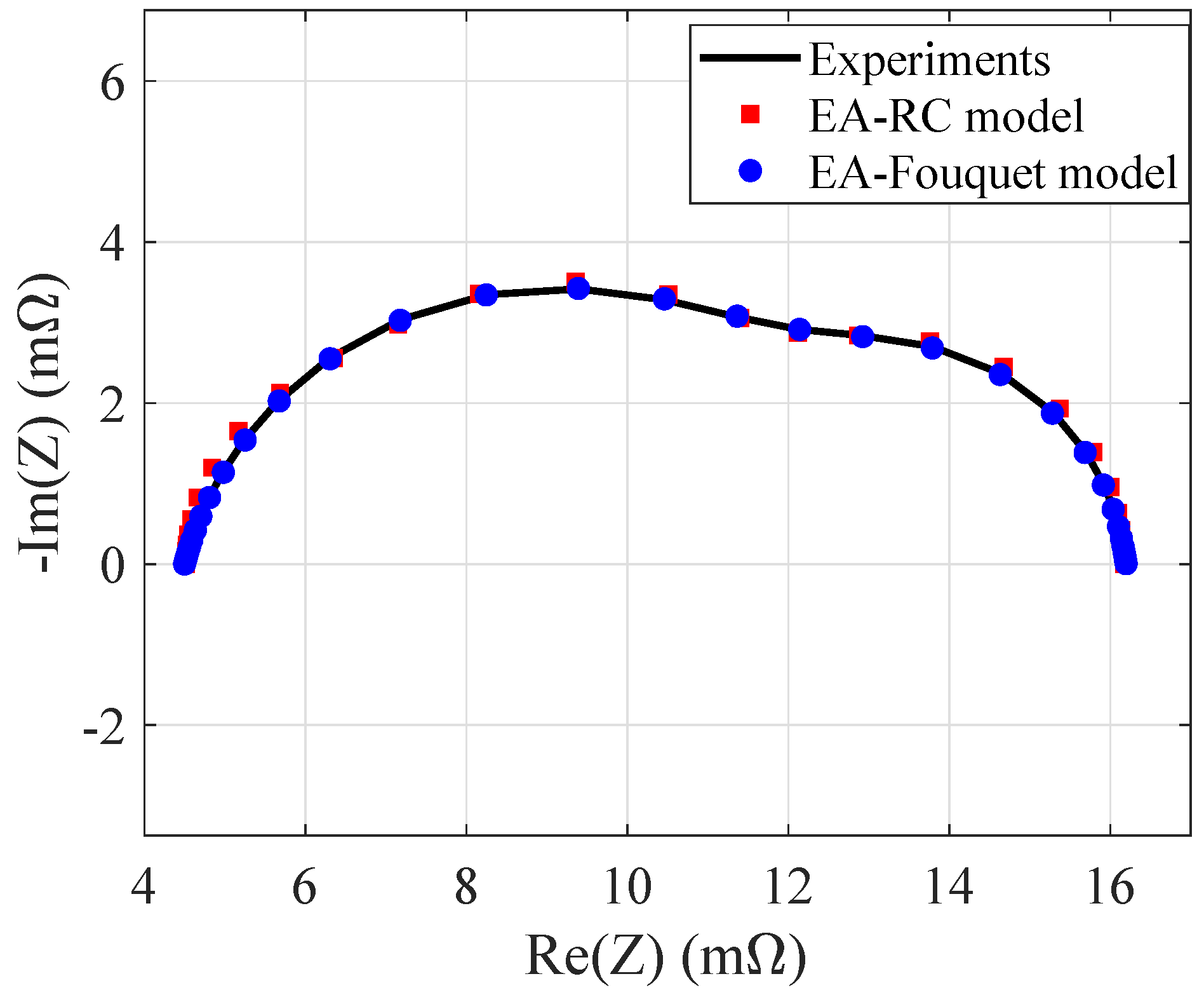
Figure 6 shows the good identification performed by both models, with a computation time required by the BBB within $2 \mathrm{ms}$, on average. The two-arcs shape of the impedance plot is quite accurately detected by both models.

Table 3. Dataset A. EA identification results (linear model).

Parameter	Best	Mean	$\mathit{\sigma }$
$R_{\mathsf{\Omega }}$ (m$\mathsf{\Omega }$)	55.63	55.61	0.0584
$R_1$ (m$\mathsf{\Omega }$)	36.95	36.81	0.9730
$R_2$ (m$\mathsf{\Omega }$)	52.51	52.61	0.8150
$R_3$ (m$\mathsf{\Omega }$)	50.48	50.50	0.1580
$C_1$ (F)	0.0340	0.0340	0.0001
$C_2$ (F)	0.1483	0.1476	0.0056
$C_3$ (F)	1.934	1.9293	0.0115
Matlab time (s)	9.880	27.48	9.500
BBB time (ms)	0.4700	0.9830	0.5460
${\mathcal{F}}_{\mathrm{obj}}$ (m$\mathsf{\Omega }$)	0.0294	0.0294	2.7$·{10}^{-5}$

and

Table 4. Dataset A. EA identification results (Fouquet model).

Parameter	Best	Mean	$\mathit{\sigma }$
$R_{\mathsf{\Omega }}$ (m$\mathsf{\Omega }$)	51.51	51.02	1.070
$R_{\mathrm{ct}}$ (m$\mathsf{\Omega }$)	101.3	103.6	4.815
Q	0.1689	0.1807	0.0256
$\varphi$	0.7369	0.7258	0.0232
$R_{\mathrm{d}}$ (m$\mathsf{\Omega }$)	44.78	43.08	3.378
${\tau }_{\mathrm{d}}$ (s)	0.2203	0.2222	0.0043
Matlab time (s)	8.230	43.25	15.06
BBB time (ms)	1.218	1.7680	0.3390
${\mathcal{F}}_{\mathrm{obj}}$ (m$\mathsf{\Omega }$)	0.0392	0.0437	0.0031

report on the results. Again, the computation time required by the RC model is lower than the one obtained with Fouquet model, confirming that C-language implementation suffers from the presence of complex-valued elements, such as the CPEs.

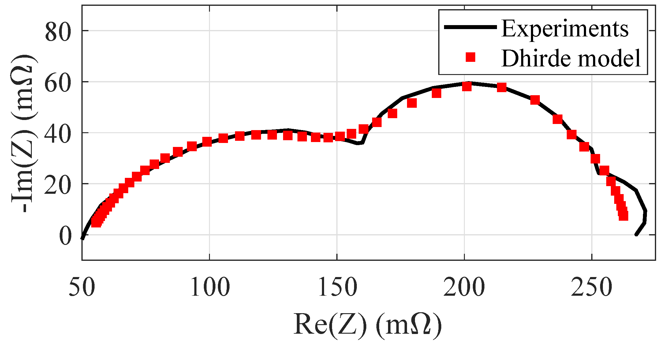
4.3. Validation by Experimental Dataset B with Dhirde Model

The dataset B is a further set of experimental results used for the validation. The data were acquired by the same test-bed described in Section 4.2. The low-frequency behavior is characterized by a peculiar shape, which does not allow to achieve low values of ${\mathcal{F}}_{\mathrm{obj}}$ when RC model or Fouquet model are used. To address this problem, the identification of this dataset is carried out by using the Dhirde model, implemented in Matlab. Dhirde model is characterized by $N_p=10$ parameters. In this case, the EA runs with a population larger than the ones used before: $N=1000$ individuals.

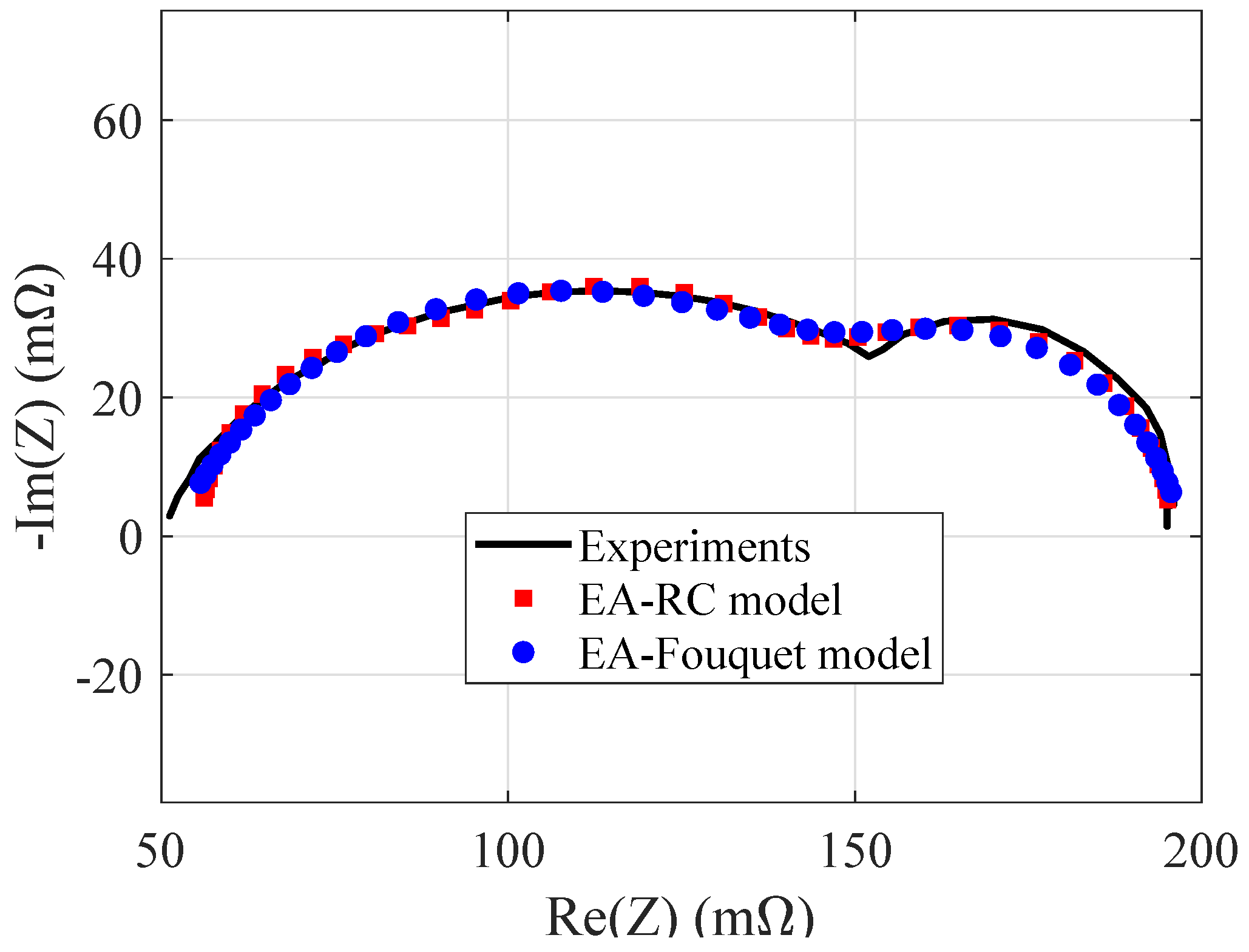
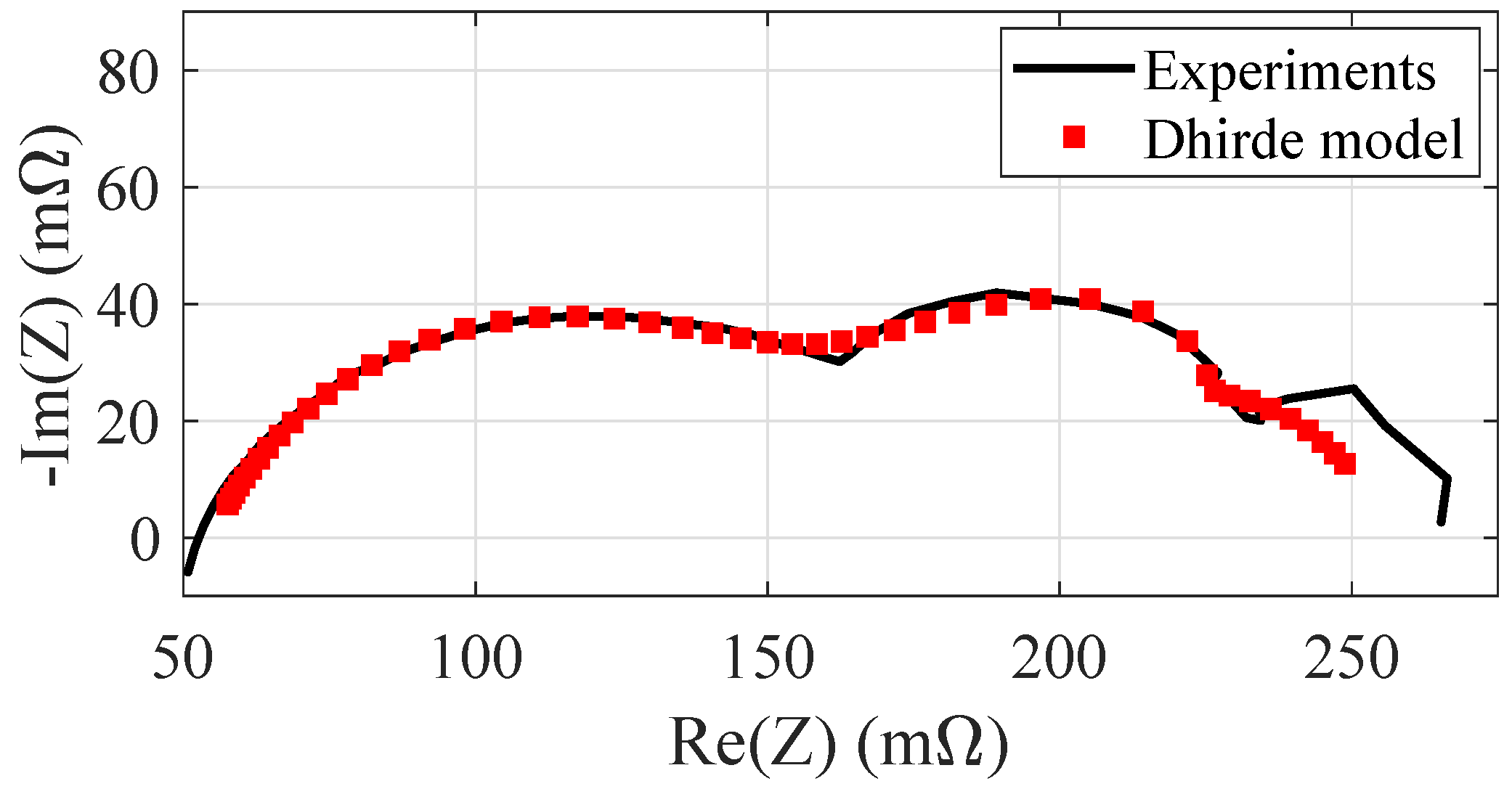
Compared to previous analyses, considering the valuable increase of both the population and the number of parameters, identification times are expected to be substantially higher. Figure 7 shows the identification results achieved by the Dhirde model when the FC stack works in nominal conditions at $40 \mathrm{A}$. The right hand side of the plot clearly shows the good fit achieved by the Dhirde model in the presence of a third arc located in the low frequency range.

Table 5. Experimental dataset B. Identification results in normal operative conditions with Dhirde model.

Parameter	Value	Parameter	Value
$R_{\mathsf{\Omega }}$ (m$\mathsf{\Omega }$)	54.20	$Q_1$	2.953
$R_{\mathrm{ct},1}$ (m$\mathsf{\Omega }$)	46.30	$Q_2$	0.1731
$R_{\mathrm{ct},2}$ (m$\mathsf{\Omega }$)	113.4	${\varphi }_1$	1.000
$R_{\mathrm{d}}$ (m$\mathsf{\Omega }$)	15.90	${\varphi }_2$	0.705
${\tau }_{\mathrm{d}}$ (s)	7.8886	L (mH)	47.10
Matlab time (s)	93.28	${\mathcal{F}}_{\mathrm{obj}}$ (m$\mathsf{\Omega }$)	26.7

summarizes the identification results over 100 independent EA runs, as already done in previous tables. The computation time required by the EA with Dhirde model is obviously higher than the Fouquet or RC ones. As a future perspective, in order to tackle this point and reduce the computation time, the intrinsic parallel evolution of the sub-populations can be exploited and a part of the EA can be parallelized.

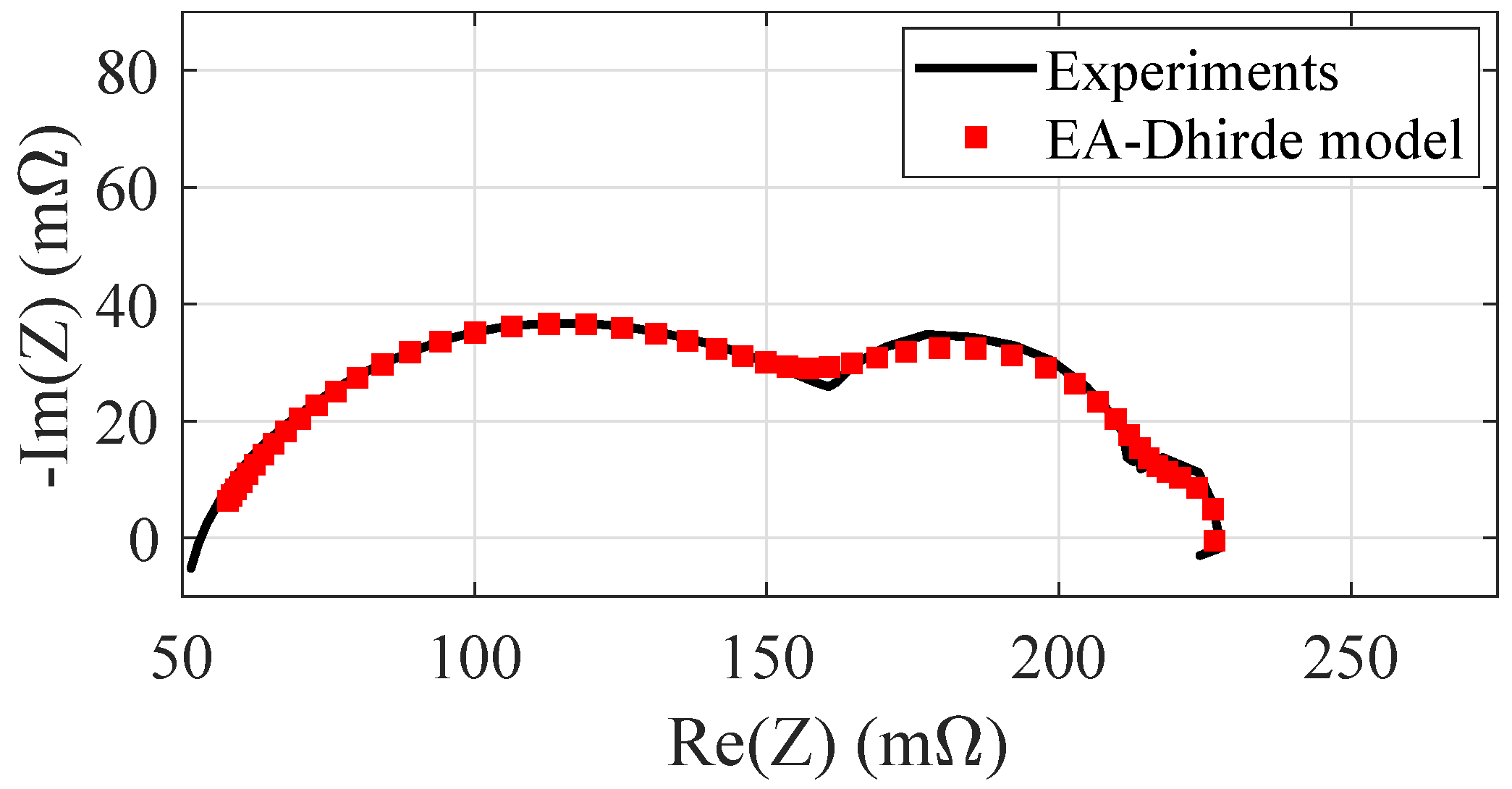
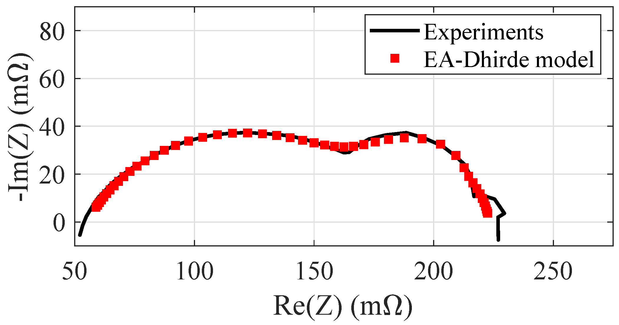
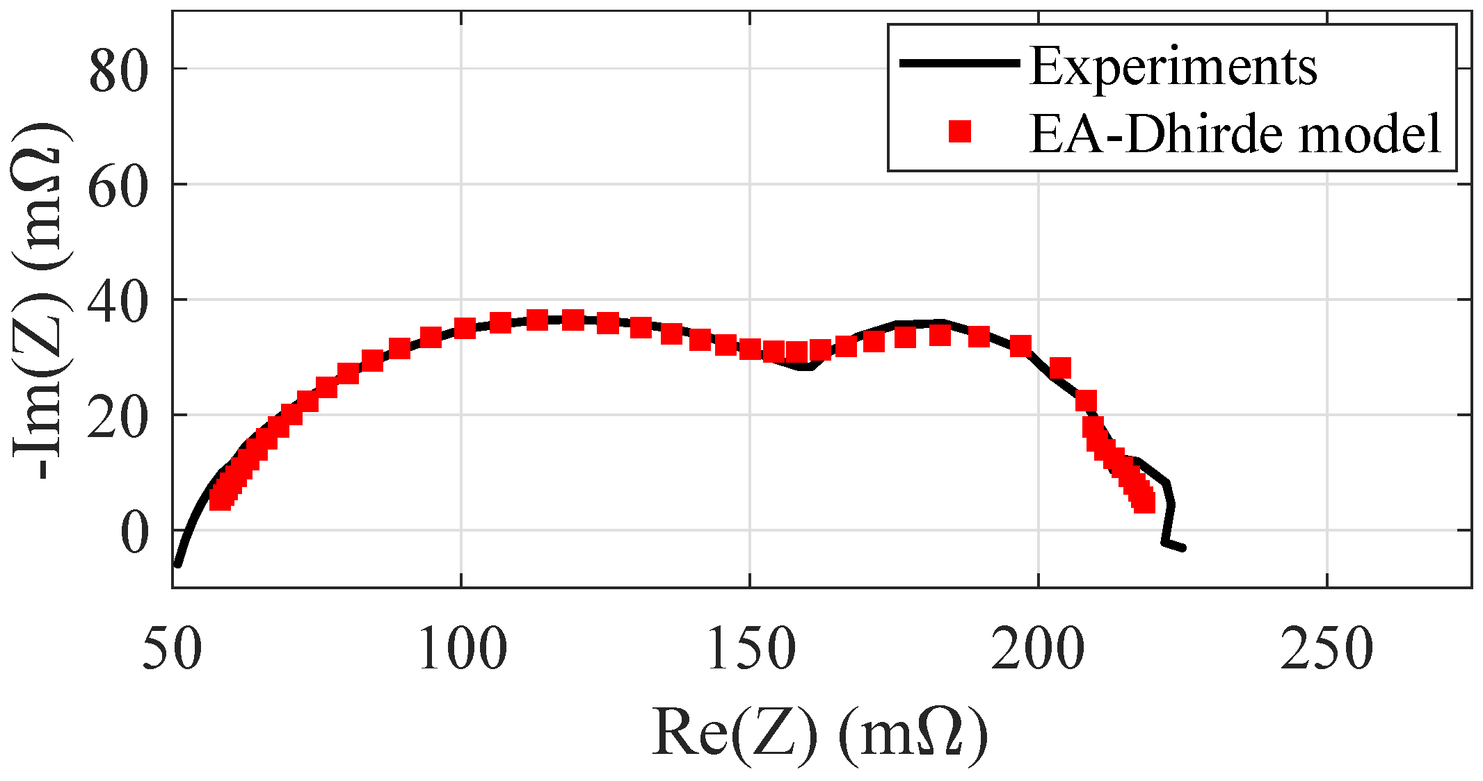
5. Identification Oriented to Diagnostics

In order to capture how the variations of Dhirde model parameters can be correlated to faults, more spectra are identified both in normal and faulty operating conditions. This is done in a diagnostic perspective. As already mentioned in Section 4.3, the Dhirde model appears the most suitable one for this kind of identification problem, having already shown good identification capabilities in the presence of the low-frequency third arc. 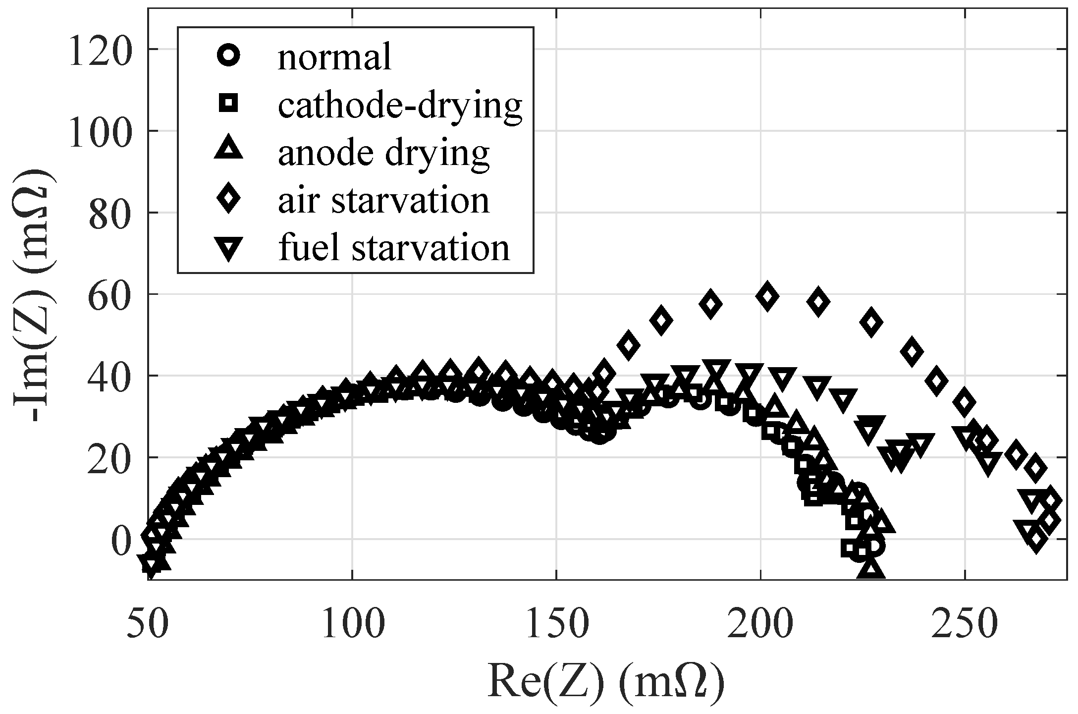Here, the following faults are considered—cathode and anode drying (see Figure 8 and Figure 9), air and fuel starvation (see Figure 10 and Figure 11). In these figures, each identified spectrum is compared to the experimental one. The analysis is carried out again through Matlab only. In order to compare the various behaviors in normal and faulty conditions, the whole set of experimental data is shown in a comprehensive way in Figure 12. Using the Dhirde model, the parameters are identified by the EA in all faulty cases, ending up with the values reported in

Table 6. Comparison among the parameters identified in various operating conditions at 40A nominal current. The number of arrows highlights, in a qualitative way, the percentage variation x with respect to nominal condition. $\uparrow :10\%\le x<50\%$, $\uparrow \uparrow :50\%\le x<100\%$, $\uparrow \uparrow \uparrow :x\ge 100\%$. ↓, $\downarrow \downarrow$, and $\downarrow \downarrow \downarrow$ are defined accordingly.

Parameter	Normal Condition	Cathode Drying		Anode Drying		Air Starvation		Fuel Starvation
$R_{\mathsf{\Omega }}$ ($\mathsf{\Omega }$)	0.0542	0.0554		0.0549		0.0528		0.0546
$R_{\mathrm{ct},1}$ ($\mathsf{\Omega }$)	0.0463	0.0584	↑	0.0477		0.0966	$\uparrow \uparrow \uparrow$	0.0997	$\uparrow \uparrow \uparrow$
$R_{\mathrm{ct},2}$ ($\mathsf{\Omega }$)	0.1134	0.1063		0.1209		0.1142		0.1027
$Q_1$	2.9533	3.9406	↑	3.8822	↑	2.4108	↓	3.9387	↑
$Q_2$	0.1731	0.1959	↑	0.2368	↑	0.2472	↑	0.1598	$\downarrow \downarrow$
${\varphi }_1$	1.0000	0.8725	↓	0.9999		1.0000		0.7469
${\varphi }_2$	0.7050	0.7150		0.6719		0.7010		0.7321
$R_{\mathrm{d}}$ ($\mathsf{\Omega }$)	0.0159	0.0316	$\uparrow \uparrow$	0.0319	$\uparrow \uparrow \uparrow$	0.0453	$\uparrow \uparrow \uparrow$	0.0456	$\uparrow \uparrow \uparrow$
${\tau }_{\mathrm{d}}$ (s)	7.8861	5.9740	↓	8.9543	↑	6.0082	↓	6.5949	↓
L (H)	0.0471	0.0023	$\downarrow \downarrow$	0.0015	$\downarrow \downarrow$	0.0028	$\downarrow \downarrow$	0.0037	$\downarrow \downarrow$

. The arrows highlight the main parameter variations with respect to the normal condition. The number of arrows is related to the magnitude of variation for each parameter, as detailed in the caption of Table 6.

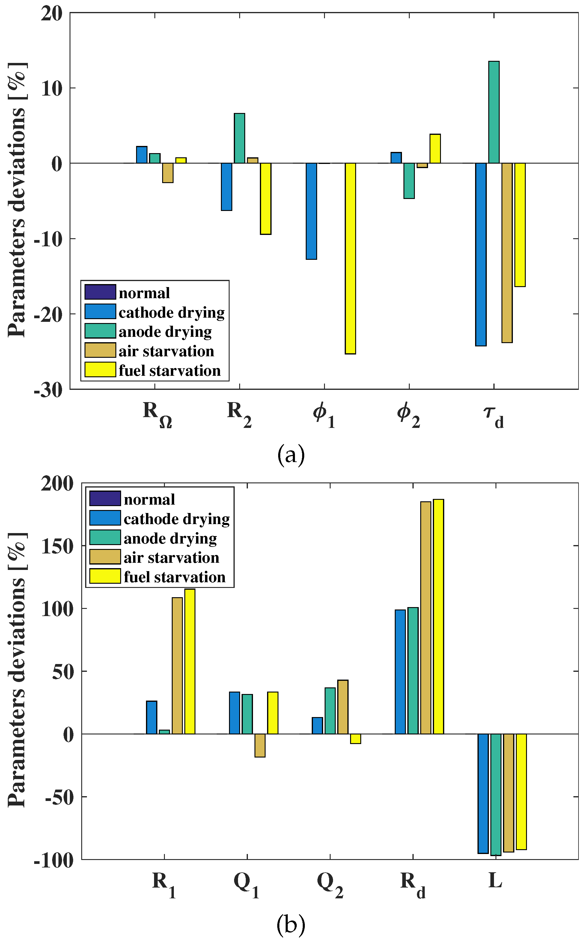
Figure 13 shows the same variation in a pictorial and more intuitive way. Figure 13a shows the parameters exhibiting low variations, while Figure 13b shows those ones characterized by high variation. Each bar represents the percent variation of each parameter appearing in the Dhirde model with respect to normal operating conditions. The different colors refer to the analyzed fault conditions. These figures reveal that, according to the Dhirde model, all the faults considered are characterized by a significant reduction of L and an increase of $R_d$. Briefly:

• Fault Condition (FC) = $(\Delta L<0)$ & $(\Delta R_d>0)$.

If this happens, and if an increase of $Q_1$ occurs, then a drying fault is detected:

• Drying Condition (DC) = (FC) & $(\Delta Q_1>0)$.

Alternatively, in the presence of a strong increase of $R_{\mathrm{ct},1}$, a starvation fault is detected:

• Starvation Condition (SC) = (FC) & $(\Delta R_{\mathrm{ct},1}>0)$.

Moreover, in drying fault conditions, the strong increase or decrease of ${\tau }_{\mathrm{d}}$ allows one to distinguish between cathode and anode drying, respectively:

• Cathode Drying (CDC) = (DC) & $(\Delta {\tau }_{\mathrm{d}}<0)$,
• Anode Drying (ADC) = (DC) & $(\Delta {\tau }_{\mathrm{d}}>0)$.

Finally, in starvation conditions, the parameter $Q_2$ indicates whether air or fuel starvation is occurring. Briefly:

• Air Starvation (ASC) = (SC) & $(\Delta Q_2>0)$,
• Fuel Starvation (FSC) = (SC) & $(\Delta Q_2<0)$.

All the variations highlighted in Table 6 or Figure 13 could be used to define fault conditions. Such a method points out the diagnostic potential of the EA computational approach. At present, the diagnostic method is sketched on the basis of very few experiments. Further work is needed to extensively test the identification capability of the EA algorithm, which deeply affects the reliability of the diagnostic procedure. This should be done on the basis of a wider experimental dataset, in which more experimental data are available for each single fault. On the basis of a comprehensive statistics, which is beyond the scope of this paper, the aforementioned methodology should be refined and integrated.

6. Conclusions

In this paper, an evolutionary computation approach to the identification of the impedance parameters of polymeric electrolyte membrane fuel cells is proposed for online/on-board electrochemical impedance spectroscopy experiments. The identification of the impedance parameter is formulated as an optimization problem and solved with an evolutionary algorithm. The knowledge of high- and low-frequency intercepts of the impedance plot with real axis allows one to define some constraints among parameters or to reduce the algorithm search space. The use of sub-populations and migration among sub-populations attain good exploration of the search space and represent a promising solution.

Many tests validate the computational approach by using both simulated and experimental data. Accurate experimental data fitting, with an error lower than $1\%$, is achieved, especially by using the Fouquet model for fuel cell impedance. A few milliseconds, or even less, are required to identify the set of parameters when the algorithm runs on a low-cost off-the-shelf embedded system. The lowest computation times are achieved by using a linear resistive-capacitive model. The identification time is very short, making this computational approach to the evolutionary algorithm suitable for online and on-board applications.

From the perspective of a fuel cell stack diagnosis based on estimated impedance parameter, both normal and faulty condition data are identified. This is done to study whether the faults can be detected on the basis of parameter variations with respect to normal conditions.

Further work is in progress in order to implement the evolutionary algorithm in an embedded system with hardware parallel computation capabilities, such as a field programmable gate array. This will enable a parallel objective function computation for many individuals or, additionally, a parallel evolution of the sub-population. In this way, a further reduction of the identification time is expected. Concerning the fault detection procedure outlined in this paper, a further effort is aimed at improving it on the basis of more experimental data, in order to increase its robustness and reliability.

References