Optimal Dispatch of Aggregated HVAC Units for Demand Response: An Industry 4.0 Approach

Abstract

Demand response (DR) involves economic incentives aimed at balancing energy demand during critical demand periods. In doing so DR offers the potential to assist with grid balancing, integrate renewable energy generation and improve energy network security. Buildings account for roughly 40% of global energy consumption. Therefore, the potential for DR using building stock offers a largely untapped resource. Heating, ventilation and air conditioning (HVAC) systems provide one of the largest possible sources for DR in buildings. However, coordinating the real-time aggregated response of multiple HVAC units across large numbers of buildings and stakeholders poses a challenging problem. Leveraging upon the concepts of Industry 4.0, this paper presents a large-scale decentralized discrete optimization framework to address this problem. Specifically, the paper first focuses upon the real-time dispatch problem for individual HVAC units in the presence of a tertiary DR program. The dispatch problem is formulated as a non-linear constrained predictive control problem, and an efficient dynamic programming (DP) algorithm with fixed memory and computation time overheads is developed for its efficient solution in real-time on individual HVAC units. Subsequently, in order to coordinate dispatch among multiple HVAC units in parallel by a DR aggregator, a flexible and efficient allocation/reallocation DP algorithm is developed to extract the cost-optimal solution and generate dispatch instructions for individual units. Accurate baselining at individual unit and aggregated levels for post-settlement is considered as an integrated component of the presented algorithms. A number of calibrated simulation studies and practical experimental tests are described to verify and illustrate the performance of the proposed schemes. The results illustrate that the distributed optimization algorithm enables a scalable, flexible solution helping to deliver the provision of aggregated tertiary DR for HVAC systems for both aggregators and individual customers. The paper concludes with a discussion of future work.

1. Introduction

1.1. Context and Motivation

With improved connectivity, dramatically increased access to low-cost computational power and recent advances in data science, many industries are currently on the verge of a second digital revolution known as ‘Industry 4.0’ [1]. Of the many challenges which can be addressed by Industry 4.0, concepts of sustainable, highly available plants and fully integrated renewable energy are prominent [1,2]. This involves aspects of industrial digitalization related to real-time, distributed and robust system-wide optimization methods coupled with the tighter integration of control, scheduling, planning and demand-side management for industrial production systems and energy networks [1,2]. The focus of this paper lies in the use of HVAC and/or refrigeration systems within buildings to provide aggregated energy-shifting services for demand response (DR) purposes within an Industry 4.0 framework. Building stock is estimated to account for around 40% of global energy consumption, exceeding that of other major sectors like industry and transportation [3,4]. As such, buildings represent the sector with both the largest energy saving and energy shifting potential for DR applications [3,4].

DR is the generic title given to a range of options customers have to reduce costs and/or generate profits by changing their pattern of consumption; economic benefits can be leveraged by deliberately moving consumption away from peak/critical times, or deliberately moving consumption onto off-peak/critical times [4,5,6]. Figure 1 illustrates the concept of DR. Heating, ventilation and air conditioning (HVAC) of buildings provides the largest possible source for this energy saving and energy shifting potential [4,5]. The opportunities for realizing demand response vary across Europe, as they are dependent on the particular regulatory, market and technical contexts in different European countries [4]. Nevertheless, successful DR programs are becoming increasingly common for large industrial customers. However, DR programs aimed at small and medium scale customers have mostly failed to meet their expected potential. Previous research has identified that blocks (or groups) of buildings offer more flexibility for the provision of DR than single buildings, the latter of which are generally too limited in capacity to operate individually in power markets [4,5,6,7,8,9]. As such, researchers and the energy industry are beginning to consider how blocks of buildings can operate collectively within energy networks to enhance the effectiveness of DR programs. The potential value of DR in blocks of buildings depends on the telemetry and control technologies embedded in the building management systems currently deployed at any given site and the potential revenue sources: both of which can vary significantly according to specific local and national conditions [4]. In this context, to encourage the growth of DR services and reap the potential benefits of DR, it is necessary for current research to demonstrate the economic and environmental benefits of DR for the different key actors required to bring DR services in blocks of buildings to market.

There are several established and emerging DR archetypes suitable for use with individual buildings and blocks or groups of buildings, e.g., see [4,6,7]. This paper is principally concerned with explicit (surgical) DR, in which prior notification is given to the DR participant of a pending event and its requirements for down-regulation or up-regulation of demand during a specified future time window. In the UK market, for example, the DR archetypes of short-term operating reserve (STOR) and demand turn up (DTU) are employed [6]. For both STOR and DTU events, enrolled participants are notified of an upcoming event and its requirements typically between 30–240 min before the required time of delivery (although day-ahead notice is sometimes given), and event durations are of at least 120 min [6]. STOR and DTU event windows occur at differing periods during the day (peak and off-peak, respectively) and require an aggregated minimum of three MW to be available. This latter restriction is also a motivating factor for considering blocks of buildings. In general, STOR and DTU can be considered as tertiary forms of reserve DR (ancillary services), which can be integrated alongside emerging fast-acting and very fast-acting decentralized approaches for providing secondary and primary frequency regulation services using HVAC systems, e.g., see [7,9].

1.2. Related Work

There is a growing body of work studying direct load control (DLC) techniques for HVAC units and other thermostatically controlled loads (TCLs) such as refrigerators. The fundamental requirements of DLC are outlined in an earlier work, which presents a general optimization framework for feeder-scale load reduction [10]. A priority-based control scheme for TCLs to participate in grid frequency regulation has also been developed [11]. A two-stage dispatch method has been demonstrated for TCLs in which a day-ahead scheduling model is solved to determine the optimal TCL dispatch, and then a real time control model allocates the desired setpoints to individual TCLs [12]. The use of a Markov transition matrix to model the populated TCLs to carry out non-disruptive load reduction underpins other work [13]. Previous work also makes use of thermal inertia models to control TCL in smart homes [14], and research has been conducted to propose a model for coordinated dispatch of TCLs and thermal generation units [15].

Motivated by the observation that users are not immediately convinced that replacing existing thermostats by an intelligent controller is worth the investment, a ‘reference governor’ approach for optimizing performance and energy consumption of building thermostatically controlled loads was developed in an earlier work [16]. In this research, a model predictive control (MPC) supervisory unit adjusts the temperature setpoints for a relay controlling the on/off load. The MPC problem is converted into a mixed-integer linear programing (MILP) problem, which is dispatched in real-time. Although the method is shown to be effective, it is restricted to a single heating/cooling zone, and little consideration is given in the earlier research to implementation details such as communication or computation overheads.

In all the above research and technical developments, the on/off control actions of individual TCLs are driven by the thermostat settings and DR actions are principally achieved by varying setpoints within pre-set temperature ranges. However, other work has sought to aggregate TCLs in numerous buildings. For example, Luo et al. [8] presented a framework for aggregating TCLs in a rolling-horizon framework, aimed principally at the Nordic electricity market. Standard thermal comfort models described by International Organization for Standardization (ISO) standard ISO 7730 are adopted to estimate occupant thermal comfort in a representative model for TCL dispatch. To avoid the technical intractability of dispatching TCLs individually in a large-scale centralized model, similar TCLs are first grouped based on feature similarities using a clustering technique and an averaged TCL model for each group is then created. A randomized meta-heuristic technique named the natural aggregation algorithm (NAA) is then employed to dispatch the averaged TCLs in each combined group. Since both the number of groups and the number of NAA iterations can be pre-selected, the computation time can be tailored to suit available resources; however, this is at the expense of solution sub-optimality. Although the technique is shown to give good results on practical examples, the optimal solution cannot be guaranteed [8].

Callaway [17] also describes a statistical model for aggregating TCLs such that frequency regulation services can be provided in the presence of generation variability. This work presents a new DR method to provide load following services by controlling the aggregated TCLs under Fokker–Planck diffusion models [17]. A minimum-variance (MV) statistical control law is derived to follow a one-step-ahead load signal and is demonstrated to perform well under simulation with 10,000 TCLs. Zhou et al. [18] developed a change-time-priority-list method to control power output taking into account customers’ satisfaction for the aggregation of multiple HVAC systems to provide demand-side frequency regulation services, to support intermittency of renewable generation, e.g., in the presence of fluctuating wind power. The aggregation unit employs simple approximations for on/off change times in the HVAC units to prioritize their dispatch in order to follow load control signals. Simulations verify the tracking ability of the system when connected to 6000 TCLs.

In the earlier works discussed above, the proposed methods are shown to perform favorably, but large numbers of aggregated units (>1000) are needed for the statistical approximations to be accurate; this limits their down-scalability and they cannot be applied to situation of, say, ten HVAC units. In addition, the lack of a rigorous baselining scheme for participant settlement—and potentially high communication load between an aggregator (providing the means by which individual HVAC unit owners can participate in DR) and individual units—are major drawbacks from a practical perspective.

1.3. Contributions

In this paper, an efficient and partially decentralized approach to aggregated tertiary DR schemes for individual or blocks of buildings is proposed. As with other Internet-of-Things and Industry 4.0 applications, large-scale DR implementation across multiple HVAC units across different geographic locations results in large volumes of high-velocity real-time data, and very large optimization and scheduling problems that must be solved centrally. It is beneficial to run local processing of these data at the edge of the network (on ‘edge devices’) to reduce the frequency and real-time requirements of communication to core devices in such situations [2]. In addition, in an Industry 4.0 context, it makes sense to distribute the optimization and resource scheduling problems between the network edges and core as much as possible. This is the approach taken in the research presented here.

Initially, the paper focuses upon the dispatch problem for individual TCLs in the presence of a tertiary DR program. The dispatch problem for an individual HVAC zone is formulated as a non-linear constrained predictive control problem, which manipulates on/off controls to optimize thermal comfort and electricity consumption across a future time horizon. A dynamic programming (DP) algorithm is developed to solve the dispatch problem with fixed memory and computation time overheads, rendering it suitable to be implemented as an intelligent thermostat unit (ITU), which can be implemented on an edge device with IP communications. A key factor of the implementation is the exposure of adjustable constraints, which can be used to enforce a minimum and/or maximum level of control activity during a specified window of time. This allows electricity consumption to be increased (or decreased) during a specified DR window. In the absence of DR signals, the DP solution defaults to a simple thermostat with adjustable deadzone; this allows the ITU to calculate an accurate baseline in the presence of active DR signals to ensure consumption is surgically reduced (increased) to a specified level during a DR event, and post-settlement can be effectively handled.

The paper also presents an efficient unit allocation/reallocation scheme (UAS) for aggregated explicit DR employing multiple ITUs. The UAS is employed by an aggregator to allocate individual DR targets to individual zones based upon advertised price/energy relationships. It can also be employed to reallocate targets should an individual unit drop out from, or drop in to, an upcoming DR event, or should environmental conditions indicate that a previously allocated target for a unit cannot be achieved. The UAS is formulated as a modified knapsack algorithm, which can be efficiently solved using DP techniques, and is designed to be cloud-based and hosted in the network core. As such, the proposed ITU/UAS overall exhibits low bandwidth requirements—as only elementary data need to be periodically exchanged between the aggregator and ITUs. Additionally, the computational load is distributed evenly across the core and network edges and optimization workloads are executed in parallel for each of the ITUs.

A number of computational simulations and a large-scale experimental test are then described to verify and illustrate the performance of the proposed schemes. It is argued that the ITU optimization algorithm for individual HVAC zones, combined with the centralized UAS procedure, enables a scalable, flexible solution helping to deliver the provision of aggregated tertiary DR for HVAC systems in distributed environments for both aggregators and individual customers.

1.4. Structure

The remainder of this article is structured as follows. In Section 2 and Section 3, the main technical developments are described in detail, including the assumed HVAC thermal dynamic model and the ITU/UAS optimization schemes. In Section 4, calibrated simulation studies and experimental results from practical tests are presented to illustrate the performance of the proposed schemes. Section 5 provides conclusions and suggestions for future areas of work.

2. Models and Assumptions

In this paper, the focus is principally upon explicit (surgical) DR events involving HVAC units. For ease of exposition, for the remainder of this paper it is assumed that the DR events to be handled are characterized by STOR-type events, in which prior notification of an upcoming event is given and the goal during the event is to reduce demand by a pre-agreed or negotiated amount. Since STOR-type events and DTU-type events are mutually exclusive, it is a relatively straightforward matter to modify the basic approach to handle DTU-type DR events, in which prior notification is again given but the goal during the event is to increase demand by a pre-agreed or negotiated amount. Figure 2 shows the assumed temporal relations between the key events in a STOR DR situation.

A variety of different modelling approaches (of varying complexity) for HVAC and building thermal dynamics can be found in the literature (see, e.g., [19]). Most models are based on physical principles related to mass, energy and momentum transfer and consist of complex partial differential equations that capture the building thermal and physical characteristics. Although the optimization to be developed in Section 3 allows for the use of complicated non-linear models, in practice simplified first-order models can typically perform just as well as more complicated models [17,20]. The descriptions and technical development henceforth consider the linear case for ease of exposition. In addition, for simplicity the assumption is also made that the unit in question delivers heated or cooled water to the building radiators, but may be applied to other configurations (e.g., hot air delivery) with an appropriate change of variables and/or model. Assuming continuous time indexed by the variable t, the linear dynamic relationship between the HVAC control signal u(t) ∊ {0, 1}, which switches electrical power delivery to the electro-thermal converter, the circulating water temperature delivered to the building T(t) and the (ambient) inlet water temperature T_A(t) is assumed to be well approximated by a first-order differential equation, as follows:

$$\dot{T}(t)=\frac{1}{\tau }(T(t)-T_A(t)+u(t-D)\cdot K_T),$$

(1)

where the dot above a variable represents its first derivative (d/dt), D ≥ 0 represents any dead-time in the converter dynamics, τ is the thermal time constant of the converter and K_T is the equivalent thermal gain of the converter. A model such as this has previously been studied in the context of HVAC control for demand response applications, and time constants of 10–30 min and dead-times between 0–5 min are typical of most buildings [17,18,19,20]. In Equation (1), the sign of K_T distinguishes between a heating (positive) or cooling (negative) application. Neglecting the standby power consumption, the variable electrical power consumption of the HVAC unit E(t) is determined by the state of the control signal and the electrical gain of the converter K_E, such that E(t) = u(t) K_E. Hence, as is well known, the HVAC unit may participate in STOR and DTU DR programs by modulating the electrical power consumption through deliberate under- or over-supply of thermal power, at the possible expense of some thermal comfort of the building occupants. Digitizing the Equation (1) for a time-step of T_s seconds, using k as the (integer) discrete-time index, yields:

$$T(k)=a\cdot T(k-1)+(1-a)\cdot \left[u(k-d)\cdot K_T-T_A(k-1)\right],$$

(2)

where the real parameter a = exp(−T_s/τ) > 0 and the integer d = 1 + (D/T_s), which if fractional is assumed rounded to the nearest whole integer. For the thermal model, Equation (1), it is suggested that the time step be chosen to be not more than 5% of the time constant τ. The reasoning behind this is that basic systems theory gives the open loop rise time of the model, Equation (1), as 2.2τ, and hence choosing T_s as suggested gives at least 44 time steps in the rise time, which should be adequate for good on/off control without leading to excessively short time steps (which could be problematic from an implementation viewpoint). For example, a 30-min time constant gives step times of not more than 90 s. The digitized model, Equation (2), provides a means in which the temperature evolution may easily be predicted over a future time horizon, enabling predictive optimization to be applied at each time step. The proposed optimization approaches are described in the following section.

3. Technical Development

The main technical development consists of three main elements: firstly, the ITU dispatch algorithm for an individual HVAC unit (Section 3.1); secondly, the approach to generate predictions of baseline and reduced consumption for an individual HVAC unit (Section 3.2); and thirdly, the UAS optimization approach for aggregated units (Section 3.3).

3.1. Individual Unit Dispatch

The legacy mode of operation of an HVAC unit for temperature control is typically through thermostat type controls, i.e., setting the control signal u(k) according to the simple ‘relay with hysteresis’ control law [7,17,18]:

$$u(k)=\{\begin{array}{cc}1,& T(k)\le T_R(k)-\Delta ;\hfill \\ u(k-1),& T_R(k)-\Delta \le \Delta T(k)\le T_R(k)+\Delta ;\hfill \\ 0,& T(k)\ge T_R(k)+\Delta ;\hfill \end{array},$$

(3)

where T_R(k) represents the temperature setpoint at time step k, and the deadzone of the relay (during which the output is held at its last value) is given by 2Δ. Such a mode of operation is simple to implement; in the following, it is wished to extend the basic relay-based approach to situations in which pre-heating (cooling) can be optimally managed for explicit DR events. For this, a rolling-horizon non-linear MPC employing a finite discrete input set is developed [20]. The optimization problem to be solved at each discrete-time step k is the minimization of the following multi-stage quadratic cost function:

Minimize:

$$J(k)={\displaystyle \sum _{i=0}^M{(T(k+i+d)-T_R(k+i+d))}^2}+\lambda {\displaystyle \sum _{i=0}^{M-1}\Delta u{(k+i)}^2}$$

(4)

with respect to:

$$u(k+i),0\le i\le M-1;$$

(5)

subject to:

$$\begin{array}{c}T(k+i+d+1)=a\cdot T(k+i+d)+(1-a)\cdot (u(k+i)\cdot K_T+T_A(k+i+d)),\\ 0\le i\le M-1;\end{array}$$

(6)

$$u(k+i)\in \{0,1\},0\le i\le M-1;$$

(7)

$$U_L\le {\displaystyle \sum _{i=0}^{M-1}(u(k+i)\cdot w(k+i))}\le U_U,$$

(8)

where T(k) represents the zone temperature at time slot k, T_R(k) represents the zone temperature reference (setpoint) at time slot k and T_A(k) represents the ambient temperature at time slot k. The binary decision variable u(k) represent the control input at time slot k and Δ is the difference operator such that Δu(k) = u(k) − u(k − 1). The scalar term λ is used to penalize changes in the control input and can be considered a ‘move suppression’ or regularization term. Integer d ≥ 1 represents the time delay and w(k) ∊ {0, 1} are indicator variables for defining a demand response window, such that DR is active during time slot k if w(k) is ‘1’ and not active otherwise. 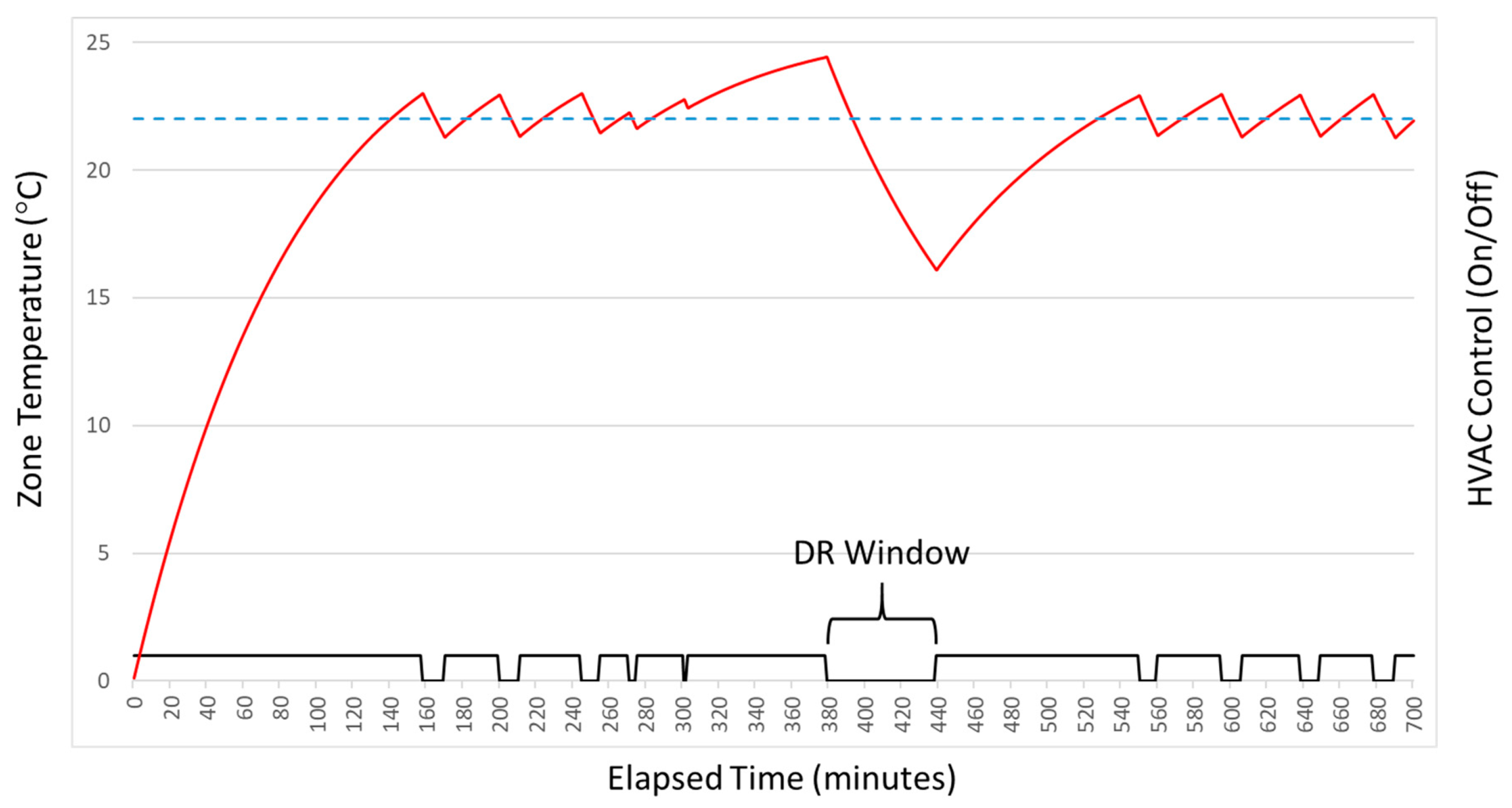The integer M represents the length of the prediction horizon, and integers U_U and U_L represent upper and lower bounds on the allowed input activity during a defined DR window. Henceforth in this paper, only an upper bound on control activity (e.g., for handling STOR-style DR events) is considered, with the understanding that adding the lower bound (e.g., for DTU-style DR events) follows directly from the described methods. 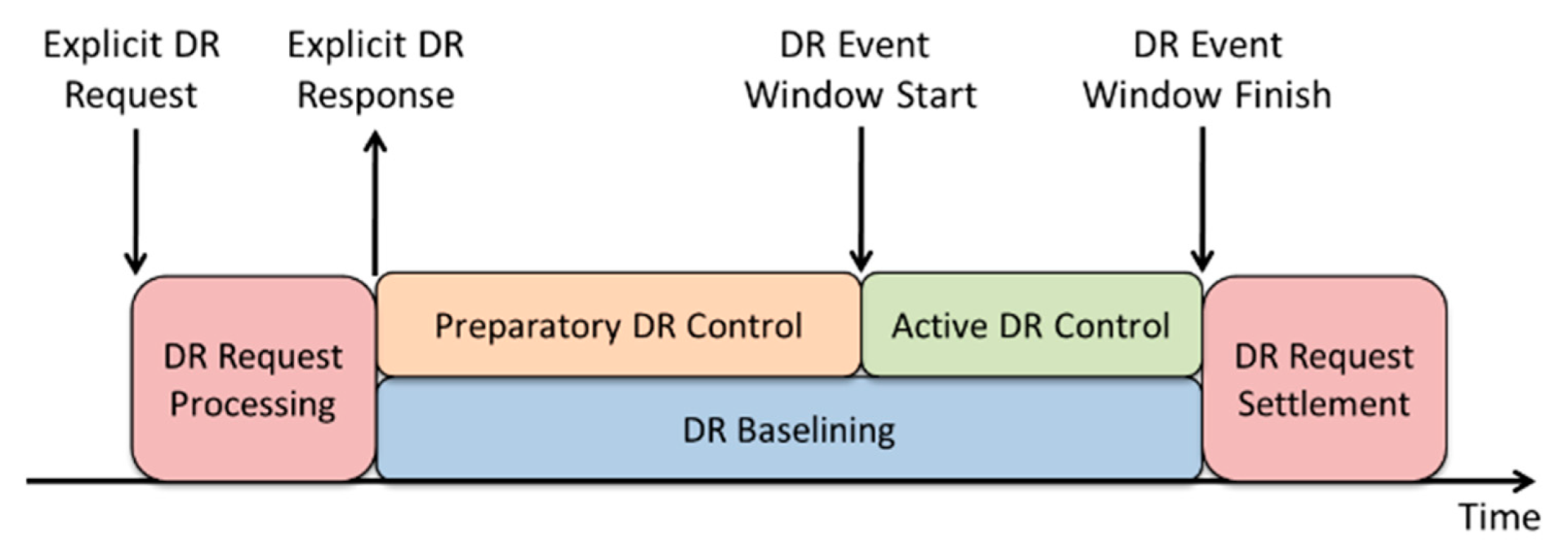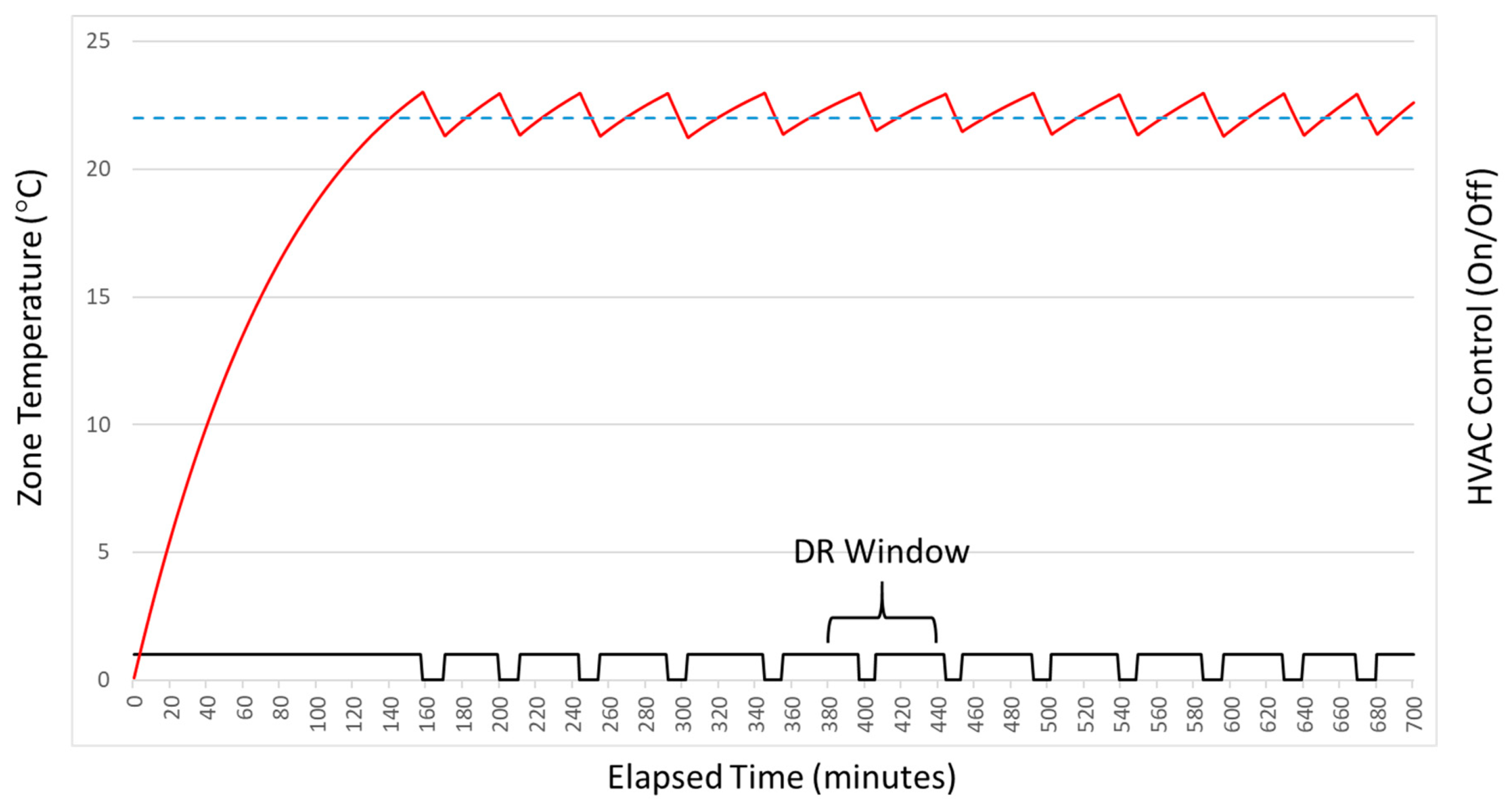As with other predictive control problems, an appropriate length for the prediction horizon would be the number of samples required to capture the open-loop setting time of the process [21]. However, with reference to Figure 2, this should be extended somewhat to allow for preparatory control actions to also take place. For the thermal model, Equation (1), basic systems theory gives the settling time as 4.6τ, giving a suggested horizon length M = ⌈(4.6τ + W)/T_s⌉, where W is the length of time required for preparatory control. For example, a 30-min time constant and preparatory window W of one hour with time step of 90 s gives a horizon length M of 132 steps.

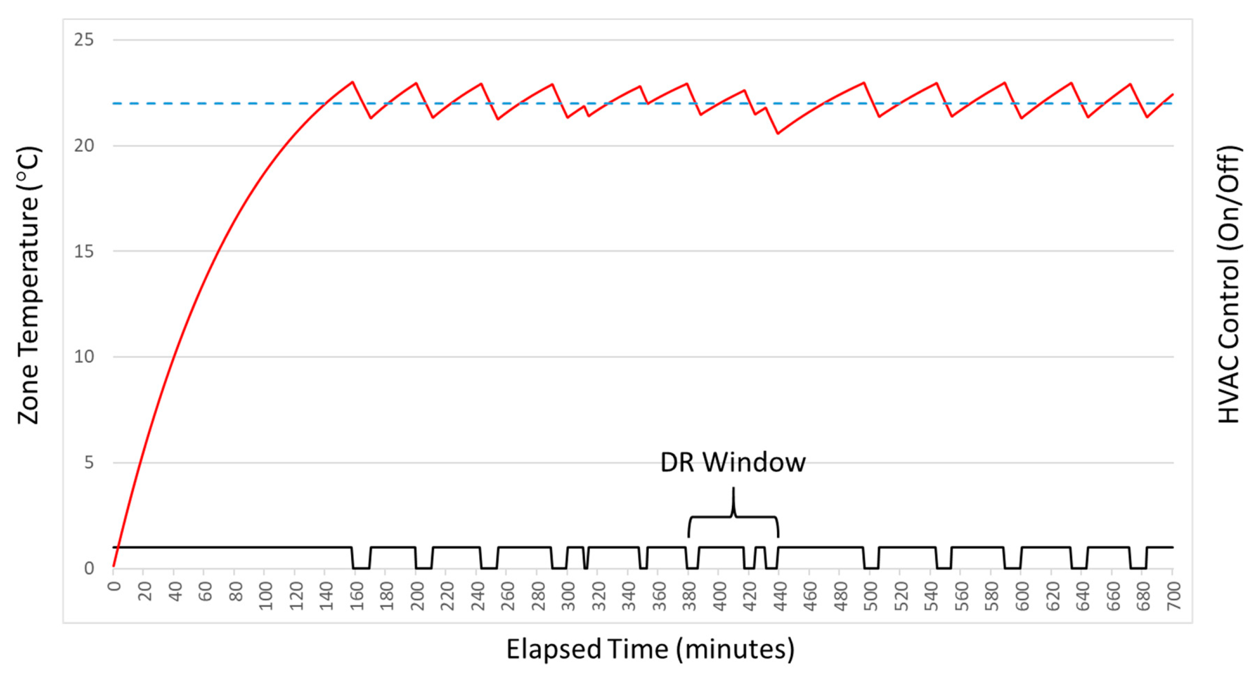
The first component of the objective function in Equation (4) is the sum of squared errors between the actual building temperature and its setpoint. A quadratic penalty term is appropriate as it approximately captures the relationship between temperature error and thermal comfort (see, e.g., [22]). During working hours, this will be typically 22.0 °C in winter and 24.5 °C in summer [22]. The second component is the sum of squared control moves weighted by the scalar term λ, which is used to suppress excessive switching of the controls. The indicator weights w(k) and bound U_U are used in combination to penalize electricity consumption during a specific defined window of the prediction horizon (corresponding to DR events). DR events are enabled for a particular stage by setting the indicator variable w(k) equal to ‘1’. As with all rolling horizon predictive control schemes, once the optimization has been solved for the current time step, only the first control (corresponding to u(k)) is applied. At time step k + 1, the process is repeated with repeated measurement information.

It is quite straightforward to see that for all but prediction horizons of one or two steps in length, and in the absence of any DR activity over the horizon (implying no constraint bounds in Equation (8)), then the control law resulting from the solution of Equations (4)–(7) is a switching surface dependent upon two factors. The first is the predicted difference between the reference temperature T_R(k + d) and actual temperature T(k + d) and the second is the previous state of the control input, u(k − d − 1). In this situation, the control defaults to a predictive relay-based controller with deadzone Δ ≈ √λ(k). In the presence of upcoming DR events, however, the effective switching surface can change considerably to provide optimal pre-heating (or cooling). In addition, the solution of the optimization problem contains useful predicted quantities regarding upcoming DR events. In particular, since the future control signals can only be ‘1’ or ‘0’, the predicted electricity consumption of the HVAC unit during any upcoming DR event—denoted as URC(k)—is easily derived from either inspection of the solution vector, or from the left hand side (l.h.s.) of constraint (8), as follows:

$$URC(k)=K_E\cdot T_s\cdot {\displaystyle \sum _{i=0}^{M-1}(u(k+i)\cdot w(k+i))}.$$

(9)

For upcoming DR events, the integer U_U on the right hand side (r.h.s.) of constraint (8) can be used to limit URC(k) and specify a load curtailment/reduced consumption from the HVAC unit. These observations will be exploited in the sequel, during which the DR allocation mechanism will be presented. The optimization problem of Equations (4)–(8) is easily formulated as a mixed-integer quadratic program (MIQP), or alternatively as an approximate mixed-integer linear program (MILP) [16,21]. In order to improve the run-time efficiency of the approach (and enable bounded worst-case execution times), the DP method is chosen. DP (see Bellman, [23]) is a computational method for solving optimal control problems with separable additive performance indices. It is based on the recursive application of Bellman’s ‘Principle of Optimality’ [23,24]:

‘An optimal policy has the property that whatever the initial state and the initial decision are, the remaining decisions must form an optimal policy with regard to the state resulting from the first decision.’

The mathematical form of this idea can be expressed as a backwards sequence featuring the solution of simpler optimization problems at each stage. Continuing backwards from the end stage N to the current stage k—and applying the principle of optimality at each stage—will result in the following recurrence relations for discrete DP [24]:

$$\begin{array}{l}{J}_N(x_N)=g_N(x_N);\\ k=N-1,N-2,...,1,0:\\ J_k(x_k)=\underset{u_k\in U_k(x_k)}{\min }\{g_k(x_k,u_k)+J_{k+1}(f_k(x_k,u_k))\};\end{array}$$

(10)

where J_k(x_k) is the cost of entering stage k with state x_k, g_k(x_k) is the cost for entering stage k with state x_k, U_k(x_k) is the set of allowed controls for the input u_k when the state x_k is entered at stage k, and f_k(x_k, u_k) is a function which maps the state x_k onto state x_k+1 when control u_k is applied at step k. In discrete DP (DDP), the state vector is mapped onto a grid of size S and the controls onto a grid of size U. By iterating through the recursion and trying all admissible control values at each admissible set of state values, a vastly reduced search space is explored when compared to a pure brute-force search; at the end of the minimization, a solution grid is obtained and the optimal control is obtained from the position in the grid corresponding to the current state. In the current context, the state variable is the temperature T(k) plus the previous applied control u(k − 1). The admissible controls are the current control u(k), having two possibilities (U = 2) at each stage in the absence of DR, but some possibilities may not be admissible if they invalidate constraint (8) when DR is active. In the approach taken in this paper, constraint (8) is translated into a penalty function inserted into the objective; with an iterative tightening of an applied weight upon constraint violation (a maximum of 10 iterations is employed). The temperature is mapped into a discrete grid of over a suitable working range, e.g., 10–30 °C; the control is already discrete in nature. The transition function f_k(x_k, u_k) is given by the linear Equation (6). In the case that the HVAC dynamics are actually non-linear, then this can easily be captured by an appropriate choice of transition function. During the recursion, the minimal cost function is stored for each admissible state along with the corresponding partial sum of the l.h.s of constraint (8). After the recursion, the value of UDR(k) is readily computable using Equation (9) and the final value of this partial sum. In many situations, temperature sensors either have 10-bit resolution—or can easily be cast or truncated into this range—giving a full state size S = 2¹¹. As the run-time complexity of the DDP algorithm is given by O(M.U.S), the algorithm runs efficiently even for a relatively large prediction horizon M, which may be needed for best results. During the backwards recursion, only the current and next stage costs and the partial l.h.s. of constraint (8) are actually required, reducing the memory requirement to O(U.S). As sampling time requirements of approximately one minute are sufficient in many instances (due to the comparatively slow thermal dynamics), then the algorithm is clearly suitable for deployment without undue problems in a small/low-cost embedded system.

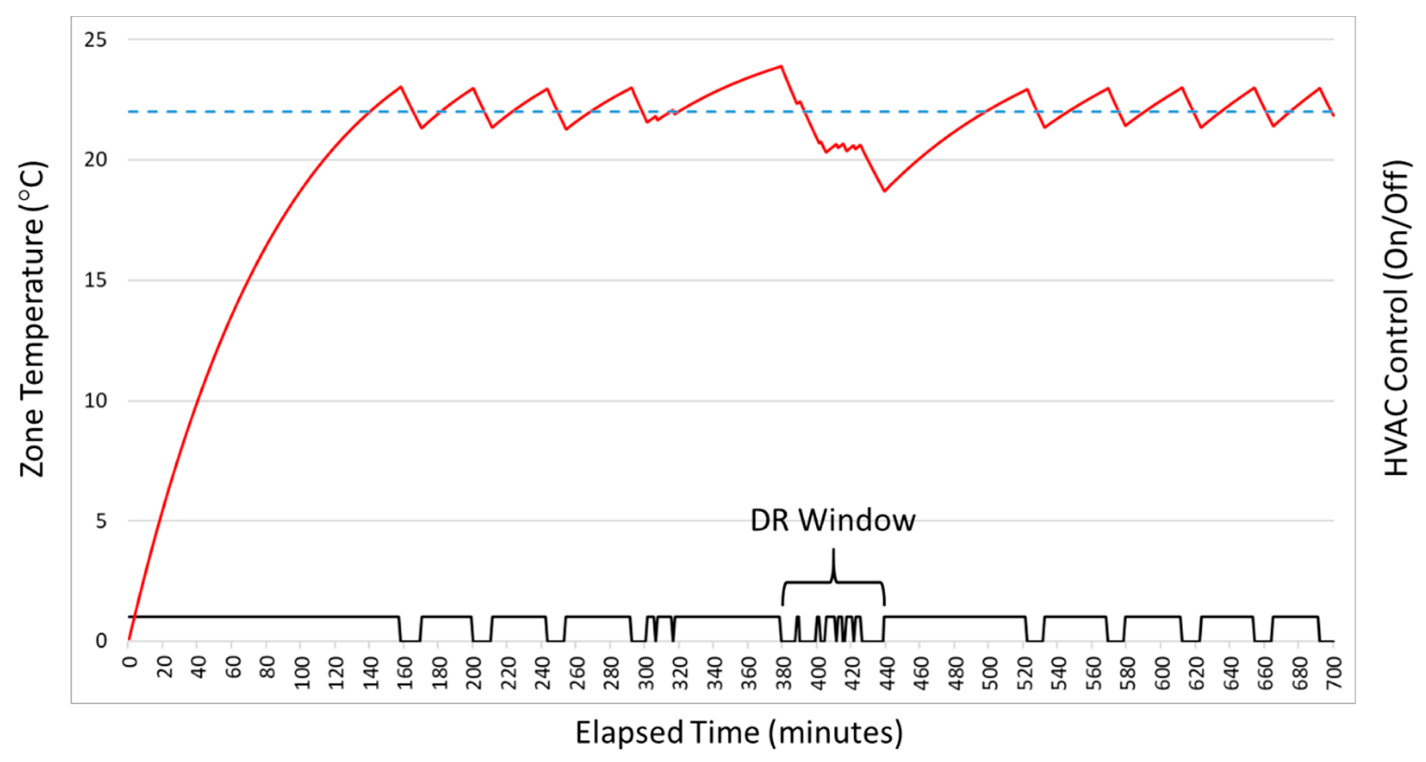
3.2. Generation of Predicted Baseline and Reduced Consumption

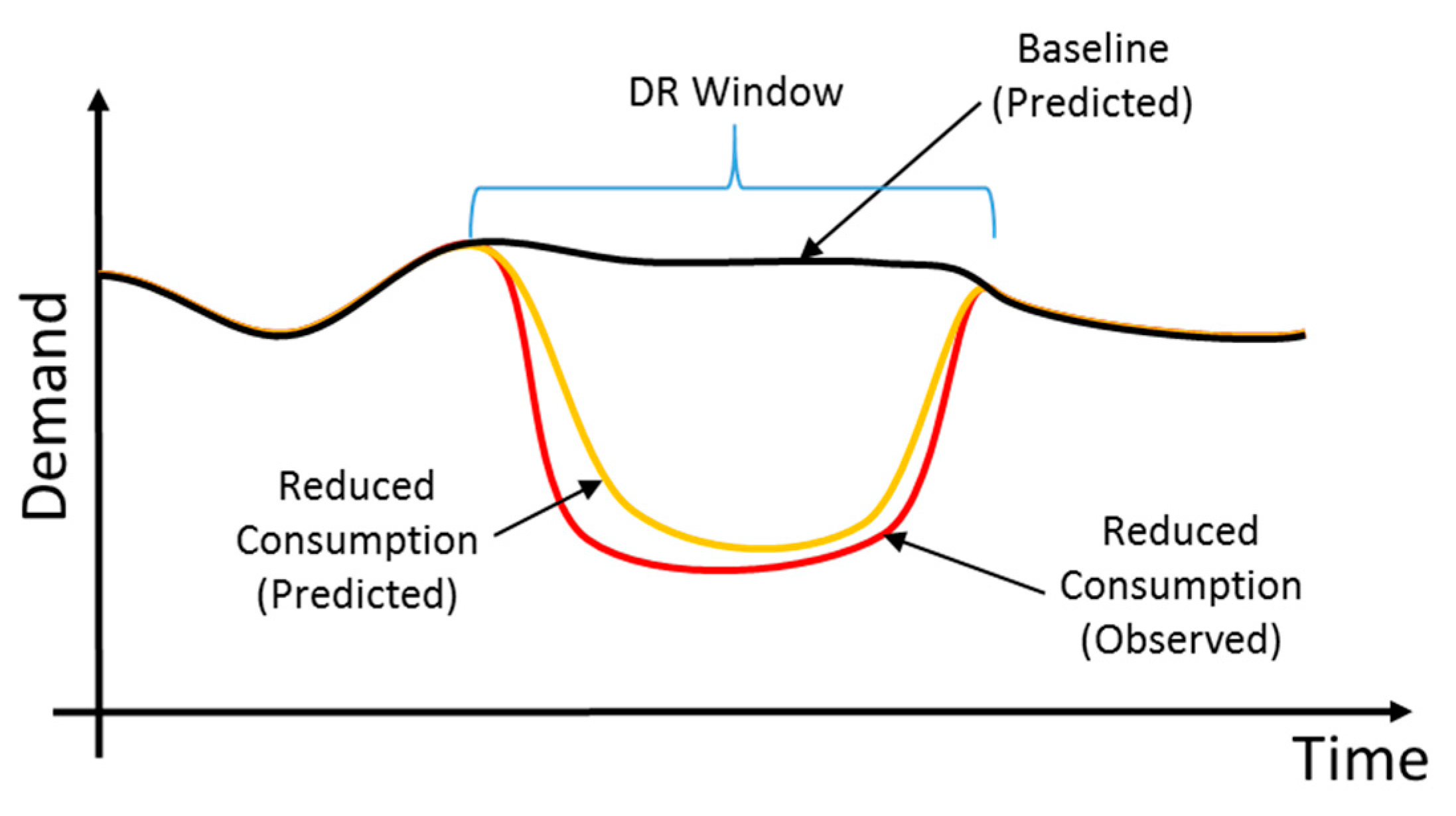
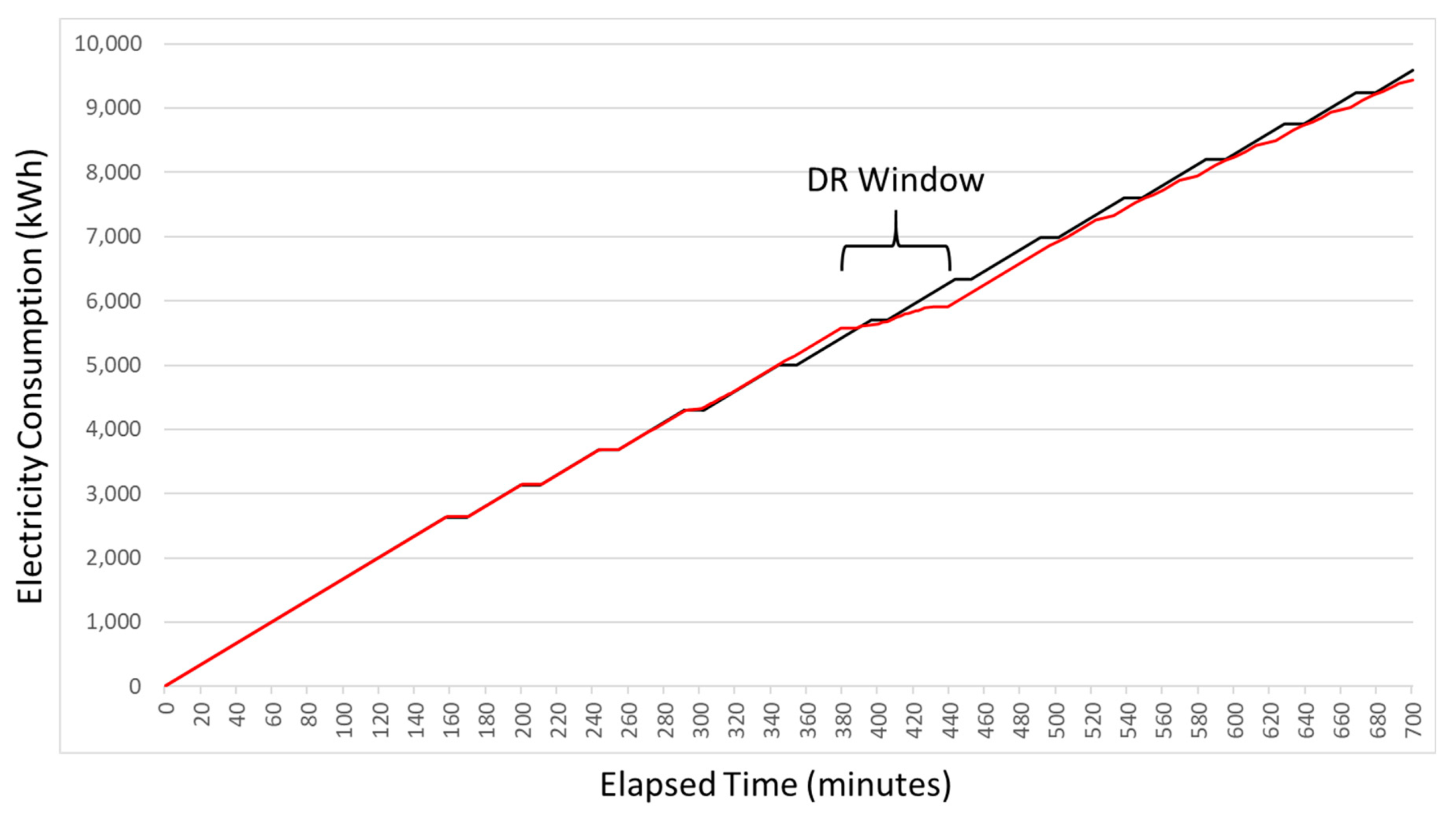
As discussed earlier, the effective practical implementation of a DR scheme requires the generation of both an accurate and reliable predicted baseline and an accurate and reliable predicted reduced consumption [25]. As shown in Figure 3, the baseline represents a counterfactual prediction (either forecast or backcast, generated on-line or off-line) of electricity consumption for targeted assets during the time-period corresponding to a DR event, under the assumption that no corrective DR action will be/had been taken. As also shown in Figure 3, the reduced consumption represents a prediction (forecast, generated on-line) of electricity consumption for targeted assets during the time-period corresponding to a DR event, under the assumption that corrective DR action will be taken. Note that although the observed reduced consumption in Figure 3 is always lower than predicted, this is not necessarily the case generally, and the accuracy of prediction depends heavily upon the models and methods employed.

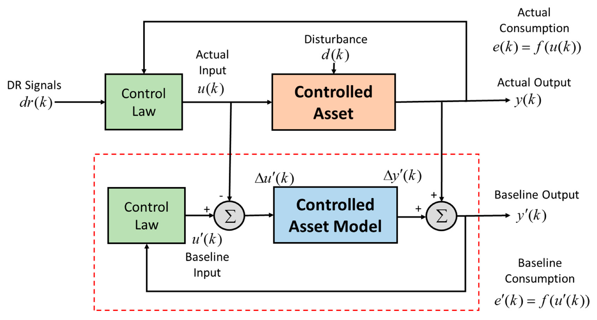
Both the predicted baseline and predicted reduced consumption are also dependent upon many factors including occupancy, ambient temperature and weather conditions, and it has proved a challenging and ongoing task to select suitable methods for their implementation [25]. The baseline consumption is needed to gauge performance of controlled assets during a DR event and for post-event financial settlement, where it is compared to the actual measured consumption. Therefore, the baseline should be accurate as possible. In the context of the research presented here, it is required to generate a reliable baseline across the rolling horizon for an HVAC unit in an on-line fashion. The methodology proposed is illustrated in Figure 4.

As can be seen in Figure 4, the controlled asset is driven by input u(k) and produces output y(k), and consumption E(k) is derived as a function of the input signal f(u(k)). The controlled asset is also driven by a disturbance sequence d(k) which impacts the output y(k); this sequence may consist of partially known (measured) values along with unmeasured or stochastic values. The asset input signal u(k) is generated by closed-loop feedback controls, which are also driven by external DR signals represented by r(k). The baseline is generated on-line (in real-time) by the components contained within the dashed red box; the asset model represents a discrete-time dynamic model of the controlled asset, while the asset model input signal u’(k) is given by the same closed-loop feedback algorithm which drives the actual controlled asset. However, the DR signals r(k) are suppressed from the control law in the baseline case to ensure the counterfactual sequence of inputs is generated. The baseline consumption sequence E’(k) is derived as a function of the baseline input signal f(u’(k)). Since the disturbances d(k) and plant-model mismatch can both impact upon the baseline accuracy, the counter-factual baseline output is generated on-line as follows. The actual nominal control input u(k) is first subtracted from the baseline input u’(k) to generate an input deviation signal Δu’(k), which acts as input to the asset model to produce an output deviation signal Δy’(k). The baseline output y’(k) is then produced by adding the deviation signal Δy’(k) to the measured output y(k). This ensures that the effects of disturbances and plant-model mismatch on the actual output y(k) are contained within the baseline output y’(k), which also captures the impact of the baseline control sequence u’(k) to ensure accuracy of the baseline. In the context of the current work, the controlled asset is the HVAC system, the controlled asset model is represented by Equation (2) with the measured part of the disturbance sequence being the ambient temperature, and the control law is the rolling-horizon non-linear MPC procedure given by Equations (4)–(8).

For the effective application of aggregated DR, it is required to generate both a predicted baseline and a predicted reduced consumption across the rolling horizon for each individual HVAC unit in an on-line fashion. At each timestep k, let the baseline consumption of the HVAC unit during an upcoming DR window be denoted as UBL(k) and the reduced consumption of the HVAC unit during an upcoming DR window be given as URC(k). Computation of this latter quantity as a by-product of the application of the DP algorithm was detailed in the previous Section. In order to compute the former quantity UBL(k), the DP algorithm can be applied to solve the optimization problem using baseline input u’(k) and output y’(k) as input data and setting constraint (8) r.h.s. U_U = ∞. As discussed in the previous section, the control law resulting from the solution of Equations (4)–(8) in the absence of any DR signals is a predictive relay-based controller. Therefore to simplify the process of generating the baseline controls u(k + i|k) and y(k + i|k) (i.e., i-step predictions of the asset input and output, incorporating measured disturbances such as weather forecast), Equation (3) may be employed at each stage with deadzone Δ = λ²/2. Thus, both quantities can be computed in a straightforward procedure integrating both unit DR controls and unit baseline/reduced consumption predictions in an ITU-based edge device.

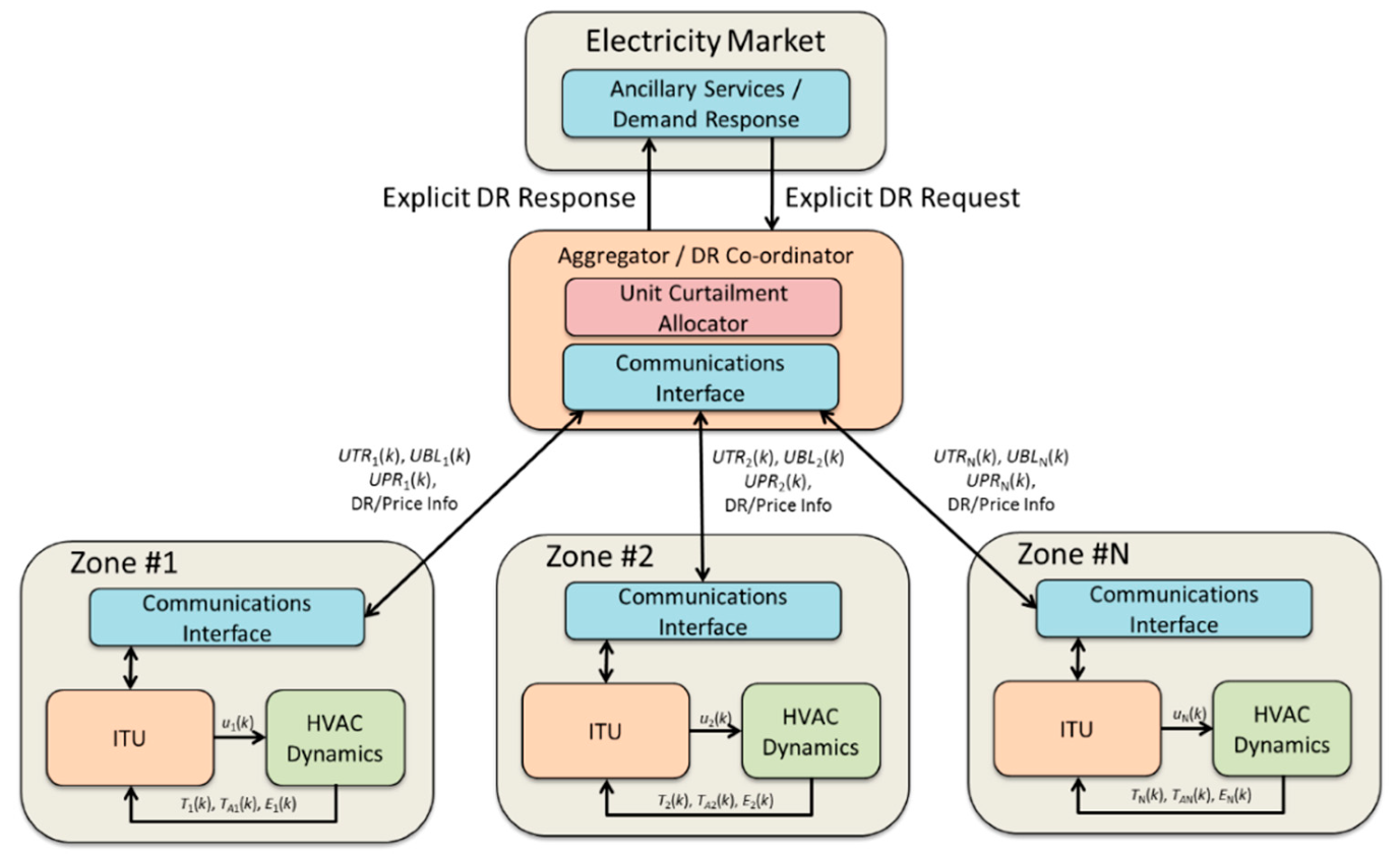
3.3. Coordinated Dispatch Scheme

Consider the arrangement of HVAC units (with their edge-based local dispatch optimizers) in the presence of a (cloud-based) aggregator at the network core, in the presence of a wider DR marketplace as shown in Figure 5. Assume that a flexible IP-based communications infrastructure is employed to interconnect the core and network edges (e.g., using Web Services, OpenADR protocol, etc.), and to provide loose synchronization of their clocks (e.g., using Network Time Protocol (NTP)).

For the aggregated DR coordination scheme, the following approach is employed. In a multiple-zone scenario, let the predicted electricity consumption at time step k for an upcoming DR event involving HVAC unit j be given as URC_j(k). Similarly, let the predicted baseline electricity consumption at time step k for an upcoming DR event involving HVAC unit j be given as UBL_j(k). This quantity is computable as detailed in the last section. Since for each HVAC unit j and for every time step k it must hold that UBL_j(k) ≥ URC_j(k) (i.e., the predicted unit baseline consumption is not less than the unit DR consumption during a DR event), at step k the explicit unit predicted reduction in load—denoted as UPR_j(k)—for an upcoming DR event is given by: UPR_j(k) = UBL_j(k) − URC_j(k). This quantity is easily computed in each ITU as detailed in the previous section. Then the predicted aggregated explicit reduction in load for an upcoming DR event at time step k—denoted APR(k)—for N participating HVAC units can be computed by the aggregator as:

$$APR(k)={\displaystyle \sum _{j=1}^{N}UP{R}_j(k)}.$$

(11)

Let the target aggregated electricity reduction consumption for an upcoming DR event be given as ATR(k) ≥ 0, and the target reduction in load for individual HVAC unit j be given as UTR_j(k). Since it has been assumed that the HVAC controls are binary in nature, in a given DR window the available load curtailment is limited between zero and the maximum available from the predicted baseline in discrete steps. As such, assume that each HVAC unit j ∊ N offers an agreed price-schedule for load curtailment X_j, such that a specific load L_j,l may be reduced for a price p_j,l by selecting one of l ∊ X_j different discrete price/curtailment options. Only one (or none) of the price/curtailment options can be selected for a given HVAC unit, for any given DR event. The objective for the DR coordinator is then to (i) at the start of a preparatory event, allocate individual HVAC unit load curtailments to meet the aggregate DR requirements; and (ii) should an HVAC unit opt-out or become unavailable—or environmental/pricing conditions otherwise change leading to an invalid initial allocation—reallocate curtailments to best suit the new conditions. The allocation/reallocation problem for N available units at time-step k can be written as a variant of a standard integer knapsack problem, as follows:

Minimize:

$${\displaystyle \sum _{j=1}^N{\displaystyle \sum _{l\in X_j}{p}_{j,l}{x}_{j,l}}}$$

(12)

subject to:

$${\displaystyle \sum _{j=1}^{N}UT{R}_j(k)}\ge ATR(k)$$

(13)

$$UT{R}_j(k)={\displaystyle \sum _{l\in X_j}{L}_{j,l}{x}_{j,l}},1\le j\le N;$$

(14)

$$UT{R}_j(k)\le UB{L}_j(k),1\le j\le N;$$

(15)

$${\displaystyle \sum _{l\in X_j}{x}_{j,l}\le 1},1\le j\le N;$$

(16)

$$x_{j,l}\in \left\{0,1\right\},1\le j\le N;l\in X_j.$$

(17)

where x_j,l ∊ {0, 1} are binary variables that indicate whether load reduction level L_j,l is active for HVAC unit j. Equation (12) defined the main objective, to minimize DR costs while meeting the target reduction in demand (constraint (13)). Constraint (14) allocates load reduction level to individual unit targets, while constraint (15) ensures that individual unit load reductions are not greater than the individual unit baselines for the upcoming event. Constraint (16) enforces mutual exclusion in the choice of load reductions to individual units based upon the available price/curtailment options for that unit. Note that the presence of this constraint allows that any costs for activating a particular HVAC unit for DR purposes can be added into the corresponding costs for discrete load curtailment. The presence of the constraints also suggests that the problem can be efficiently solved using standard DP techniques, using a slight variant of the standard knapsack DP approach [26]. The time and space complexity of this approach is O(N.D.X), where N is the number of participating units, D is the level of load curtailment requested and X is the largest cardinality of curtailment choices among the participating units [23,24]. Alternatively, efficient Branch-And-Bound techniques are known and can be applied [26]. Should the problem defined by Equations (12)–(17) prove infeasible, this will be due a violation of constraint (13), indicating that there is not enough capacity to achieve the aggregated DR value. In this case, either further units should be brought into the DR scenario, or the aggregator should report that it might not be able to deliver the required target to the market.

4. Evaluation

In this section, the design and results obtained from both a computational study and experimental test are reported in order to illustrate the proposed approach and to provide validation of its effectiveness in providing explicit DR in an aggregated environment.

4.1. Computational Study

For the computational study, five HVAC units are considered. The thermal dynamic model chosen for each unit represented a typical heating/cooling zone with thermal time constant ≈20 min, sized with a 200 kW direct expansion air conditioner heat pump. The dispatch algorithm was configured to have a setpoint of 22 °C and deadzone Δ = 1 °C. An ambient temperature profile was generated from recorded winter seasonal data in the UK in each simulation run, with the units configured for heating purposes. The five HVAC units offer DR reductions as follows: Four of the units (A–D) offer 0–100 kWh in 3.3 kWh steps @ 0.25€/kWh, and 103.3 kWh to 160 kWh in 3.3 kWh steps @ 0.35€/kWh EUR/kWh. The final unit (E) offers 0–160 kWh in 3.3 kWh steps @ 0.2€/kWh. The example considers the case of an aggregate load curtailment (STOR request) of 500 kWh being required for an event lasting one hour.

Application of the modified knapsack DP algorithm (Equations (12)–(17)) yields the simple minimum-cost solution as 160 kWh from HVAC unit E, 40 kWh from HVAC unit D and 100 kWh each from units A–C, giving the required 500 kWh at a total cost of €117. Four simulation runs were thus considered for an HVAC unit in the presence of the STOR event: (i) no DR activated (baseline); (ii) 40 kWh reduction through DR; (iii) 100 kWh reduction through DR; and (iv) 160 kWh reduction through DR. The responses obtained are given in Figure 6, Figure 7, Figure 8 and Figure 9. Each figure indicates zone temperature in °C (red trace), HVAC on/off status (black trace) and temperature setpoint in °C (dashed blue trace) plotted versus time, in minutes. The figures also indicate the location of the DR window on the time axis. The DR window commences after 380 min for a duration of 60 min; the notification of the upcoming DR event occurs after 140 min.

In the baseline case, with zero DR activity, after initially heating to the setpoint the temperature cycles ±1 °C around the setpoint, and continues to do so during the DR window, with the HVAC unit operating as normal. After initially achieving setpoint, the maximum, minimum and average temperatures recorded were 23.0, 21.2 and 22.2 °C respectively. In this case, 160 kWh is consumed during the DR window. In the 40 kWh STOR case, after initially heating to the setpoint the temperature again starts to cycle ±1 °C around the setpoint; but after approximately 290 min, deviations from the regular cycle can be observed as the unit prepares for DR activity during the DR window. After initially achieving setpoint, the maximum, minimum and average temperatures recorded were 23.0, 20.6 and 22.1 °C respectively. In this case, 120 kWh is consumed during the DR window. Focusing now upon the 100 kWh STOR case, after initially heating to the setpoint the temperature again starts to cycle ±1 °C around the setpoint. After approximately 290 min, deviations from the regular cycle can be observed as the unit prepares for DR activity during the DR window, during which 60 kWh is consumed. A distinct period of pre-heating can be observed prior to this window. After initially achieving setpoint, the maximum, minimum and average temperatures recorded were 23.9, 18.7 and 22.0 °C respectively. Finally, concerning the 160 kWh STOR case, the unit again starts to cycle the temperature ±1 °C around the setpoint after initially heating. A pronounced period of pre-heating begins at the 260-min mark as the unit prepares for DR activity during the DR window. In this case, zero kWh is consumed during the DR window, i.e., the unit remains in the ‘off’ state. After initially achieving setpoint, the maximum, minimum and average temperatures recorded were 24.5, 16.1 and 21.7 °C respectively.

As can be observed in Figure 8 and Figure 9, the proposed dispatch strategy is effective in producing the DR actions required in order to surgically reduce consumption during DR events. Although this has some negative impact upon the zone temperature, this impact is minimized through the optimization which has been developed. Accurate baselining and optimal activation of the unit both prior to and during the DR window itself are evident. Figure 10 plots the electricity consumption (in kWh) for all five HVAC units over the duration of the simulation time in both the DR and no DR (baseline) cases. The aggregated consumption for the no-DR case during the DR window was found to be 833.3 kWh, while the aggregated consumption for the DR case during DR window was found to be 333.3 kWh. The commanded reduction of 500 kWh has clearly been achieved, and an accurate baseline provided for settlement purposes. Figure 6, Figure 7, Figure 8, Figure 9 and Figure 10 also clearly indicate that consumption has been shifted away from the DR window to occur both before and after the window itself.

4.2. Experimental Evaluation

For the experimental evaluation, testing was performed at an experimental site on the Teesside University campus in Middlesbrough, UK, within the context of the Demand Response in Blocks of Buildings (DR-BoB) Horizon 2020 project. The experiment was undertaken on four HVAC/AHU (air handling units) providing both heating and cooling services to a large building housing office spaces and lecture rooms. Figure 11 shows a photograph of the locations on the rooftop at the demonstration site building. The units were configured to operate in cooling mode, with circulating water setpoint set at 5.25 °C with deadzone Δ = 1.25 °C. The cooled water feeds into individual room heat exchangers to provide air conditioning and cooling in the office spaces and lecture rooms.

To provide remote override and operation of the HVAC controls, and provide an interface to measured temperatures, a BACNet connection to an additional programmable control device was employed. This device represented the ITU, and allowed the implementation of the dispatch controls. An internet connection to a cloud-based coordination application sending the simulated DR signals was also implemented over a secured public IP connection. The HVAC dynamics are non-linear in the HVAC units, being partially dependent upon the thermal demand. This demand is predictable and manifests as a time varying coefficient a(k) in Equation (2). In addition, a small transmission zero is present and was included in the model, which provides a very good fit (≈90%) to historic recorded data. The experimental test was carried out on the afternoon of the 1st of September 2017, during which a DR event requiring a reduction of 200 kWh was simulated between the hours of 12:30 and 15:30. Results for the response of HVAC/AHU #1 are shown in Figure 12 and Figure 13. Figure 12 displays the chiller return temperature (in °C) for the unit during the course of the day, with the actual temperature displayed in red and baseline temperature displayed in black. The ambient temperature outside the building is displayed in green and the setpoint in blue. The unit is activated at approximately 09:30 and the water temperature is brought towards the setpoint. The disturbance at approximately 10:00 is best attributed to a load change as internal heat exchangers are switched on as the building becomes occupied. Pre-cooling of water temperature begins at 12:00 prior the DR event itself. The electricity consumption of the unit is shown Figure 13. The red trace displays the actual (metered) consumption of the unit, while the black trace displays the baseline (counterfactual) consumption of the unit. Figure 12 and Figure 13 show evidence of pre-cooling, and the generation of an accurate baseline indicating a post-event reduction in electricity consumption from the unit of 54.13 kWh. The overall aggregated reduced consumption obtained from HVAC units #2, #3 and #4 were at similar levels, meeting the aggregated target of 200 kWh. Overall, these results provide a practical, experimental and real-world validation of the techniques described in this research.

5. Conclusions

This paper argues that since energy consumption is estimated to be about 40% accountable to buildings, sustainable demand side management is one possibility to mitigate the dependence of buildings on the electrical grid. As such, a novel approach to coordinated demand response (DR) for aggregated HVAC is presented to support surgical (explicit) DR in buildings and blocks or groups of buildings, which are possibly spread across multiple geographic locations. This approach presents a large-scale decentralized optimization framework that leverages concepts of Industry 4.0, incorporating distributed DP solutions for individual unit dispatch with a centralized DP allocation procedure. In addition, an accurate baselining procedure to enable effective calculation of reduced consumption and post-event settlement at the individual unit level has been proposed. The approach has been validated using calibrated simulation studies and experimental tests, and it is demonstrated that surgical DR can be effected by a number of coordinated units. Future work includes further representative testing of the proposed approach and its commercialization. In addition, future work will also investigate the integration of other forms of DR assets (e.g., combined heat and power (CHP) plant [27] and smart home appliances [28] under rolling-horizon techno-economic optimization) into the aggregated DR framework.

References

1. Isaksson, A.J.; Harjunkoski, L.; Sand, G. The impact of digitalization on the future of control and operations. Comput. Chem. Eng. 2018, 114, 122–129. [Google Scholar] [CrossRef]
2. Mahdavinejad, M.S.; Rezvan, M.; Barekatain, M.; Adibi, P.; Barnaghi, P.; Sheth, A.P. Machine learning for internet of things data analysis: A survey. Digit. Commun. Netw. 2018, 4, 161–175. [Google Scholar] [CrossRef]
3. Perez-Lombard, L.; Ortiz, J.; Pout, C. A review on buildings energy consumption information. Energy Build. 2008, 40, 394–398. [Google Scholar] [CrossRef]
4. Crosbie, T.; Short, M.; Dawood, M.; Charlesworth, R. Demand response in blocks of buildings: Opportunities and requirements. J. Entrep. Sustain. Issues 2017, 4, 271–281. [Google Scholar] [CrossRef]
5. Arteconi, A.; Polonara, F. Demand side management in refrigeration applications. Int. J. Heat Technol. 2017, 35, S58–S63. [Google Scholar] [CrossRef]
6. Proffitt, E. Profiting from Demand Side Response; Technical Publication; The Major Energy Users’ Council in Association with National Grid: London, UK, 2016. [Google Scholar]
7. Shi, Q.; Li, F.; Hu, Q.; Wang, Z. Dynamic demand control for system frequency regulation: Concept review, algorithm comparison, and future vision. Electr. Power Syst. Res. 2018, 154, 75–87. [Google Scholar] [CrossRef]
8. Luo, F.; Ranzi, G.; Dong, Z. Rolling horizon optimization for real-time operation of thermostatically controlled load aggregator. J. Mod. Power Syst. Clean Energy 2017, 5, 947–958. [Google Scholar] [CrossRef]
9. Williams, S.; Short, M.; Crosbie, T. On the use of thermal inertia in building stock to leverage decentralised demand side frequency regulation services. Appl. Therm. Eng. 2018, 133, 97–106. [Google Scholar] [CrossRef]
10. Ramanathan, B.; Vittal, V. A framework for evaluation of advanced direct load control with minimum disruption. IEEE Trans. Power Syst. 2008, 23, 1681–1688. [Google Scholar] [CrossRef]
11. Hao, H.; Sanandaji, B.; Poolla, K.; Vincent, T.L. Aggregate flexibility of thermostatically controlled loads. IEEE Trans. Power Syst. 2015, 30, 189–198. [Google Scholar] [CrossRef]
12. Vrettos, E.; Anderson, G. Combined load frequency control and active distribution network management with thermostatically controlled loads. In Proceedings of the IEEE International Conference on Smart Grid Communications (SmartGridComm), Vancouver, BC, Canada, 21–24 October 2013. [Google Scholar]
13. Mathieu, J.L.; Koch, S.; Callaway, D.S. State estimation and control of electric loads to manage real-time energy imbalance. IEEE Trans. Power Syst. 2013, 28, 430–440. [Google Scholar] [CrossRef]
14. Wang, H.; Meng, K.; Luo, F.; Dong, Z.Y.; Verbič, G.; Xu, Z.; Wong, K.P. Demand response through smart home energy management using thermal inertia. In Proceedings of the Australia Universities Power Engineering Conference (AUPEC 2013), Hobart, TAS, Australia, 29 September–3 October 2013. [Google Scholar]
15. Luo, F.; Zhao, J.; Wang, H.; Wang, H.; Tong, X.; Chen, Y.; Dong, Z.Y. Direct load control by distributed imperialist competitive algorithm. J. Mod. Power Syst. Clean Energy 2014, 2, 385–395. [Google Scholar] [CrossRef]
16. Drgona, J.; Klauco, M.; Kvasnica, M. MPC-based reference governors for thermostatically controlled residential buildings. In Proceedings of the IEEE 54th Annual Conference on Decision and Control (CDC 2015), Osaka, Japan, 15–18 December 2015. [Google Scholar]
17. Callaway, D.S. Tapping the energy storage potential in electric loads to deliver load following and regulation, with application to wind energy. Energy Convers. Manag. 2009, 50, 1389–1400. [Google Scholar] [CrossRef]
18. Zhou, L.; Li, Y.; Wang, W.; Hu, X. Provision of supplementary load frequency control via aggregation of air conditioning loads. Energies 2015, 8, 14098–14117. [Google Scholar] [CrossRef]
19. Afram, A.; Janabi-Sharifi, A. Review of modelling methods for HVAC systems. Appl. Therm. Eng. 2014, 67, 507–519. [Google Scholar] [CrossRef]
20. Mathews, E.; Richards, P.; Lombard, C. A first-order thermal model for building design. Energy Build. 1994, 21, 133–145. [Google Scholar] [CrossRef]
21. Camacho, E.F.; Bordons, C. Model Predictive Control, 2nd ed.; Springer: Berlin, Germany, 2004. [Google Scholar]
22. Djongyang, N.; Tchinda, R.; Njomo, D. Thermal comfort: A review paper. Renew. Sustain. Energy Rev. 2010, 14, 2626–2640. [Google Scholar] [CrossRef]
23. Bellman, R.E. Dynamic Programming; Princeton University Press: Princeton, NJ, USA, 1957. [Google Scholar]
24. Bertsekas, D.P. Dynamic Programming and Optimal Control; Athena Scientific: Belmont, MA, USA, 2005. [Google Scholar]
25. Chelmis, C.; Aman, S.; Saeed, M.R.; Frincu, M.; Prasanna, V.K. Estimating reduced consumption for dynamic demand response. In Proceedings of the AAAI Workshop on Computational Sustainability, Austin, TX, USA, 1 April 2015. [Google Scholar]
26. Martello, S.; Toth, P. Knapsack Problems: Algorithms and Computer Implementations; John Wiley and Sons: Hoboken, NJ, USA, 1990. [Google Scholar]
27. Short, M.; Crosbie, T.; Dawood, M.; Dawood, N. Load forecasting and dispatch optimization for decentralized co-generation plant with dual energy storage. Appl. Energy 2017, 186, 304–320. [Google Scholar] [CrossRef]
28. Ogwumike, C.; Short, M.; Abugchem, F. Heuristic optimization of consumer electricity costs using a generic cost model. Energies 2016, 9, 6. [Google Scholar] [CrossRef] [Green Version]
29. Short, M. Optimal HVAC dispatch for demand response: A dynamic programming approach. In Proceedings of the International Conference on Innovative Applied Energy (IAPE’19), Oxford, UK, 15 March 2019. [Google Scholar]
Figure 1. Demand response concept.
Energies 12 04320 g001
Figure 2. Timeline of events in a short term operating reserve (STOR) demand response (DR) event.
Energies 12 04320 g002
Figure 3. Concept of predicted baseline, predicted reduced consumption and reduced consumption.
Energies 12 04320 g003
Figure 4. Methodology for online baseline generation.
Energies 12 04320 g004
Figure 5. Arrangement of actors and signal exchanges in the coordinated dispatch scheme.
Energies 12 04320 g005
Figure 6. Baseline STOR scenario (red trace, temperature; black trace, HVAC control).
Energies 12 04320 g006
Figure 7. The 40 kWh reduction STOR scenario (red trace, temperature; black trace, HVAC control).
Energies 12 04320 g007
Figure 8. The 100 kWh reduction STOR scenario (red trace, temperature; black trace, HVAC control).
Energies 12 04320 g008
Figure 9. The 160 kWh reduction STOR scenario (red trace, temperature; black trace, HVAC control).
Energies 12 04320 g009
Figure 10. Electricity consumption in kWh (red trace, DR case; black trace, baseline case).
Energies 12 04320 g010
Figure 11. Photograph indicating positioning of the four HVAC units at the demonstration site.
Energies 12 04320 g011
Figure 12. Recorded temperatures in °C (red trace, DR case; black trace, baseline case; green trace, ambient temperature).
Energies 12 04320 g012
Figure 13. Electricity consumption in kWh (red trace, DR case; black trace, baseline case).
Energies 12 04320 g013