Markov Chain Simulation of Coal Ash Melting Point and Stochastic Optimization of Operation Temperature for Entrained Flow Coal Gasification

Abstract

In the entrained flow coal gasification process, the gas production is critically affected by the operating temperature (OT) and coal ash melting point (AMP), and the AMP is one of key factors for the determinations of OT. Considering the fact that coal is a typical nonhomogeneous substance and the coal ash composition varies from batch to batch, this paper proposes the application of the Markov Chain (MC) method in simulation of the random AMP series and the stochastic optimization of OT based on MC simulation for entrained flow coal gasification. The purpose of this paper is to provide a more accurate optimal OT decision method for entrained flow coal gasification practice. In this paper, the AMP was regarded as a random variable, and the random process method, Markov Chain, was used to describe the random AMP series of feed coal. Firstly, the MC simulation model about AMP was founded according to an actual sample data, 200 sets of AMP data from an industrial gasification plant under three simulation schemes (the sample data were individually divided into 16, eight and four state groups,). The comparisons between the simulation results and the actual values show that the founded MC simulation model descries the AMP series very well. Then, a stochastic programming model based on MC simulation for OT optimization was developed. Finally, this stochastic programming optimization model was optimized by genetic algorithm (GA). Comparing with the conventional OT optimization method, the proposed stochastic OT optimization model integrated MC simulation can ascertain a more accurate OT for guiding the coal gasification practice.

1. Introduction

Coal is the most wildly used natural energy resource with the largest reserves. Compared with other energy sources, the utilization of coal has attracted wider attention in view of the advantages of wide distribution and easy exploitation of coal. In recent years, the increasing environmental and health concerns in utilization of coal promote the emergence of clean coal technologies [1,2,3,4]. Among the clean coal technologies, coal gasification is regard as a promising utilization of coal because of its low technology cost and high conversion rate [5]. In the coal gasification practice, the basic equipment can be grouped into three main categories: fixed bed gasifiers, fluidized bed gasifiers and entrained flow gasifiers [6,7]. Differ from fixed bed and fluidized bed gasification, entrained flow gasification operates at a higher temperature (above the melting temperature of ash) with smaller particles and produces high quality syngas with low methane and free tar content. In addition, this type of coal gasification has some advantages such as high carbon conversion, large production capacity, high thermal efficiency and a low environmental pollution [8,9]. On the contrary, there are also some disadvantages to be improved in entrained flow gasification such as slagging and fouling.

Because the ash discharging mode for entrained-flow bed gasifiers is liquid slagging, the melting characteristics of coal ash is a key factor influencing the gasifier operation [10]. Thus, the ash melting point (AMP) of the feed coal is an important reference index for the determination of operational temperature (OT), which is a critical parameter for the stable and efficient operation of the gasifier. When the temperature in a gasifier is lower than the AMP of the feed coal, the gasification reaction as well as coal conversion rate will be greatly reduced [11]. On the contrary, when the gasification temperature is far higher than the AMP, the ash in the coal may agglomerate, resulting in a reduction of the reaction contact between the gasifying agent and coal and an uneven air flow in the gasifier, which is not conducive to good gasification reactions [12]. Thus, the OT of the gasifier should usually be moderately higher than the AMP of the feed coal so as to facilitate the melting and flow of coal ash and maintain the gasification reaction [13]. Therefore, the AMP of feed coal is always paid special attention to in practice due to the important role it plays in the determination of the optimum OT for the gasification process.

Over the past years, in order to study the melting behavior of coal ash in gasifiers, many studies about the AMP of coal have been reported. Current studies on AMP of coal can be roughly divided into two categories: (i) the mechanism models that are based on the mechanism of chemical reactions; (ii) the empirical models that are based on data statistics. A large number of researchers have developed mechanism models in their studies on AMP of coal, for example, Chakravarty et al. [14], Dai et al. [15], Weber et al. [16], Kim et al. [17]. However, the mechanism models are very theoretical, with many assumptions, so the reaction process expressed by these formulas may deviate from the actual reaction process due to these assumptions. As for the empirical models for coal AMP, studies on this subject have developed rapidly and a great deal of literature on this subject has been published in recent years. Some statistic method such as linear and non-linear regression methods, as well as some advanced intelligent algorithms [18] such as artificial neural network(ANN), support vector machine (SVM), etc. were employed in these models. For instance, Ozbayoglu et al. [19] applied linear regression and non-linear regression, respectively, to the chemical composition of coal ash and the temperature of AMP for Turkish lignite. In [10,20,21,22], the authors took a large number of parameters of coal ash as training samples and used ANN to predict the AMP of different coals. In [23,24,25], the authors all took ash composition as input and AMP as output to build prediction models of AMP using SVM. Compared with the mechanism model, the advantage of the empirical models is that they avoid complex mechanism process analysis, and they can just extract information from historical data to predict the AMP of coal. Both the mechanism models and the empirical models have contributed to the study of ash problems (such as slagging and fouling), however, these models are static models, that is, the foundations for modelling are based on a point in time rather than a time series perspective. More importantly, these studies focus on the prediction of AMP based on the characteristics of coal rather than OT optimization based on dynamic AMP.

As one of the critical factors influencing the stable and efficient operation of a gasifier as well as the quality of gasification product, OT has always been one of the key parameters discussed in many entrained flow coal gasification studies, and its optimization is usually an important topic in a large number of published studies. For instance, Chen et al. [26] carried out some orthogonal designs to optimize some operating parameters of an entrained flow gasifier for coal-biomass co-gasification. As an important operating parameter, OT was optimized according to Taguchi’s philosophy. Vejahati et al. [27] optimized three operating variables, including OT, for a coal-coke gasification in an entrained flow gasifier using response surface methodology (RSM). In addition to the experiment-based studies, many researchers also discussed the temperature optimization in their simulation-based researches. Emun et al. [28] used Aspen Plus to study the effect of different operating variables on thermal efficiency. As a result, the optimal OT was 1550 °C with the highest thermal efficiency. Biagini et al. [29] developed an entrained-flow gasifier model in Aspen Plus, and obtained the optimal operating conditions including temperature through parametric analysis. Chen et al. [30] applied a computational fluid dynamics (CFD) simulation method to develop an optimization analysis procedure of the gasification process in an entrained-flow gasifier, and obtained a best temperature of 1227 °C. Shastri et al. [31] developed a CFD model for a single-stage coal gasifier. Eleven parameters including OT were stochastically optimized by using the parameter space investigation method. Wei et al. [32] used the iterative adaptive dynamic programming (IADP) method to establish a nonlinear optimization control scheme for the coal gasification system. They concluded that the optimal OT should be controlled at around 1320 °C. Actually, the composition of pulverized feed coal varies from batch to batch, and even in the same batch of pulverized coal, there may be fluctuations in composition depending on the feeding time. In turn, the AMP of feed coal usually manifests as a dynamic series over a period of time. Thus the target of OT optimization is actually to seek an optimal OT that is best adapted to the dynamic changes in coal composition from batch to batch and extending to the dynamic changes in AMP. However, in reviewing the current studies on OT optimization, a lot of the reported studies involve static optimization because they are mainly based on static small-scale experiments or simulation experiments and the dynamic changes in coal composition as well as in AMP series of feeding coal are not taken into account.

In this paper, the AMP of feed coal over a period of time is treated as a group of random data series based on random perspective. A stochastic process theory, Markov Chain (MC), is used to simulate and describe the AMP series. A Markov process is a stochastic process model describing a sequence of possible events that satisfies the Markov property. In the philosophy of MC, the probability of each event depends solely on the state attained in the previous event, and this dependence obeys a certain probability distribution [33]. MC models can express the dynamic changes of a random series and predict the future changes of the system through the transition probability of state change among different variables. Because of the clear mathematical meaning of the MC model, it is widely used in modelling or simulation for different applications. For example, Afzal et al. [34] established a hidden Markov model that solves the problem of information prediction in industrial process control. Reference [35] provided a general approximation framework for (path-dependent) option evaluation under time-varying Markov processes. Reference [36] applied the Markov decision process to the control of the hybrid energy storage system, increasing the self-consumption of photovoltaics by 5%. In [37], a semi-Markov process was used to describe the machine degradation process, and a fault detection scheme based on Bayesian estimation was proposed to achieve more effective early fault detection. Others similar reports can be found in [38,39,40,41]. Recently, there have been a few reports about the application of MC in coal gasification. References [42,43] introduced a residence time distribution model of the granular phase in a gasifier based on MC. The results showed that the simulation results are basically in agreement with the measured data, which can be used to predict the residence time distribution of granular phase in the gasifier. However, to our best knowledge, there no studies on the utilization of MC in the simulation of AMP of coal, especially studies on OT optimization based on MC simulation for entrained flow coal gasification process have been reported so far.

The purpose of this paper is to describe our study on: (i) using MC to simulate the AMP series of feed coal for an entrained flow gasification process, (ii) stochastic program modelling based on MC simulation of AMP for OT optimization, and (iii) solving OT optimization with a genetic algorithm (GA). In this study, the AMP series of a feed coal was regarded as a random series, and the simulation for the AMP series with MC was carried out based on 200 sets of actual AMP data collected from an industrial gasification plant. Then a stochastic programming model with the target of optimizing OT based on MC simulation was proposed. Finally, the optimal OT was ascertained by solving the stochastic programing model using GA.

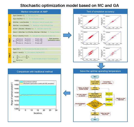
2. Simulation Approach for AMP Series

2.1. Marckov Chain

The Markov chain is a modeling and prediction method that works based on a stochastic process in order to describe a series of uncertain events [33]. In this type of stochastic process, the Markov property that the future prediction of a process variable could be made independent of the process history should be satisfied. For a stochastic process $\left\{X_t,t=0,1,2,\dots \right\}$ with a finite number of possible values, the statement that $X_t$ being equal to i expresses that the process is in state i when the time is at t. Figure 1 shows the state transition of a MC process. For a given past state $X_0,X_1,\dots ,X_{t-1}$ and the present state $X_t$, the condition distribution of the future state $X_{t+1}$ is independent of the past state and depends only on the present state. As shown in Figure 1, state set $S=\left\{1,2,\dots ,i,j,\dots n\right\}$, and the state transition with non-aftereffect property can be achieved by a fixed possibility of $P_{ij}$ [44]:

$$\begin{array}{l}P\left\{X_{t+1}=j|X_t=i_t,\dots ,X_1=i_1,X_0=i_0\right\}\hfill \\ =P\left\{X_{t+1}=j|X_t=i_t\right\}\hfill \\ =P_{ij}\hfill \end{array}$$

(1)

where $P_{ij}$ indicates the probability of a process being transferred to state $X_{t+1}$ at the time of state $X_t$.

$P_{ij}$ should satisfy the following conditions:

$$\begin{array}{l}{\sum }_{j=1}^n{P}_{ij}=1\hfill \\ P_{ij}\ge 0,\hfill \\ i,j=1,2,\dots ,n\hfill \end{array}$$

(2)

where $n$ is the total number of states. Then the Markov characteristic of a data series could be expressed by a matrix of transition probability $\mathit{P}$:

$$\mathit{P}=\left[\begin{array}{cccc}{P}_{11}& P_{12}& \cdots & P_{1n}\\ P_{21}& P_{22}& \cdots & P_{2n}\\ ⋮& ⋮& \ddots & ⋮\\ P_{n1}& P_{n2}& \cdots & P_{nn}\end{array}\right]$$

(3)

Matrix $\mathit{P}$ (Equation (3)) is the first order one-step transition matrix. In matrix P, the ith row, vector V, represents the one-step transition probability of state $i$. Then the n-step transition probability vector of state $i$ could be expressed by the following formula:

$${\mathit{V}}_i^n={\mathit{V}}_i{\mathit{P}}^{n-1}$$

(4)

As the embedded Markov chain is assumed ergodic, the stationary distribution, described by an k-element vector $\mathbf{\pi }$ [45], can be obtained solving the following system of linear equations:

$$\{\begin{array}{c}\mathbf{\pi }\mathit{P}=0\\ {\sum }_{i=1}^n{\mathbf{\pi }}_i=1\end{array}$$

(5)

where the last equation specifies the normalization of the probability distribution.

2.2. MC Simulation Procedure for AMP

The state transition probability matrix P is the core of Markov theory. The n-dimensional state transition probability matrix can be used to describe the change rule of any state in the stochastic system, which greatly simplifies the complexity of the stochastic model. Thus, Markov theory has been widely used in stochastic modelling.

In this paper, a MC simulation for 200 sets of AMP data (see Appendix A

Table A1. Simulation data and sample data deviation in three cases (the sample data of coal is from Hebi lean coal).

SerialNumber	Sample Data/°C	Simulated Data/°C			Absolute Deviation/°C			Relative Deviation
		Case I	Case II	Case III	Case I	Case II	Case III	Case I	Case II	Case III
Training set
1	1386.73	1389.71	1382.70	1369.38	2.98	4.03	17.35	0.21%	0.29%	1.25%
2	1348.07	1354.56	1335.43	1353.52	6.49	12.64	5.45	0.48%	0.94%	0.40%
3	1358.40	1351.29	1368.33	1332.41	7.11	9.93	25.99	0.52%	0.73%	1.91%
4	1351.90	1359.78	1341.63	1339.37	7.88	10.27	12.53	0.58%	0.76%	0.93%
5	1341.64	1355.24	1340.72	1358.78	13.60	0.92	17.14	1.01%	0.07%	1.28%
6	1339.47	1339.87	1348.71	1320.35	0.40	9.24	19.12	0.03%	0.69%	1.43%
7	1337.02	1327.97	1343.08	1319.99	9.05	6.06	17.03	0.68%	0.45%	1.26%
8	1363.06	1358.19	1354.76	1344.43	4.87	8.30	18.63	0.36%	0.61%	1.38%
9	1342.80	1345.99	1338.90	1332.40	3.19	3.90	10.40	0.24%	0.29%	0.77%
10	1337.50	1334.19	1324.86	1322.72	3.31	12.64	14.78	0.25%	0.94%	1.09%
11	1347.74	1339.69	1357.57	1357.87	8.05	9.83	10.13	0.60%	0.73%	0.75%
12	1341.27	1342.88	1331.90	1356.87	1.61	9.37	15.60	0.12%	0.69%	1.16%
13	1348.54	1356.14	1344.16	1363.90	7.60	4.38	15.36	0.56%	0.32%	1.14%
14	1325.90	1329.68	1333.87	1345.15	3.78	7.97	19.25	0.29%	0.59%	1.43%
15	1334.57	1340.74	1329.23	1316.11	6.17	5.34	18.46	0.46%	0.40%	1.37%
16	1350.79	1350.08	1356.87	1367.46	0.71	6.08	16.67	0.05%	0.45%	1.24%
17	1340.03	1352.85	1345.33	1352.07	12.82	5.30	12.04	0.96%	0.39%	0.89%
18	1341.68	1347.05	1337.75	1353.84	5.37	3.93	12.16	0.40%	0.29%	0.90%
19	1373.85	1369.05	1369.57	1379.70	4.80	4.28	5.85	0.35%	0.32%	0.43%
20	1366.54	1352.19	1360.16	1378.81	14.35	6.38	12.27	1.05%	0.47%	0.91%
21	1347.12	1353.11	1345.21	1354.98	5.99	1.91	7.86	0.44%	0.14%	0.58%
22	1334.47	1330.38	1343.30	1316.69	4.09	8.83	17.78	0.31%	0.65%	1.32%
23	1337.85	1344.44	1331.19	1355.52	6.59	6.66	17.67	0.49%	0.49%	1.31%
24	1378.56	1367.74	1369.45	1393.17	10.82	9.11	14.61	0.78%	0.67%	1.08%
25	1348.31	1349.75	1340.49	1335.76	1.44	7.82	12.55	0.11%	0.58%	0.93%
26	1353.46	1356.85	1344.97	1338.83	3.39	8.49	14.63	0.25%	0.63%	1.08%
27	1350.38	1343.74	1347.82	1370.86	6.64	2.56	20.48	0.49%	0.19%	1.52%
28	1364.58	1370.52	1368.53	1384.04	5.94	3.95	19.46	0.44%	0.29%	1.44%
29	1340.07	1339.51	1334.40	1352.34	0.56	5.67	12.27	0.04%	0.42%	0.91%
30	1340.46	1339.14	1347.80	1355.19	1.32	7.34	14.73	0.10%	0.54%	1.09%
31	1326.93	1325.98	1316.53	1317.35	0.95	10.40	9.58	0.07%	0.77%	0.71%
32	1330.30	1338.52	1336.44	1345.96	8.22	6.14	15.66	0.62%	0.45%	1.16%
33	1353.48	1348.41	1364.27	1336.46	5.07	10.79	17.02	0.37%	0.80%	1.26%
34	1348.87	1343.86	1357.31	1331.21	5.01	8.44	17.66	0.37%	0.62%	1.31%
35	1359.93	1351.68	1370.46	1367.87	8.25	10.53	7.94	0.61%	0.78%	0.59%
36	1343.38	1336.63	1335.99	1359.46	6.75	7.39	16.08	0.50%	0.55%	1.19%
37	1355.89	1345.46	1350.85	1366.49	10.43	5.04	10.60	0.77%	0.37%	0.79%
38	1359.67	1353.25	1362.24	1372.22	6.41	2.57	12.55	0.47%	0.19%	0.93%
39	1374.85	1381.48	1367.37	1392.06	6.63	7.48	17.21	0.48%	0.55%	1.27%
40	1348.89	1356.08	1358.36	1333.64	7.19	9.47	15.25	0.53%	0.70%	1.13%
41	1347.63	1351.04	1353.76	1361.04	3.41	6.13	13.41	0.25%	0.45%	0.99%
42	1351.14	1364.14	1356.53	1367.63	13.00	5.39	16.49	0.96%	0.40%	1.22%
43	1350.96	1345.71	1344.88	1330.36	5.25	6.08	20.60	0.39%	0.45%	1.53%
44	1347.80	1363.86	1344.08	1359.37	16.06	3.72	11.57	1.19%	0.28%	0.86%
45	1374.19	1377.24	1379.72	1365.53	3.05	5.53	8.66	0.22%	0.41%	0.64%
46	1365.98	1356.92	1372.45	1356.57	9.06	6.47	9.41	0.66%	0.48%	0.70%
47	1343.31	1355.47	1350.46	1353.59	12.16	7.15	10.28	0.91%	0.53%	0.76%
48	1360.68	1361.70	1353.86	1349.30	1.03	6.82	11.38	0.08%	0.51%	0.84%
49	1366.05	1362.88	1357.21	1382.42	3.17	8.84	16.37	0.23%	0.66%	1.21%
50	1337.96	1344.97	1330.62	1343.68	7.01	7.34	5.72	0.52%	0.54%	0.42%
51	1336.16	1342.94	1348.61	1321.16	6.77	12.45	15.00	0.51%	0.92%	1.11%
52	1345.54	1348.27	1337.59	1334.59	2.72	7.95	10.95	0.20%	0.59%	0.81%
53	1352.97	1344.34	1340.55	1334.51	8.63	12.42	18.46	0.64%	0.92%	1.37%
54	1351.54	1355.40	1356.38	1362.18	3.86	4.84	10.64	0.29%	0.36%	0.79%
55	1348.66	1335.77	1357.25	1362.75	12.89	8.59	14.09	0.96%	0.64%	1.04%
56	1352.53	1352.86	1358.76	1342.22	0.32	6.23	10.31	0.02%	0.46%	0.76%
57	1337.70	1336.94	1328.89	1326.37	0.76	8.81	11.33	0.06%	0.65%	0.84%
58	1338.66	1351.89	1347.45	1351.68	13.23	8.79	13.02	0.99%	0.65%	0.96%
59	1354.47	1352.95	1354.02	1367.61	1.52	0.45	13.14	0.11%	0.03%	0.97%
60	1347.44	1341.09	1350.47	1335.48	6.35	3.03	11.96	0.47%	0.22%	0.89%
61	1344.64	1347.91	1341.95	1363.21	3.27	2.69	18.57	0.24%	0.20%	1.38%
62	1327.90	1342.77	1336.12	1311.64	14.87	8.22	16.26	1.12%	0.61%	1.20%
63	1352.71	1353.57	1341.29	1331.23	0.87	11.42	21.48	0.06%	0.85%	1.59%
64	1354.91	1349.64	1348.88	1341.96	5.27	6.03	12.95	0.39%	0.45%	0.96%
65	1332.03	1337.47	1322.58	1350.36	5.44	9.45	18.33	0.41%	0.70%	1.36%
66	1347.41	1359.71	1338.76	1353.07	12.31	8.65	5.66	0.91%	0.64%	0.42%
67	1349.66	1355.90	1345.80	1366.27	6.24	3.86	16.61	0.46%	0.29%	1.23%
68	1360.46	1354.14	1368.66	1344.91	6.32	8.20	15.55	0.46%	0.61%	1.15%
69	1340.45	1338.66	1345.20	1353.01	1.78	4.75	12.56	0.13%	0.35%	0.93%
70	1341.74	1351.11	1353.30	1324.90	9.37	11.56	16.84	0.70%	0.86%	1.25%
71	1339.48	1352.09	1332.57	1357.05	12.61	6.91	17.57	0.94%	0.51%	1.30%
72	1327.03	1331.12	1338.95	1308.84	4.09	11.92	18.19	0.31%	0.88%	1.35%
73	1350.83	1351.57	1345.10	1366.57	0.73	5.73	15.74	0.05%	0.42%	1.17%
74	1354.03	1351.31	1362.81	1337.57	2.72	8.78	16.46	0.20%	0.65%	1.22%
75	1339.63	1345.42	1332.81	1328.27	5.79	6.82	11.36	0.43%	0.51%	0.84%
76	1337.69	1325.01	1338.63	1328.01	12.68	0.94	9.68	0.95%	0.07%	0.72%
77	1334.78	1341.37	1338.84	1321.79	6.60	4.06	12.99	0.49%	0.30%	0.96%
78	1347.45	1338.16	1356.30	1362.26	9.29	8.85	14.81	0.69%	0.66%	1.10%
79	1363.75	1350.05	1356.90	1345.89	13.70	6.85	17.86	1.00%	0.51%	1.32%
80	1313.52	1310.03	1317.17	1324.42	3.49	3.65	10.90	0.27%	0.27%	0.81%
81	1320.76	1315.98	1325.89	1332.86	4.77	5.13	12.10	0.36%	0.38%	0.90%
82	1363.40	1358.01	1355.64	1337.44	5.39	7.76	25.96	0.40%	0.57%	1.92%
83	1340.73	1351.84	1336.70	1329.16	11.10	4.03	11.57	0.83%	0.30%	0.86%
84	1349.17	1352.50	1339.24	1370.91	3.33	9.93	21.74	0.25%	0.74%	1.61%
85	1365.20	1359.60	1360.11	1347.30	5.60	5.09	17.90	0.41%	0.38%	1.33%
86	1369.65	1363.96	1382.09	1357.82	5.69	12.44	11.83	0.42%	0.92%	0.88%
87	1350.39	1346.00	1346.62	1336.76	4.39	3.77	13.63	0.32%	0.28%	1.01%
88	1358.48	1361.27	1350.87	1345.28	2.79	7.61	13.20	0.21%	0.56%	0.98%
89	1352.43	1357.78	1354.88	1336.48	5.34	2.45	15.95	0.40%	0.18%	1.18%
90	1356.11	1351.59	1351.27	1336.59	4.52	4.84	19.52	0.33%	0.36%	1.45%
91	1345.23	1334.22	1350.46	1352.74	11.01	5.23	7.51	0.82%	0.39%	0.56%
92	1330.57	1330.46	1338.78	1352.72	0.11	8.21	22.15	0.01%	0.61%	1.64%
93	1357.34	1357.05	1347.50	1340.17	0.28	9.84	17.17	0.02%	0.73%	1.27%
94	1358.07	1347.44	1350.16	1369.93	10.63	7.91	11.86	0.78%	0.59%	0.88%
95	1344.80	1341.04	1338.91	1358.36	3.76	5.89	13.56	0.28%	0.44%	1.00%
96	1342.66	1338.62	1352.12	1357.92	4.05	9.46	15.26	0.30%	0.70%	1.13%
97	1331.24	1333.67	1321.83	1316.00	2.43	9.41	15.24	0.18%	0.70%	1.13%
98	1343.07	1331.82	1350.44	1324.21	11.26	7.37	18.86	0.84%	0.55%	1.40%
99	1342.28	1339.84	1351.00	1323.86	2.44	8.72	18.42	0.18%	0.65%	1.36%
100	1345.14	1344.47	1353.39	1357.77	0.67	8.25	12.63	0.05%	0.61%	0.94%
101	1348.86	1345.30	1352.91	1362.40	3.55	4.05	13.54	0.26%	0.30%	1.00%
102	1349.97	1350.20	1340.68	1332.98	0.23	9.29	16.99	0.02%	0.69%	1.26%
103	1331.63	1343.49	1336.67	1346.17	11.86	5.04	14.54	0.89%	0.37%	1.08%
104	1338.13	1338.67	1332.93	1356.74	0.54	5.20	18.61	0.04%	0.39%	1.38%
105	1375.26	1374.54	1382.80	1363.95	0.72	7.54	11.31	0.05%	0.56%	0.84%
106	1344.16	1342.38	1338.07	1360.11	1.78	6.09	15.95	0.13%	0.45%	1.18%
107	1321.02	1320.90	1327.63	1336.23	0.12	6.61	15.21	0.01%	0.49%	1.13%
108	1346.84	1344.96	1338.04	1327.21	1.88	8.80	19.63	0.14%	0.65%	1.45%
109	1334.22	1349.67	1324.07	1325.54	15.45	10.15	8.68	1.16%	0.75%	0.64%
110	1340.50	1343.81	1334.08	1354.56	3.31	6.42	14.06	0.25%	0.48%	1.04%
111	1355.88	1350.83	1363.87	1341.61	5.05	7.99	14.27	0.37%	0.59%	1.06%
112	1368.10	1352.21	1374.40	1363.41	15.89	6.30	4.69	1.16%	0.47%	0.35%
113	1365.28	1367.24	1372.98	1346.23	1.96	7.70	19.05	0.14%	0.57%	1.41%
114	1328.10	1322.52	1319.77	1302.80	5.58	8.33	25.30	0.42%	0.62%	1.87%
115	1372.65	1375.14	1377.81	1359.52	2.49	5.16	13.13	0.18%	0.38%	0.97%
116	1328.56	1331.64	1320.73	1343.77	3.08	7.83	15.21	0.23%	0.58%	1.13%
117	1372.20	1365.77	1363.39	1384.40	6.42	8.81	12.20	0.47%	0.65%	0.90%
118	1338.50	1355.56	1331.21	1322.90	17.06	7.29	15.60	1.27%	0.54%	1.16%
119	1346.74	1354.33	1358.94	1359.28	7.59	12.20	12.54	0.56%	0.90%	0.93%
120	1384.66	1385.74	1389.84	1398.31	1.08	5.18	13.65	0.08%	0.38%	1.01%
121	1358.05	1361.48	1362.85	1378.58	3.44	4.80	20.53	0.25%	0.36%	1.52%
122	1374.22	1368.69	1372.46	1384.89	5.53	1.76	10.67	0.40%	0.13%	0.79%
123	1353.48	1348.76	1363.22	1341.72	4.72	9.74	11.76	0.35%	0.72%	0.87%
124	1381.55	1385.28	1371.94	1367.79	3.73	9.61	13.76	0.27%	0.71%	1.02%
125	1353.16	1358.33	1346.39	1366.69	5.17	6.77	13.53	0.38%	0.50%	1.00%
126	1345.60	1347.33	1335.89	1365.42	1.74	9.71	19.82	0.13%	0.72%	1.47%
127	1322.46	1326.85	1330.02	1344.65	4.38	7.56	22.19	0.33%	0.56%	1.64%
128	1367.18	1370.83	1375.06	1377.33	3.65	7.88	10.15	0.27%	0.58%	0.75%
129	1356.45	1359.37	1363.80	1344.95	2.91	7.35	11.50	0.21%	0.54%	0.85%
130	1346.80	1336.37	1338.47	1330.66	10.43	8.33	16.14	0.77%	0.62%	1.20%
131	1371.95	1370.92	1379.26	1384.49	1.03	7.31	12.54	0.07%	0.54%	0.93%
132	1372.25	1374.51	1356.88	1394.28	2.26	15.37	22.03	0.16%	1.14%	1.63%
133	1337.22	1336.79	1340.73	1357.82	0.44	3.51	20.60	0.03%	0.26%	1.53%
134	1346.18	1347.23	1347.63	1329.88	1.05	1.45	16.30	0.08%	0.11%	1.21%
135	1333.10	1341.81	1336.69	1349.41	8.70	3.59	16.31	0.65%	0.27%	1.21%
136	1362.21	1363.98	1365.94	1374.92	1.76	3.73	12.71	0.13%	0.28%	0.94%
137	1346.47	1336.83	1340.76	1363.58	9.64	5.71	17.11	0.72%	0.42%	1.27%
138	1354.52	1354.09	1348.02	1373.09	0.42	6.50	18.57	0.03%	0.48%	1.38%
139	1344.18	1332.21	1337.83	1358.81	11.97	6.35	14.63	0.89%	0.47%	1.08%
140	1362.00	1355.51	1370.63	1383.77	6.49	8.63	21.77	0.48%	0.64%	1.61%
141	1353.16	1348.27	1344.98	1336.42	4.88	8.18	16.74	0.36%	0.61%	1.24%
142	1354.90	1357.30	1345.64	1341.28	2.40	9.26	13.62	0.18%	0.69%	1.01%
143	1367.08	1355.35	1379.42	1382.62	11.74	12.34	15.54	0.86%	0.91%	1.15%
144	1347.93	1333.99	1337.25	1329.48	13.94	10.68	18.45	1.03%	0.79%	1.37%
145	1320.76	1331.25	1323.92	1333.23	10.49	3.16	12.47	0.79%	0.23%	0.92%
146	1362.00	1348.15	1362.02	1375.72	13.86	0.02	13.72	1.02%	0.00%	1.02%
147	1356.05	1365.03	1365.77	1332.50	8.98	9.72	23.55	0.66%	0.72%	1.74%
148	1356.70	1349.51	1358.20	1344.54	7.18	1.50	12.16	0.53%	0.11%	0.90%
149	1356.92	1351.13	1364.13	1374.77	5.79	7.21	17.85	0.43%	0.53%	1.32%
150	1360.67	1361.51	1367.79	1343.34	0.83	7.12	17.33	0.06%	0.53%	1.28%
151	1365.73	1360.14	1379.42	1386.15	5.60	13.69	20.42	0.41%	1.01%	1.51%
152	1351.39	1345.53	1358.19	1335.23	5.86	6.80	16.16	0.43%	0.50%	1.20%
153	1341.11	1356.04	1335.62	1336.91	14.93	5.49	4.20	1.11%	0.41%	0.31%
154	1366.60	1370.32	1358.88	1355.95	3.72	7.72	10.65	0.27%	0.57%	0.79%
155	1344.35	1345.94	1352.10	1328.24	1.59	7.75	16.11	0.12%	0.57%	1.19%
156	1338.34	1331.92	1345.56	1323.25	6.42	7.22	15.09	0.48%	0.53%	1.12%
157	1361.52	1349.03	1366.70	1383.43	12.50	5.18	21.91	0.92%	0.38%	1.62%
158	1362.76	1367.41	1359.42	1382.45	4.65	3.34	19.69	0.34%	0.25%	1.46%
159	1343.63	1344.88	1351.59	1327.58	1.25	7.96	16.05	0.09%	0.59%	1.19%
160	1364.30	1350.40	1367.28	1378.69	13.90	2.98	14.39	1.02%	0.22%	1.07%
Average	—	—	—	—	5.93	7.00	14.94	0.44%	0.52%	1.11%
Testing set
161	1354.05	1354.20	1350.14	1361.92	0.15	3.91	7.87	0.01%	0.29%	0.58%
162	1374.49	1368.33	1385.49	1352.98	6.16	11.00	21.51	0.45%	0.82%	1.59%
163	1350.13	1352.84	1355.88	1335.53	2.71	5.75	14.60	0.20%	0.43%	1.08%
164	1349.69	1348.67	1356.28	1341.81	1.02	6.59	7.88	0.08%	0.49%	0.58%
165	1350.97	1345.98	1360.68	1366.76	4.98	9.71	15.79	0.37%	0.72%	1.17%
166	1378.59	1375.78	1384.70	1393.06	2.81	6.11	14.47	0.20%	0.45%	1.07%
167	1343.81	1338.89	1333.71	1355.59	4.92	10.10	11.78	0.37%	0.75%	0.87%
168	1346.99	1351.28	1341.02	1330.96	4.28	5.97	16.03	0.32%	0.44%	1.19%
169	1354.18	1352.49	1344.13	1365.41	1.69	10.05	11.23	0.12%	0.74%	0.83%
170	1356.40	1342.92	1365.30	1347.73	13.49	8.90	8.67	0.99%	0.66%	0.64%
171	1335.90	1339.09	1342.27	1328.86	3.19	6.37	7.04	0.24%	0.47%	0.52%
172	1343.18	1334.27	1347.59	1355.78	8.91	4.41	12.60	0.66%	0.33%	0.93%
173	1329.18	1327.50	1325.30	1340.73	1.69	3.88	11.55	0.13%	0.29%	0.86%
174	1339.83	1340.50	1346.03	1355.65	0.67	6.20	15.82	0.05%	0.46%	1.17%
175	1348.02	1342.93	1353.72	1356.07	5.09	5.70	8.05	0.38%	0.42%	0.60%
176	1342.70	1347.59	1348.48	1355.93	4.89	5.78	13.23	0.36%	0.43%	0.98%
177	1321.68	1329.50	1311.72	1313.64	7.81	9.96	8.04	0.59%	0.74%	0.60%
178	1346.92	1343.46	1340.80	1368.22	3.46	6.12	21.30	0.26%	0.45%	1.58%
179	1334.86	1339.25	1324.42	1348.45	4.39	10.44	13.59	0.33%	0.77%	1.01%
180	1336.79	1337.33	1342.21	1317.83	0.55	5.42	18.96	0.04%	0.40%	1.40%
181	1350.31	1356.17	1340.38	1366.35	5.86	9.93	16.04	0.43%	0.74%	1.19%
182	1347.10	1345.93	1352.54	1364.79	1.17	5.44	17.69	0.09%	0.40%	1.31%
183	1348.67	1350.40	1341.13	1339.23	1.73	7.54	9.44	0.13%	0.56%	0.70%
184	1352.02	1357.13	1361.94	1371.11	5.11	9.92	19.09	0.38%	0.73%	1.41%
185	1352.23	1347.39	1346.46	1332.36	4.84	5.77	19.87	0.36%	0.43%	1.47%
186	1342.50	1351.54	1348.20	1336.75	9.04	5.70	5.75	0.67%	0.42%	0.43%
187	1364.00	1354.88	1377.02	1350.65	9.12	13.02	13.35	0.67%	0.96%	0.99%
188	1375.80	1365.70	1365.94	1387.25	10.09	9.86	11.45	0.73%	0.73%	0.85%
189	1333.28	1338.41	1327.57	1318.59	5.13	5.71	14.69	0.38%	0.42%	1.09%
190	1334.23	1335.92	1343.19	1344.89	1.70	8.96	10.66	0.13%	0.66%	0.79%
191	1347.61	1345.71	1341.68	1332.43	1.90	5.93	15.18	0.14%	0.44%	1.12%
192	1322.17	1325.41	1313.04	1305.72	3.24	9.13	16.45	0.24%	0.68%	1.22%
193	1342.65	1350.87	1353.91	1327.61	8.21	11.26	15.04	0.61%	0.83%	1.11%
194	1320.65	1327.58	1322.85	1334.24	6.92	2.20	13.59	0.52%	0.16%	1.01%
195	1337.95	1337.95	1348.05	1329.05	0.00	10.10	8.90	0.00%	0.75%	0.66%
196	1333.07	1341.68	1344.45	1347.36	8.61	11.38	14.29	0.65%	0.84%	1.06%
197	1353.43	1346.88	1346.28	1365.41	6.55	7.15	11.98	0.48%	0.53%	0.89%
198	1373.85	1369.05	1369.84	1392.12	4.80	4.01	18.27	0.35%	0.29%	1.33%
199	1366.54	1362.19	1358.02	1383.25	4.35	8.52	16.71	0.32%	0.62%	1.22%
200	1347.12	1353.11	1339.85	1353.64	5.99	7.27	6.52	0.44%	0.54%	0.48%
Average	—	—	—	—	4.68	7.53	13.37	0.35%	0.56%	0.99%

) collected from a fertilizer plant in Xinxiang, Henan Province, China was carried out. Among them, 160 sets of data were used as training samples, and the remaining 40 sets were used as test samples. The dynamic changes in the AMP series of feeding coal were regarded as state changes, and then the MC process was used to stochastically simulate the AMP series. The specific steps [44] are as shown in Figure 2.

• Step 1: Partitioning the state. In order to convert the AMP data into state variables for the Markov process, the data should be divided into several regions and each region could be regarded as states $S_1,S_2,S_3,\dots ,S_n$. The number of states depends on the capacity of the original AMP data. The interval length of each state depends on the upper and lower bounds of the original AMP data and the error range of the final simulation data.
• Step 2: Constructing the probability matrix of state transition. The AMP sample data is regarded as time series, and the change of data in time series is regarded as state transition. By counting the frequency of each state transition, the probability matrix of state transition could be constructed.
• Step 3: Simulating the Markov sequences. It is assumed that the state transition probability vector of the initial state is ${\mathit{V}}_1=\left[P_{i_{1}1},P_{i_{1}2},\dots ,P_{i_{1}m},\dots ,P_{i_{1}n}\right]$ and $r$ is a random number of $\left[0,1\right]$. If $m$ is satisfied with:

  $${\sum }_{j=1}^m{P}_{i_1,\left(j-1\right)}\le r\le {\sum }_{j=1}^m{P}_{i_1,j}$$

  (6)

The state $S_m$ would be the second state of the sequence. By analogy, the remaining part of the state sequence could be simulated. Then, according to the rules of state partition, the state sequence is transformed into the sequence of AMP. That is, the simulation data are obtained. In this study, we carried out the MC simulation programming (see Appendix B) in the Matlab2015 platform.

3. Markov Chain Simulation for AMP Series

3.1. MC Simulation for AMP

In a MC simulation, the partition of the state intervals determines the simulation result. The common state partition methods include empirical-based partition, sample mean-variance-based partition and ordered clustering. Among these three methods, the empirical-based partition method is the simplest one and thus is mostly used. For instance, in [44], a wind speed series was divided into 28 states with the length of each state being 0.5 m/s using the empirical-based division method when it was simulated by MC method. References [44,46,47] also present the application of this method in dividing some data series for MC simulation in some practical problems. Similarly, in this paper, the empirical method was adopted to divide the states of the collected AMP series. In addition, in order to evaluate the simulation results, we proposed three portioning schemes and compared the simulation accurate in these three schemes so as to achieve a more precise simulation model for further OT optimization. The three portioning schemes are as follows:

• Case I: dividing the original AMP data into 16 states.
• Case II: dividing the original AMP data into 8 states.
• Case III: dividing the original AMP data into 4 states.

For Case I, the original AMP data were divided into 16 intervals: [1310, 1315], [1315, 1320], …, [1385, 1390], and each interval corresponds to one state of $\left\{S_1,S_2,\dots ,S_{16}\right\}$. Then the state transition probability matrix ${\mathit{P}}_{CaseI}$ could be obtained by counting the frequency of various states transition:

$$\begin{array}{l}{\mathit{P}}_{casel}=\left[\begin{array}{cccccccccccccccc}0& 0& 1& 0& 0& 0& 0& 0& 0& 0& 0& 0& 0& 0& 0& 0\\ 0& 0& 0& 0& 1& 0& 0& 0& 0& 0& 0& 0& 0& 0& 0& 0\\ 0& 0& 0& 0& 0& 0.143& 0.143& 0.286& 0& 0& 0.286& 0.143& 0& 0& 0& 0\\ 0& 0& 0& 0& 0.286& 0.143& 0& 0& 0.286& 0& 0& 0& 0.286& 0& 0& 0\\ 0& 0& 0& 0& 0.067& 0.267& 0.133& 0.200& 0.200& 0.067& 0.067& 0& 0& 0& 0& 0\\ 0& 0& 0& 0.053& 0.105& 0.211& 0.053& 0.263& 0.105& 0& 0.105& 0& 0& 0.105& 0& 0\\ 0& 0.036& 0.107& 0.107& 0.036& 0.143& 0.179& 0.143& 0& 0.071& 0.107& 0.036& 0.036& 0& 0& 0\\ 0.003& 0.01& 0.036& 0.066& 0.171& 0& 0.086& 0.143& 0.257& 0.057& 0.057& 0.029& 0.076& 0.025& 0.01& 0.013\\ 0& 0& 0& 0& 0.031& 0.063& 0.156& 0.250& 0.219& 0.094& 0.063& 0.031& 0.031& 0.031& 0.031& 0\\ 0& 0& 0& 0& 0& 0.067& 0.133& 0.133& 0.133& 0.267& 0.067& 0.067& 0.133& 0& 0& 0\\ 0.077& 0& 0& 0& 0& 0& 0.385& 0.077& 0.154& 0.077& 0.077& 0.077& 0& 0.077& 0& 0\\ 0& 0& 0& 0.1& 0& 0& 0.2& 0.2& 0.2& 0.1& 0& 0.2& 0& 0& 0& 0\\ 0& 0& 0& 0.111& 0& 0.222& 0& 0.111& 0.222& 0& 0& 0.222& 0.111& 0& 0& 0\\ 0& 0& 0& 0& 0.25& 0& 0.5& 0.25& 0& 0& 0& 0& 0& 0& 0& 0\\ 0& 0& 0& 0& 0& 0& 0& 0& 0.5& 0.5& 0& 0& 0& 0& 0& 0\\ 0& 0& 0& 0& 0& 0& 0& 0& 0& 0& 0& 0& 0& 0& 0& 0\end{array}\right]\\ {\pi }_{case\mathrm{I}}=\left[\begin{array}{cccccccccccccccc}0.005& 0.005& 0.035& 0.035& 0.07& 0.095& 0.14& 0.175& 0.15& 0.075& 0.07& 0.06& 0.05& 0.02& 0.01& 0.005\end{array}\right]\end{array}$$

(7)

Figure 3 shows a graphical representation of the state transition probability matrix ${\mathit{P}}_{CaseI}$, which highlights the peculiarities of its structure. As can be seen from Figure 3, the greater probabilities are almost all distributed near the diagonal, and their values identify the probabilities that the AMP data from one moment to the next remains in the initial state. Furthermore, the non-zero transition probabilities are concentrated around the diagonal, making transitions from an initial state to another far away much less probable.

Then the simulation of AMP series was carried out. In simulation, $S_8$ was set as the initial state, which was the same as the initial state in the sample data, and let $r$ be a random number with uniform distribution $X~\left[0,1\right]$. For a state to simulated $S_m$, if $m$ satisfies:

$$\begin{array}{cc}{\sum }_{j=1}^m{P}_{8,\left(j-1\right)}\le r\le {\sum }_{j=1}^m{P}_{8,j}& \\ P_{ij}=0& if i\times j=0\\ 1\le m\le n& \end{array}$$

(8)

$S_m$ could be simulated according to random transformation principle. Similar to Equation (8), Figure 4 shows the schematic principle of the state transition chain in the simulation. As shown in Figure 4, the random number r is 0.04 and it falls into the third interval, so the second state is $S_3$. Then, taking $S_3$ as the starting state, the next state could be predicted according to the corresponding state transition probability vector. By analogy, a random state sequence with Markov property can be obtained.

Furthermore, data reconstruction was carried out so as to get the simulated AMP series. In this step, the obtained random state sequence were transformed into the concrete simulation data of AMP according to the following equation:

$$X\left(t\right)=1310+j\left(t\right)\times 5-r\times 5$$

(9)

where, $X\left(t\right)$ is the final simulation data of AMP, r is a random number with uniform distribution $X~\mathrm{U}\left[0,1\right]$, $j\left(t\right)$ is the state at t.

After completing the steps described above, the simulated AMP series could been obtained by using Equation (9) (as shown in Figure 5 and provided in Appendix A Table A1).

Similar to Case I, the state transition probability matrices of the original AMP series in Case II and Case III, ${\mathit{P}}_{Case\mathrm{II}}$ and ${\mathit{P}}_{Case\mathrm{III}}$, can be ascertained, individually:

$$\begin{array}{c}{\mathit{P}}_{case\mathrm{II}}=\left[\begin{array}{cccccccc}0& 0.5& 0.5& 0& 0& 0& 0& 0\\ 0& 0& 0.286& 0.214& 0.143& 0.214& 0.143& 0\\ 0& 0.026& 0.325& 0.325& 0.186& 0.086& 0.053& 0\\ 0.018& 0.164& 0.175& 0.275& 0.193& 0.114& 0.046& 0.014\\ 0& 0& 0.08& 0.336& 0.356& 0.114& 0.098& 0.016\\ 0.038& 0.05& 0& 0.431& 0.265& 0.177& 0.038& 0\\ 0& 0.056& 0.236& 0.431& 0.111& 0.111& 0.056& 0\\ 0& 0& 0& 0.5& 0.5& 0& 0& 0\end{array}\right]\\ {\pi }_{case\mathrm{II}=}=\left[\begin{array}{cccccccc} 0.01& 0.07& 0.165& 0.315& 0.225& 0.13& 0.07& 0.015\end{array}\right]\end{array}$$

(10)

$$\begin{array}{c}{\mathit{P}}_{case\mathrm{III}=}=\left[\begin{array}{cccc}0.25& 0.5& 0.179& 0.071\\ 0.104& 0.55& 0.29& 0.057\\ 0.044& 0.424& 0.456& 0.076\\ 0.028& 0.583& 0.361& 0.028\end{array}\right]\\ {\pi }_{case\mathrm{III}=}=\left[\begin{array}{cccc} 0.08& 0.48& 0.355& 0.085\end{array}\right]\end{array}$$

(11)

The simulated AMP series in Case II and Case III are also shown in Figure 5 and provided in Appendix A Table A1.

3.2. Accuracy Test

In order to evaluate the simulation accuracy by the MC approach, the goodness of fit between the simulated and the original AMP series was measured. Figure 6 shows the probability distribution of the original and simulated data in three cases, which correspond to the stationary distribution probability vector $\mathbf{\pi }$. It is obvious that the probability distribution of Case I is the most similar to that of the sample data. Its main characteristics are being high in the middle and low on both sides, which indicates that the AMP data are concentrated at about 1350$°\mathrm{C}$. In the other two cases, the probability distribution curves are relatively flat and the data are scattered.

Figure 7 shows the comparisons of the simulated and the original AMP series in three cases. As can be seen from this figure, the data points in Case I are closest to the diagonal. In addition, the error between simulation data and original data in Case I is within 13 °C, while the error in Case II and Case III are 18 °C and 26 °C, respectively. It can also be seen that there no simulated data locates on the diagonal line for Case III. This means that the simulated data is always inaccurate in this case. The reason may lie in the fact that the state range of Case III is too large. Although each state is simulated accurately, the simulation data of AMP that is randomly generated in a large state range will deviate the sample data greatly. Therefore, the range of the state interval determines the accuracy of the data simulation. Some further statistical indexes i.e., Mean Absolute Deviation (MAD), Root Mean Square Error (RMSE) and Absolute Average Relative Error (AARE) were employed to measure the deviation between the simulated and the actual AMP values:

$$MAD=\frac{1}{n}{\sum }_{i=1}^n\left|{\widehat{y}}_i-y_i\right|$$

(12)

$$RMSE=\sqrt{\frac{1}{n}{\sum }_1^n{\left({\widehat{y}}_i-y_i\right)}^2}$$

(13)

$$AARE=\frac{{\sum }_{i=1}^n\left|\frac{{\widehat{y}}_i-y_i}{y_i}\right|}{n}\times 100$$

(14)

where, $y_i$ is the actual value of AMP and ${\widehat{y}}_i$ is the simulated value of AMP by the MC simulation approach.

Table 1. Deviation statistics in three cases.

Statistical Indexes	Case I	Case II	Case III
MAD	5.67	7.01	14.06
RMSE	6.98	7.63	15.21
AARE	0.42%	0.52%	1.04%

presents the deviation statistics between the simulated and the original AMP series in three cases. As shown in Table 1, AARE in Case I and Case II are 0.42% and 0.52%, respectively, which are smaller than 1%; while the AARE in Case III is 1.04%, which is also a small deviation although it is larger than 1%. This indicates the simulation accuracy of the three cases are all acceptable. However, in comparing the three cases, the deviation indexes of MAD, RMSE and AARE in Case I are obviously smaller than those in Case II and Case III. This indicates that the simulation scheme of Case I that dividing the original AMP data into 16 states can provide better prediction accuracy.

3.3. Further Discussion on the Selection of State Number

Based on the above discussion, it seems to be that the more states there are, the more accurate the simulation will be. However, there are still problems. According to [48], if the number of states is small, the probability the state changing will be significantly reduced, and searching for this other state is, after all, a goal of prediction. If on the other hand the AMP data is divided into a large number of states, the number of events per state will be smaller. This may be insufficient to estimate the actual distribution of the probability of state changes. By comparing Equations (7), (10) and (11), it could be found that the probability of transition between states is decreasing with the increase of the number of states. If the number of states is too large, a large number of state transition probability will be small, and the simulated data will be irregular. Such a Markov model with a large number of states obviously cannot reflect the characteristics of AMP data. Therefore, it is necessary to discuss the selection of a suitable state number.

In order to determine the optimal states number of Markov model, the MC models with state number from 4 to 16 were compared. The simulation results are shown in

Table 2. Simulation results of MC model with four states to 16 states.

State Number	Evaluation Index of Simulation Results
	MAD	RMSE	AARE
4	14.06	15.21	1.04%
5	11.53	12.49	0.86%
6	9.78	10.31	0.72%
7	8.23	8.58	0.59%
8	7.01	7.63	0.52%
9	6.24	6.42	0.45%
10	5.68	6.13	0.41%
11	5.10	5.89	0.38%
12	4.69	4.77	0.36%
13	4.38	4.52	0.35%
14	4.79	5.01	0.36%
15	5.46	5.98	0.38%
16	5.67	6.98	0.42%

. As shown in Table 2, the simulation model with 16 states is not the best one, although the state number of this model is the largest. However, the most accuracy model with lower evaluation indexes among these simulation models is the one with 13 states. Then the simulation accuracy gradually decreases with the increase of the number of states when the state number is larger than 13. This is because too many states lead the probability of state transition to be very small, and further lead the simulation data to lose the distribution characteristics of the original data. Thus, the simulation scheme with 13 states would be employed in the latter optimization modelling for gasifier OT.

4. Stochastic Optimization of OT

4.1. Stochastic Programing Modelling Based on MC Simulation

In coal gasification practice, the gas production will generally reach a maximum when the OT is 50~100 °C higher than the AMP of the feed coal [49,50]. Traditional determination of OT is just done according to a fixed AMP value and simply adding a temperature increment to this fixed AMP value. This fixed AMP value is usually the AMP mean of the feed coal over a period of time or several successive batches. This traditional method is simple, but often results in inaccuracy in OT determination because the possible great changes in AMP of feed coal from batch to batch are not taken into account. This may greatly affect the gasification reaction and the stability of gasification production. In order to ascertain a more feasible OT for gasifier operation, it is necessary to take the fluctuations in the AMP of the pulverized feed coal into account when determining the OT. For these reasons, we proposed a stochastic programing model based on MC simulation for OT optimization in this paper.

Considering the random fluctuation in the AMP series of feed coal and treating the AMP series as a dynamic random series, the principle of this stochastic model is to gain an optimal OT that compromises the ideal OT series according to each data of the AMP series. In this model, a random increment (denotes as $\Delta \left(t\right)$) within the interval [50, 100] was added to each data of the simulated AMP series (denotes as $X\left(t\right)$) to represent the ideal value of OT (denotes as $Y\left(t\right)$), then the optimization target is to minimize the gap between the optimal OT (denotes as T) and each ideal OT $Y\left(t\right)$. The stochastic programing model based on MC simulation for OT optimization was proposed as follows:

$$\begin{array}{l}\min Z={\sum }_{t=1}^n{\left(T-Y\left(t\right)\right)}^2\\ \begin{array}{l}\hfill \\ s.t.\{\begin{array}{l}\begin{array}{l}Y\left(t\right)=X\left(t\right)+\Delta \left(t\right)\hfill \\ \Delta \left(t\right)=50\left(ran{d}_1\left(t\right)+1\right)\hfill \end{array}\hfill \\ \begin{array}{l}X\left(t\right)=1300+5S\left(t\right)-5ran{d}_2\left(t\right)\hfill \end{array}\hfill \\ {\sum }_{j=1}^{S\left(t\right)-1}{\mathit{P}}_{\mathit{CaseI}}\left(S\left(t-1\right),j\right)\le ran{d}_3\left(t\right)\le {\sum }_{j=1}^{S\left(t\right)}{\mathit{P}}_{\mathit{CaseI}}\left(S\left(t-1\right),j\right)\hfill \\ \begin{array}{l}S\left(1\right)=8\hfill \\ 1350\le T\le 1450\hfill \end{array}\hfill \end{array}\hfill \end{array}\end{array}$$

(15)

where T is the decision variable; $Z$ is the objective function, represented by the sum of squares of the difference between T and $Y\left(t\right)$; $\Delta \left(t\right)$ is obeyed the uniform distribution $\Delta \left(\mathrm{t}\right)~\mathrm{U}\left(50,100\right)$; $rand\left(t\right)$ is a random number of $\left[0,1\right]$; $S\left(t\right)$ is the state of AMP at t, and its initial value is set as $S\left(1\right)=8$.

The most prominent feature of this stochastic programing optimization model is the integration of the MC simulation in it. In order to gain a more accurate optimal OT to provide more valuable guidance for gasifier operation practice, the simulated AMP data series were expanded to 10,000 data sets according to the change law of the original AMP data series using the found simulation program. Then the stochastic programing would be optimized based on the newly acquired large data sets.

The found mathematical model for OT optimization is a stochastic programming model due to the hybridization of MC random simulation in the constraints. These random, non-linear and non-quadratic constraints present multiple challenges in regard to solution methodology using traditional mathematical programming methods. However, these shortcomings can be easily handled using some artificial intelligence algorithms such as genetic algorithm (GA), simulated annealing algorithm (SAA), particle swarm optimization (PSO) and so on. Different from the traditional mathematical optimization methods, these artificial intelligence algorithms are evolutionary heuristics that are population-based search methods [50,51,52]. In an optimization procedure with these algorithms, the iterations move from a set of points (population) to another set of points with likely improvement using a combination of deterministic and probabilistic rules. Among these evolutionary algorithms, the GA employs the principal of “survival of the fittest” in its search process, and achieves evolution through crossover and mutation operations to explore new areas of solution space using best characteristics of previous population generations. Thus, it is well suited to and has been extensively applied to solve complex optimization problems such as nonlinear objectives and constrained functions without requiring gradient information. Therefore, we used GA to optimize the found stochastic optimization model of OT in this study.

4.2. Parameter Optimization Using GA

GA is an intelligent algorithm based on artificial population evolution [51]. The main idea is to screen individuals according to a series of genetic operations such as fitness function and cross-mutation, so that individuals with high fitness can be retained to form a new population. In this way, the fitness of each individual in the population continues to improve until certain limit conditions are met. At this time, the individual with the highest fitness in the population is the optimal solution of the parameters to be optimized.

In order to realize the programming of GA, the Sheffield GA optimizer coded in MATLAB is preferable due the operational convenience of this platform. Many optimization problems in various fields have been solved with it [53,54,55]. Similar to ordinary genetic algorithm programs, the Sheffield GA optimizer also contains standard crossover and mutation operators. Crossover is achieved by cloning pairs of parent solutions drawn randomly from the population and performing gene-swap between two gene positions selected at random. Similarly, mutation is achieved by cloning a parent solution drawn randomly from the population and then switching select genes in the cloned solution to new states randomly. Gene selection for mutation is done randomly with a 1% probability [56]. Figure 8 illustrates examples for crossover and mutation operators on solution candidates.

In this paper, the value of OT is regarded as different individuals. After substituting it into the objective function, the individual is evaluated according to the size of the objective value, and the individuals with good quality are selected for cross and variation to produce better individuals. Finally, after a certain number of iteration, we can get the best individual, that is, the best operation temperature. The GA procedure is shown in Figure 9.

In solving our stochastic optimization model (Equation (15)) by GA, the population size is set as N = 30 [57,58]. Besides, the roulette method [50] is used for selection, which is obey the rule that the higher the fitness, the greater the probability of being selected. Moreover, the crossover probability and the variation probability are usually set as $P_c=0.8$ and $P_m=0.01$ [58]. The iteration process of optimal solution is presented in Figure 10. It could be seen from Figure 10 that the convergence speed of the optimal solution is very fast, and the optimal solution has gradually stabilized at $T=1424.80°\mathrm{C}$.

In order to verify this optimization result, we also optimized the found stochastic optimization model using SAA and PSO. Figure 11 shows the iterations of the optimal solution by SAA and PSO, and the optimal solutions by the these two algorithms are $1424.77°\mathrm{C}$ and $1424.75°\mathrm{C}$, respectively. These two optimal results are almost consistent with that by GA algorithm. This indicates that the optimization result using GA is valid. However, the convergence speed of GA is the fastest comparing with SAA and PSO, which can be confirmed by their iterations.

4.3. Optimization Results Comparison between Stochastic Model and Conventional Model

As stated in Section 4.1, the traditional determination of OT is just according to the AMP mean of feed coal over a period of time or several successive batches. The determined OT with this method is usually inaccurate because the dynamic changes in AMP series are neglected. To verify whether our proposed stochastic programing model based on MC simulation can obtain a more accurate optimal OT or not for gasification practice, we compared the optimization results obtained from our model and those of the conventional method.

According to the conventional method, a random temperature increment with uniform distribution $\Delta \left(\mathrm{t}\right)~\mathrm{U}\left(50,100\right)$ was added to the mean of the 200 AMP series ($\overline{X}=1348°\mathrm{C}$), then the optimal OT obtained is $1398~1448°\mathrm{C}$. Figure 12 shows the range of optimal solutions obtained by the conventional method and by our stochastic optimization model. Compared the optimal result ascertained by the conventional model as shown in Figure 12, the optimal solution obtained by our proposed stochastic optimization model based on MC simulation converges to a narrower interval, which indicates that our proposed model can provide a more accurate optimal OT than that obtained from the conventional method.

5. Conclusions

Based on a stochastic process perspective, this paper focuses on the random simulation of AMP of feed coal for an entrained flow coal gasification process and the stochastic optimization of OT so as to provide more precise operational guidance for gasification operations. In this study, the AMP of coal was regarded as a random variable, and the MC method was used to simulate the dynamic changes in AMP. Then based on the MC simulation, a stochastic programing model for OT optimization was proposed. After a series of simulation with MC and optimization with GA, the optimal OT was gained. Some conclusions are as follows:

(1)

MC is an effective simulation method to describe the dynamic changes in the AMP series when considering the characteristic variations of the feed coal from batch to batch. The MC simulation method can be further used in OT optimization.

(2)

In the application of MC to simulate the collected original AMP data, the simulation result is best when the original AMP series is divided into 13 states. Under this partition scheme, the average relative deviation between the simulated and the original AMP is only 0.35%, which is very small. This indicates that founded MC simulation model under this scheme can accurately describe the dynamic change of AMP.

(3)

Compared to the conventional OT determination method that just according to the AMP mean of the feed coal over a period of time or several successive batches, the proposed stochastic programing model that integrating MC simulation for OT optimization has obvious advantages, because the dynamic changes in AMP series are taken into account. Moreover, the final optimal OT value is $T=1424.80°\mathrm{C}$, which is more accurate than the result $T\in \left[1398,1448\right]$ obtained with the conventional method.

(4)

The proposed stochastic programing model for OT optimization is a co-integration dynamic optimization problem, which can be optimized by some intelligent algorithms. The final optimal OT ascertained from the proposed stochastic programing model is more accurate than that obtained using the conventional method, which has been verified by comparing the results. Thesr show that the proposed OT optimization model based on MC simulation can provide more accurate and reliable references for actual production.

References

- Bezdek, R.H.; Wendling, R.M. The return on investment of the clean coal technology program in the USA. Energy Policy 2013, 54, 104–112. [Google Scholar] [CrossRef]
- Chang, S.; Zhuo, J.; Meng, S.; Qin, S.; Yao, Q. Clean coal technologies in China: Current status and future perspectives. Engineering 2016, 2, 447–459. [Google Scholar] [CrossRef]
- Cui, L.; Li, Y.; Tang, Y.; Shi, Y.; Wang, Q.; Yuan, X.; Kellett, J. Integrated assessment of the environmental and economic effects of an ultra-clean flue gas treatment process in coal-fired power plant. J. Clean. Prod. 2018, 199, 359–368. [Google Scholar] [CrossRef]
- Tang, X.; Snowden, S.; McLellan, B.C.; Höök, M. Clean coal use in China: Challenges and policy implications. Energy Policy 2015, 87, 517–523. [Google Scholar] [CrossRef] [Green Version]
- Christopher, H.; Samuel, T. Advances in coal gasification, hydrogenation, and gas treating for the production of chemicals and fuels. Chem. Rev. 2014, 114, 1673–1708. [Google Scholar]
- di Carlo, A.; Borello, D.; Bocci, E. Process simulation of a hybrid SOFC/mGT and enriched air/steam fluidized bed gasifier power plant. Int. J. Hydrogen Energy 2013, 38, 5857–5874. [Google Scholar] [CrossRef]
- Zhang, J.; Hou, J.; Yang, Y.; Qiang, Z.; Wu, L.; Li, F.; Ma, J. Numerical and statistical analyzing the effect of operating parameters on syngas yield fluctuation in entrained flow coal gasification using Split-plot design. Energy Fuels 2017, 31, 5870–5881. [Google Scholar] [CrossRef]
- Hou, J.; Zhang, J. Robust optimization of the efficient syngas fractions in entrained flow coal gasification using Taguchi method and response surface methodology. Int. J. Hydrogen Energy 2017, 42, 4908–4921. [Google Scholar] [CrossRef]
- Nguyen, T.D.B.; Lim, Y.; Song, B.; Kim, S.; Joo, Y.; Ahn, D. Two-stage equilibrium model applicable to the wide range of operating conditions in entrained-flow coal gasifiers. Fuel 2010, 89, 3901–3910. [Google Scholar] [CrossRef]
- Sasi, T.; Mighani, M.; Örs, E.; Tawani, R.; Gräbner, M. Prediction of ash fusion behavior from coal ash composition for entrained-flow gasification. Fuel Process. Technol. 2018, 176, 64–75. [Google Scholar] [CrossRef]
- Patterson, J.H.; Hurst, H.J. Ash and slag qualities of Australian bituminous coals for use in slagging gasifiers. Fuel 2000, 79, 1671–1678. [Google Scholar] [CrossRef]
- Kong, L.; Bai, J.; Bai, Z.; Guo, Z.; Li, W. Improvement of ash flow properties of low-rank coal for entrained flow gasifier. Fuel 2014, 120, 122–129. [Google Scholar] [CrossRef]
- Hsieh, P.Y.; Kwong, K.; Bennett, J. Correlation between the critical viscosity and ash fusion temperatures of coal gasifier ashes. Fuel Process. Technol. 2016, 142, 13–26. [Google Scholar] [CrossRef]
- Chakravarty, S.; Mohanty, A.; Banerjee, A.; Tripathy, R.; Mandal, G.K.; Basariya, M.R.; Sharma, M. Composition, mineral matter characteristics and ash fusion behavior of some Indian coals. Fuel 2015, 150, 96–101. [Google Scholar] [CrossRef]
- Dai, X.; He, J.; Bai, J.; Huang, Q.; Du, S. Ash fusion properties from molecular dynamics simulation: Role of the ratio of silicon and aluminum. Energy Fuels 2016, 30, 2407–2413. [Google Scholar] [CrossRef]
- Weber, R.; Mancini, M.; Schaffel-Mancini, N.; Kupka, T. On predicting the ash behaviour using Computational Fluid Dynamics. Fuel Process. Technol. 2013, 105, 113–128. [Google Scholar] [CrossRef]
- Kim, J.; Kim, G.; Jeon, C. Prediction of correlation between ash fusion temperature of ASTM and Thermo-Mechanical Analysis. Appl. Therm. Eng. 2017, 125, 1291–1299. [Google Scholar] [CrossRef]
- Tambe, S.S.; Naniwadekar, M.; Tiwary, S.; Mukherjee, A.; Das, T.B. Prediction of coal ash fusion temperatures using computational intelligence based models. Int. J. Coal Sci. Technol. 2018, 5, 486–507. [Google Scholar] [CrossRef] [Green Version]
- Özbayoğlu, G.; Özbayoğlu, M.E. A new approach for the prediction of ash fusion temperatures: A case study using Turkish lignites. Fuel 2006, 85, 545–552. [Google Scholar] [CrossRef]
- Ding, W.; Wu, X.; Wei, H. Coal ash fusion temperature forecast based on Gaussian regularization RBF neural network. In Proceedings of the 2011 International Conference on Remote Sensing, Environment and Transportation Engineering, Nanjing, China, 24–26 June 2011; pp. 3006–3009. [Google Scholar]
- Yin, C.; Luo, Z.; Ni, M.; Cen, K. Predicting coal ash fusion temperature with a back-propagation neural network model. Fuel 1998, 77, 1777–1782. [Google Scholar] [CrossRef]
- Liu, Y.P.; Wu, M.G.; Qian, J.X. Predicting coal ash fusion temperature based on its chemical composition using ACO-BP neural network. Thermochim. Acta 2007, 454, 64–68. [Google Scholar] [CrossRef]
- Wang, C.L. The study of building model to predict ash fusion temperature. In Proceedings of the 30th Chinese Control Conference, Yantai, China, 22–24 July 2011; pp. 5217–5221. [Google Scholar]
- Gao, F.; Han, P.; Zhai, Y.J.; Chen, L.X. Application of support vector machine and ant colony algorithm in optimization of coal ash fusion temperature. In Proceedings of the 2011 International Conference on Machine Learning and Cybernetics, Guilin, China, 10–13 July 2011; Volume 2, pp. 666–672. [Google Scholar]
- Zhao, B.; Zhang, Z.; Wu, X. Prediction of coal ash fusion temperature by least-squares support vector machine model. Energy Fuels 2010, 24, 3066–3071. [Google Scholar] [CrossRef]
- Chen, W.H.; Chen, C.J.; Hung, C.I. Taguchi approach for co-gasification optimization of torrefied biomass and coal. Bioresour. Technol. 2013, 144, 615–622. [Google Scholar] [CrossRef] [PubMed]
- Vejahati, F.; Katalambula, H.; Gupta, R. Entrained-flow gasification of oil sand coke with coal: Assessment of operating variables and blending ratio via response surface methodology. Energy Fuels 2012, 26, 219–232. [Google Scholar] [CrossRef]
- Emun, F.; Gadalla, M.; Majozi, T.; Boer, D. Integrated gasification combined cycle (IGCC) process simulation and optimization. Comput. Chem. Eng. 2010, 34, 331–338. [Google Scholar] [CrossRef] [Green Version]
- Biagini, E.; Bardi, A.; Pannocchia, G.; Tognotti, L. Development of an entrained flow gasifier model for process optimization study. Ind. Eng. Chem. Res. 2009, 48, 9028–9033. [Google Scholar] [CrossRef]
- Chen, C.; Hung, C. Optimization of co-gasification Process in an entrained-flow gasifier using the Taguchi Method. J. Therm. Sci. Technol. 2013, 8, 190–208. [Google Scholar] [CrossRef]
- Shastri, Y.; Diwekar, U. Stochastic modeling for uncertainty analysis and multiobjective optimization of IGCC system with single-stage coal gasification. Ind. Eng. Chem. Res. 2011, 50, 4879–4892. [Google Scholar] [CrossRef]
- Wei, Q.; Liu, D. Adaptive dynamic programming for optimal tracking control of unknown nonlinear systems with application to coal gasification. IEEE Trans. Autom. Sci. Eng. 2013, 11, 1020–1036. [Google Scholar] [CrossRef]
- Milios, D.; Gilmore, S. Markov chain simulation with fewer random samples. Electron. Notes Theor. Comput. Sci. 2013, 296, 183–197. [Google Scholar] [CrossRef]
- Afzal, M.S.; Al-Dabbagh, A.W. Forecasting in industrial process control: A hidden Markov model approach. IFAC PapersOnLine 2017, 50, 14770–14775. [Google Scholar] [CrossRef]
- Cui, Z.; Kirkby, J.L.; Nguyen, D. A general framework for time-changed Markov processes and applications. Eur. J. Oper. Res. 2019, 273, 785–800. [Google Scholar] [CrossRef]
- Dimopoulou, S.; Oppermann, A.; Boggasch, E.; Rausch, A. A Markov Decision Process for managing a Hybrid Energy Storage System. J. Energy Storage 2018, 19, 160–169. [Google Scholar] [CrossRef]
- Duan, C.; Makis, V.; Deng, C. Optimal Bayesian early fault detection for CNC equipment using hidden semi-Markov process. Mech. Syst. Signal Process. 2019, 122, 290–306. [Google Scholar] [CrossRef]
- Fadıloğlu, M.M.; Bulut, Ö. An embedded Markov chain approach to stock rationing under batch orders. Oper. Res. Lett. 2019, 47, 92–98. [Google Scholar] [CrossRef]
- Munkhammar, J.; Widén, J. A Markov-chain probability distribution mixture approach to the clear-sky index. Sol. Energy 2018, 170, 174–183. [Google Scholar] [CrossRef]
- Yang, Y.; Zhang, Q.; Wang, Z.; Chen, Z.; Cai, X. Markov chain-based approach of the driving cycle development for electric vehicle application. Energy Procedia 2018, 152, 502–507. [Google Scholar] [CrossRef]
- Yu, X.; Gao, S.; Hu, X.; Park, H. A Markov decision process approach to vacant taxi routing with e-hailing. Transp. Res. Part B Methodol. 2019, 121, 114–134. [Google Scholar] [CrossRef]
- Yu, G.; Zhou, Z.; Qiang, Q.; Yu, Z. Experimental studying and stochastic modeling of residence time distribution in jet-entrained gasifier. Chem. Eng. Process. Process Intensif. 2002, 41, 595–600. [Google Scholar]
- Guo, Q.; Liang, Q.; Ni, J.; Xu, S.; Yu, G.; Yu, Z. Markov chain model of residence time distribution in a new type entrained-flow gasifier. Chem. Eng. Process. Process Intensif. 2008, 47, 2061–2065. [Google Scholar] [CrossRef]
- Bonakdari, H.; Zaji, A.H.; Binns, A.D.; Gharabaghi, B. Integrated Markov chains and uncertainty analysis techniques to more accurately forecast floods using satellite signals. J. Hydrol. 2019, 572, 75–95. [Google Scholar] [CrossRef]
- Carapellucci, R.; Giordano, L. A new approach for synthetically generating wind speeds: A comparison with the Markov chains method. Energy 2013, 49, 298–305. [Google Scholar] [CrossRef]
- Alinovi, D.; Ferrari, G.; Pisani, F.; Raheli, R. Markov chain modeling and simulation of breathing patterns. Biomed. Signal Process. Control 2017, 33, 245–254. [Google Scholar] [CrossRef] [Green Version]
- Masseran, N. Markov chain model for the stochastic behaviors of wind-direction data. Energy Convers. Manag. 2015, 92, 266–274. [Google Scholar] [CrossRef]
- Wilinski, A. Time series modeling and forecasting based on a Markov chain with changing transition matrices. Expert Syst. Appl. 2019, 133, 163–172. [Google Scholar] [CrossRef]
- Li, F.; Ma, X.; Xu, M.; Fang, Y. Regulation of ash-fusion behaviors for high ash-fusion-temperature coal by coal blending. Fuel Process. Technol. 2017, 166, 131–139. [Google Scholar] [CrossRef]
- Eberhart, R.C.; Shi, Y. Comparison between genetic algorithms and particle swarm optimization: Evolutionary programming VII. In Proceedings of the International Conference on Evolutionary Programming, San Diego, CA, USA, 25–27 March 1998; pp. 611–616. [Google Scholar]
- Lee, C.K.H. A review of applications of genetic algorithms in operations management. Eng. Appl. Artif. Intell. 2018, 76, 1–12. [Google Scholar] [CrossRef]
- Shieh, H.; Kuo, C.; Chiang, C. Modified particle swarm optimization algorithm with simulated annealing behavior and its numerical verification. Appl. Math. Comput. 2011, 218, 4365–4383. [Google Scholar] [CrossRef]
- Qin, H.; Guo, Y.; Liu, Z.; Liu, Y.; Zhong, H. Shape optimization of automotive body frame using an improved genetic algorithm optimizer. Adv. Eng. Softw. 2018, 121, 235–249. [Google Scholar] [CrossRef]
- Bottura, F.B.; Bernardes, W.M.; Oleskovicz, M.; Asada, E.N. Setting directional overcurrent protection parameters using hybrid GA optimizer. Electr. Power Syst. Res. 2017, 143, 400–408. [Google Scholar] [CrossRef]
- Tao, Y.; Zhang, Y.; Wang, Q. Fuzzy c-mean clustering-based decomposition with GA optimizer for FSM synthesis targeting to low power. Eng. Appl. Artif. Intell. 2018, 68, 40–52. [Google Scholar] [CrossRef]
- Salman, S.; Alaswad, S. Alleviating road network congestion: Traffic pattern optimization using Markov chain traffic assignment. Comput. Oper. Res. 2018, 99, 191–205. [Google Scholar] [CrossRef]
- Mandol, S.; Bhattacharjee, D.; Dan, P.K. Structural optimisation of wind turbine gearbox deployed in non-conventional energy generation. In Proceedings of the International Conference on Research into Design, Guwahati, India, 9–11 January 2017; pp. 835–848. [Google Scholar]
- Sreenivasan, K.S.; Kumar, S.S.; Katiravan, J. Genetic algorithm based optimization of friction welding process parameters on AA7075-SiC composite. Eng. Sci. Technol. Int. J. 2019, 41, 269–273. [Google Scholar] [CrossRef]