1. Introduction
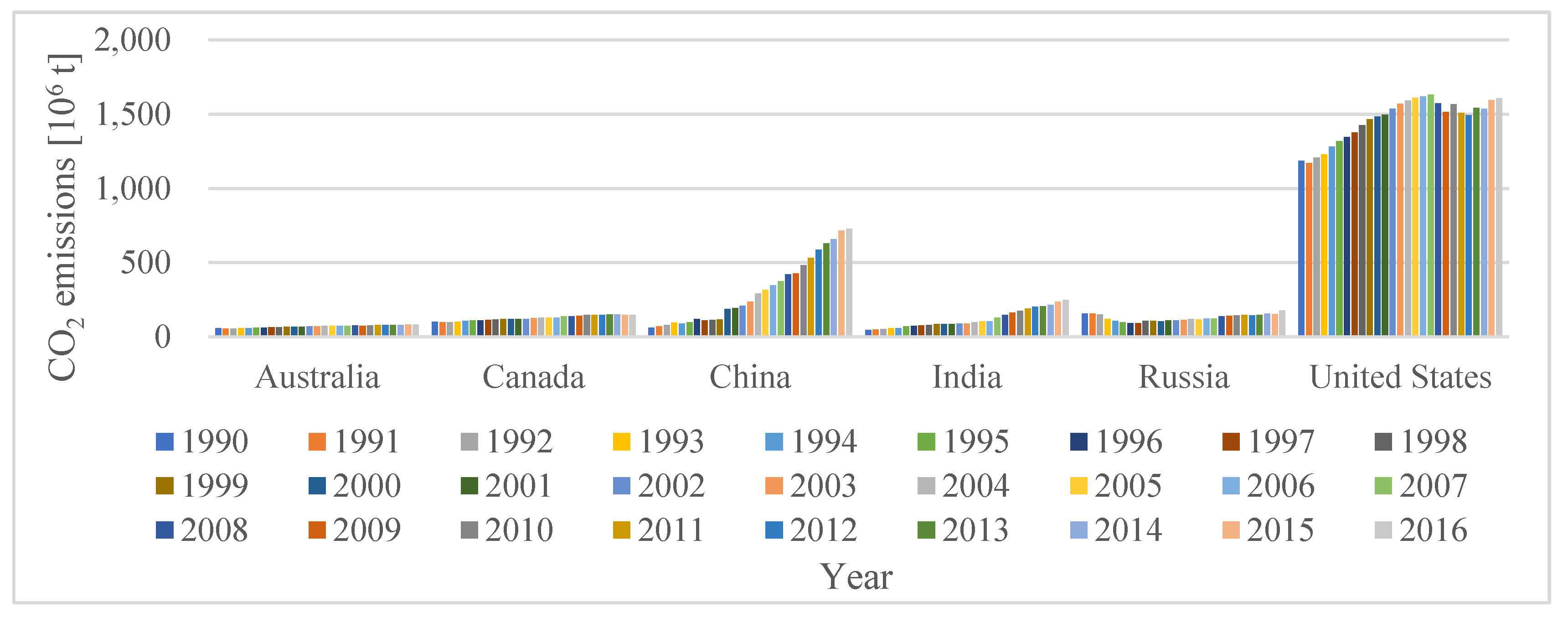
Global warming has become one of the most important challenges for human beings, and the essential cause is excess emissions of greenhouse gases such as carbon dioxide, etc. According to the statistics of International Energy Agency Data (IEA Data), the transportation industry accounted for 23.96% of the 32.5804 billion tons of global carbon dioxide emissions in 2017, making it the second largest industry of carbon emissions. Among them, carbon emissions in sub-industries of road transportation accounted for the highest proportion of the transportation industry, with more than 70%. Furthermore, according to a rough calculation in this paper, the carbon emissions of the road transportation industry in six Asia-Pacific countries (Australia, Canada, China, India, Russia, and the United States) are about 50.81% of the global total volumes of that industry. Therefore, it is of great significance to study the driving factors of carbon emissions of the road transportation industry in these six Asia-Pacific countries for controlling global carbon emissions.
Currently, relevant researches on carbon emissions of the road transportation industry mainly involve two aspects: One is the relationship between carbon emissions and economic growth, and the other is the influence factors of carbon emissions. In terms of the relationship between carbon emissions and economic growth, Grossman et al. [
1] firstly proposed an inverted U-shaped relationship between environmental quality and economic development based on Kuznets Curve (Kuznets [
2]). Panayotou [
3] called it the Environmental Kuznets Curve (EKC). Based on the EKC theory, Kwon [
4] proposed, for the first time, that whether British road transportation was fit for the turning point of EKC should be verified. Abdallah et al. [
5] verified, for the first time, that carbon emissions of road transportation in Tunisia conform to the law of EKC. With the same method, Kharbach et al. [
6], Alshehry et al. [
7], and Azlina et al. [
8], respectively, verified the applicability of EKC in the road transportation industry in the United States, Saudi Arabia, and Malaysia. However, some scholars believe that some countries cannot verify that there is an EKC relationship between environment and carbon emission (Huang [
9]).
In addition, some scholars have also verified the relationship between economy and environment through Decoupling Theory. The Organization for Economic Cooperation and Development (OECD) introduced "Decoupling Theory" and created the decoupling model. Lu [
10] used this model to verify the decoupling relationship between the economic development and carbon emissions of the road transportation industry for Taiwan, Germany, Japan, and South Korea. The study revealed that Taiwan shows a decoupling relationship, while Korea, Germany, and Japan show a relative decoupling relationship. Tapio [
11] optimized the basic decoupling model by introducing the elastic concept of economics and established the Tapio Decoupling Model to study the decoupling state of dynamic data. With this method, Sorrell et al. [
12] analyzed the energy consumption of the road freight industry for Britain from 1989 to 2004 with the decoupling analysis method. The research results showed that the United Kingdom (UK) has been more successful than most European Union (EU) countries in decoupling the environmental influences of road freight transportation from GDP. Tapio [
11] created a theoretical framework of decoupling to analyze carbon emissions of road transportation for the European Union from 1970 to 2001. The result indicated that the freight of the European Union transforms the relations from weak decoupling to expansive negative decoupling. In the 1990s, there existed a weak decoupling relation between freight transportation and carbon dioxide emissions in the UK, Sweden, and Finland, while a strong decoupling relation between road traffic volume and carbon dioxide emissions from the road transportation industry in Finland from 1990 to 2001. Kveiborg et al. [
13] combined the Divisia Index Decomposition Method and Tapio Decoupling Model to analyze the carbon emissions of road freight from 1981 to 1997. The research results presented an obvious decoupling relationship in road freight from 1989 to 1997.
The decoupling model mainly calculates the decoupling index and the decoupling factor (OECD reference) to determine whether there is decoupling relationship between the environment and the economy; however, it cannot explain the specific reasons of decoupling. Therefore, some scholars have begun to study which factors have an influence on carbon emissions. At present, the research mainly focuses on using the factor decomposition method or the econometric model to analyze the influencing factors of carbon emissions. The factor decomposition method is mainly divided into the Laspeyres Index Decomposition method and the Divisia Index Decomposition method. (The Laspeyres Index Decomposition method follows the Laspeyres price and quantity indices in economics analysis.) Hankinson et al. [
14], Reitler et al. [
15], Howarth et al. [
16], Howarth et al. [
17], Park [
18], Park et al. [
19], and Lin [
20] all used this method to analyze carbon emissions of different countries and regions. Due to the defect that the Factor-Reversal Test and the Time-Reversal Test cannot pass the tests in the Laspeyres Index method, Sobrino et al. [
21] adopted the improved Laspeyres Index method to analyze driving factors for carbon emissions of the road transportation industry in Spain from 1990 to 2010. The conclusion showed that economic growth reveals a close relationship with the rise of carbon emissions, and improved energy efficiency has been a powerful contributor to the carbon emissions decrease.
Because relatively large residual errors in the calculated results in the Divisia Index Decomposition method exist, and it cannot solve the problem of zero value, Ang et al. [
22] proposed the Logarithmic Mean Divisia Index (LMDI) in 1998. It effectively solves the above problems and acquires a wide range of applications. M’raihi et al. [
23] adopted this method to study the influencing factors of carbon emissions of the road transportation industry in Tunisia. The research results showed that economic growth is the main reason for the increase of carbon dioxide emissions. Effects of fossil fuel share, fossil fuel intensity, and road freight transport intensity are all found as secondary factors responsible for CO
2 emission changes, while Timilsina et al. [
24] considered that the economic activity effect and the transportation energy intensity effect are found to be the main driver of CO
2 emissions of road transportation in Latin American and Caribbean countries. Liu et al. [
25], Howarthetal et al. [
16], Paul et al. [
26], and Lise [
27] all used this method to analyze the relationship between energy consumption and carbon emissions.
Econometric models can effectively analyze time series data. Wei [
28] used the impulse response function and the factor decomposition method to study the carbon emissions of China’s road transportation industry. The research results showed that traffic structure and carbon emissions had long-term influences and that dynamic interactive mechanisms exited in China from 1989 to 2009. Wang et al. [
29] used a combined research model, including co-integration analysis, the error correction model, and the dynamic model, to study the influences of different factors on energy consumptions in China and OECD countries. However, the paper only showed the strong and weak relationship of each factor—it did not quantify their influence degrees. Liimatainen et al. [
30] firstly proposed the "road freight–economy" relationship analysis framework (McKinnon et al. [
31]) for McKinnon’s improvement, and introduced three indexes of CO
2 intensity, transport intensity, and energy efficiency. He used a joint analysis method for comparison to analyze carbon dioxide emissions and energy efficiencies of the road transportation industry for the four countries of Denmark, Finland, Norway, and Sweden in northern Europe in 2010. It indicated that transportation intensity and energy efficiency have significant influences on carbon dioxide emissions. Puliafito et al. [
32] calculated the carbon emissions data of Argentina’s road transportation industry from 1960 to 2010 and predicted the data from 2011 to 2050, and Monte Carlo sensitivity analysis and scenario analysis methods were applied to analyze the relations between energy demand and greenhouse gas emissions. Melo [
33] applied both the spatial and non-spatial panel data models and introduced ten influence factors, such as urbanization, vehicle ownership, and income levels, etc., to analyze the causal relationship between demand-led, as well as supply-led, factors and carbon emissions of the road transportation industry. The multi-factor and multi-angle analysis strategy provided in the paper can provide a basis for future researches on causality and influence factors. Hasan et al. [
34] used a multiple regression model to determine the main driving factors of transportation emissions of passenger vehicles in New Zealand. The results showed that there is a significant causal relationship between fuel economy and transportation emissions. The present study can provide reference values for future studies in different effect factors, and might offer further policy implications for other countries. Sundo [
35], adopting a new mathematical original-destination (O-D) approach of estimating CO
2 emissions, made a comparison among five different low-carbon scenarios. The results showed that increasing the proportion of clean energy can effectively reduce the carbon emissions of the road transportation industry.
Seen from the above references, scholars at home and abroad have conducted in-depth researches on the carbon emissions of the road transportation industry, but several problems also exist, as follows: (1) The expansion of Kaya identity is a little simpler when the factor decomposition method is used to analyze carbon emissions of transportation industry; and (2) currently, only a few scholars conduct comparative studies among countries, while other scholars take only one country as the research object, failing to fully explain the differences of carbon emissions among countries. This paper takes six Asia-Pacific countries as the research object, and expands Kaya identity by introducing transportation turnover and other indexes, so as to analyze the influence of more factors on the carbon emissions of the road transportation industry. The LMDI decomposition method is used to emphatically discuss the driving factors of carbon emissions of road transportation, and comparative studies among the six countries are conducted to analyze the influence mode and degree of various factors on carbon emissions of the road transportation industry in these six countries.
2. Research Method
2.1. Expansion of Kaya Identity
Kaya identity, firstly proposed by Japanese professor Yoichi Kaya at the seminar of Intergovernmental Panel on Climate Change (IPCC) in 1989 [
36], establishes a relationship between carbon dioxide emissions and economic, policy, as well as population factors, etc. It can decompose driving factors for carbon dioxide emissions and quantify the contribution rate of each influencing factor accurately. Its expression is as follow:
In Formula (1), C, POP, GDP, and PE respectively represent the volume of carbon dioxide emissions, the whole population of a country, gross domestic product, and total energy consumption.
Kaya identity has been widely used in the fields of energy, environment, and economy. However, due to the limited numbers of examined variables, the results obtained are basically confined to the quantitative relationships between carbon dioxide emissions and energy, economy, and population at the macro level. In recent years, when studying influencing factors for carbon emissions of road transportation, most scholars have mainly selected population size, GDP per capita, and the carbon emissions coefficient of energy [
37,
38,
39]. However, since carbon emissions are not only connected to these factors, but also relatively closely related to factors of transportation intensity and energy intensity, etc., the index of road transportation turnover is added in this paper, and the Kaya identity is extended. The expression of the expanded Kaya identity is as follows:
In Formula (2), GDP and POP have the same meaning as Formula (1); C represents total carbon emissions of a country’s road transportation industry; TRS says road transportation turnover of a country; and PE indicates energy consumptions of a country’s road transportation industry.
Formula (2) can be simplified into Formula (4) by applying Formula (3):
In Formula (4), G, R, P, S, and O respectively represent economic output, transportation intensity, energy intensity, and the carbon emissions coefficient of energy, as well as population size.
2.2. The LMDI Decomposition Method Based on Extended Kaya Identity
The factor decomposition method is a further extension of Kaya identity, mainly including the Laspeyres Index decomposition method, the Logarithmic Mean Divisia Index (LMDI) decomposition method, and the Fisher’s Ideal Index method, etc. Among them, the LMDI decomposition method, proposed by Ang. B.W. etc. in 1998, solved the problems of inherent salvage value and zero value for the index decomposition method. It witnesses an advantage of complete decomposition and the results’ uniqueness [
22,
40]. Therefore, the LMDI decomposition method has become a mainstream research tool in the field of energy and environment.
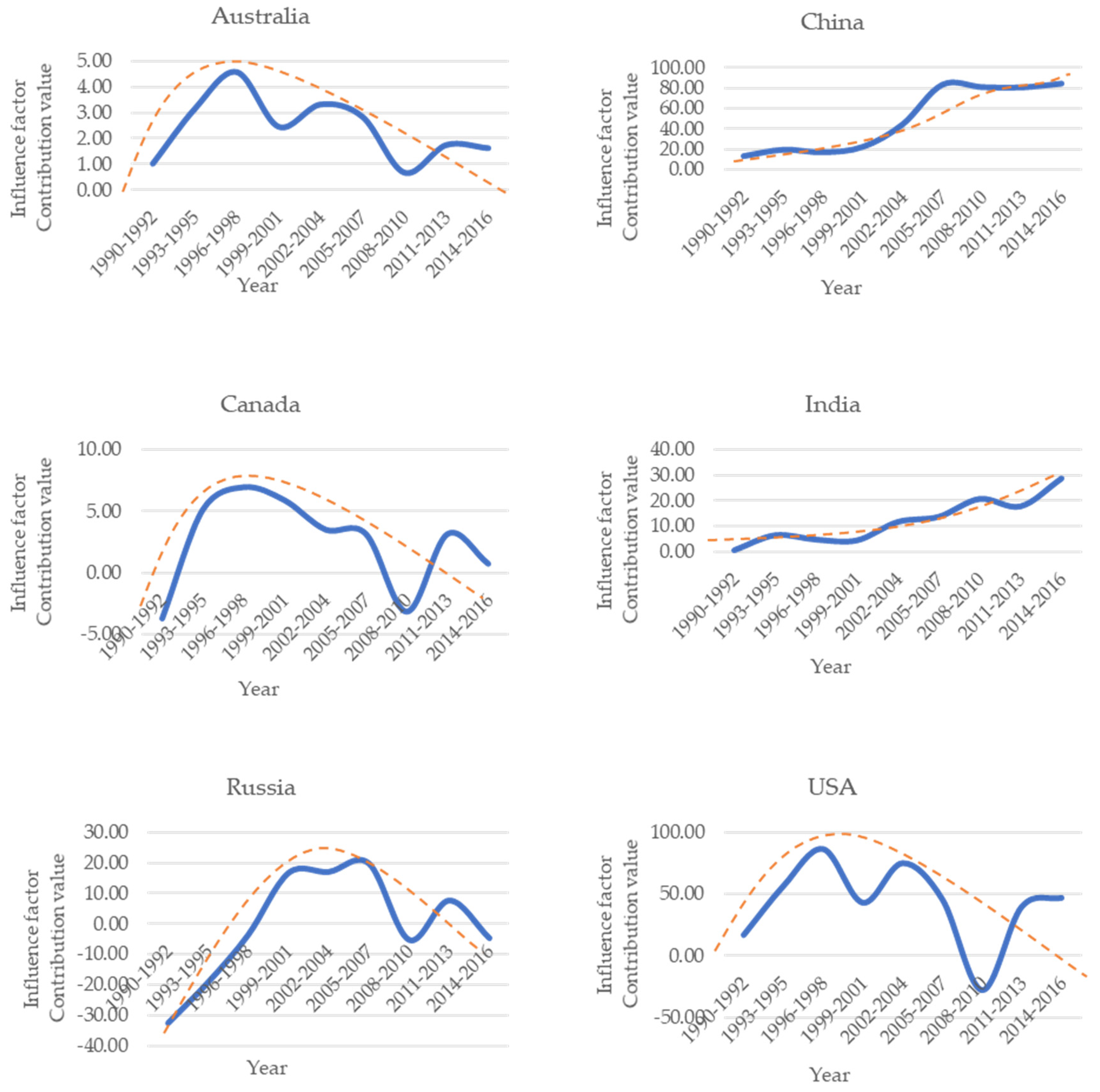
The LMDI decomposition method includes the two specific methods of additive decomposition and multiplication decomposition [
41]. Because decomposition results of the two methods can be converted to each other, and their converted results are consistent, this paper adopts the additive decomposition method to decompose the model shown in Formula (4). The specific formula is shown in Formula (5).
In Formula (5),
DG represents economic output effect,
DR represents transportation intensity effect,
DP represents energy intensity effect [
42],
DS represents carbon emissions coefficient effect of energy, and
DO represents population size effect. Hence, the formulas for calculating the effects of various factors influencing carbon emissions are shown in Formulas (6)–(10), and the detailed calculation process is included in the
Appendix A.
Here, among Formulas (6)–(10), C0 indicates the baseline year value of carbon emissions for one country’s road transportation industry; Ct represents carbon emissions of a country’s road transportation industry in year T; Gt, Rt, Pt, St, and Ot respectively show the economic output, transport intensity, energy intensity, the carbon emissions coefficient of energy, and population size in the Tth year of a country’s road transportation industry; and G0, R0, P0, S0, and O0 respectively show a baseline year’s economic output, transport intensity, energy intensity, energy coefficient of carbon emissions, and population size of a country’s road transportation industry.


