Real Time Energy Performance Control for Industrial Compressed Air Systems: Methodology and Applications ^†

Abstract

Most manufacturing and process industries require compressed air to such an extent that in Europe, for instance, about 10% of the total electrical energy consumption of industries is due to compressed air systems (CAS). However, energy efficiency in compressed air production and handling is often ignored or underestimated, mainly because of the lack of awareness about its energy consumption, caused by the absence of proper measurements on CAS in most industrial plants. Therefore, any effective energy saving intervention on generation, distribution and transformation of compressed air requires proper energy information management. In this paper we demonstrate the importance of monitoring and controlling energy performance in compressed air generation and use, to enable energy saving practices, to enhance the outcomes of energy management projects, and to obtain additional benefits for non-energy-related activities, such as operations, maintenance management and energy accounting. In particular, we propose a novel methodology based on measured data, and baseline definition through statistical modelling and control charts. The proposed methodology is tested on a real compressed air system of a pharmaceutical manufacturing plant in order to verify its effectiveness and applicability.

1. Introduction

The research presented in this paper is part of a wider research project addressed to the optimization of the energy use of compressed air systems (CAS) in manufacturing plants in the context of Italian energy intensive companies [1,2,3].

Through the information obtained by more than 15,000 energy audits and data collected through questionnaires, detailed analyses have led to the conclusion that the actual state of the CAS within the Italian industry shows great opportunities for improvement. Indeed, the analyses, on the one hand, confirmed that compressed air production accounts for quite an high portion of the overall Italian industrial sector’s electric energy consumption, and, on the other hand, revealed the widespread lack of monitoring systems to measure the energy consumption of CAS [3]. In fact, despite the importance attributed by most research and legislation to the use of reliable measures for energy efficiency and energy savings in industrial sites [4,5,6,7,8], this practice is clearly still quite far from being diffusely implemented. In addition, this is due to the limited knowledge of ensuing energy efficiency and non-energy efficiency benefits. Therefore, there are still huge opportunities for improvement for both technical and managerial aspects. In particular, the improvement of energy performance control seems to be one of the most important interventions to apply as it can provide guidance to the company in the identification of energy waste, in the of optimization of the use of energy, in the improvement of maintenance methodologies and in the assessment and verification of results in economic terms.

Moreover, the increasingly fast innovation in the fields of distributed control, smart metering and machine learning can foster the implementation of a dynamic energy control by companies [9], in an Industry 4.0 perspective. Indeed, the analysis of process data and the relationships among variables enable the acquisition of valuable insight for different applications, such as process monitoring, fault diagnosis, mode clustering, soft sensing of key variables/quality variables, etc. [10].

For example, in operations management, by comparing measured data to a highly accurate and reliable reference, it is possible to exert an efficient and more effective real time control of the performance of the system and an optimization of its operating conditions [11].

Furthermore, from a maintenance point of view, the use of advanced techniques can support the real time performance control during production, implementing faults detection [12,13,14,15], fault diagnosis [16,17] and remaining useful life estimation to support the optimization of manufacturing management and maintenance scheduling [18].

Finally, the use of real time control tools can benefit the organization also from a pure economical perspective. Modelling the energy performance of the system, in fact, allows a more accurate estimation of the energy budget, not only enabling a timely discovery of anomalous behaviors but also supporting management in the investigation of their actual causes, thus enacting an efficient control of the overall performance of the system [19].

The aim of the paper is to present a general computing approach applied to energy performance control which can also jointly support the decision-making process of three different non-energy-related activities, namely operations, maintenance and energy accounting.

The approach presented can be applied to any energy use in industry, but is here specifically tailored to CAS. The paper is structured as follows: Section 2 describes the background of the problem, discussing the different methodological approaches identified in literature to impact energy performance control and the main non-energy-related activities mentioned; Section 3 provides a description of the methodology adopted while Section 4 shows the results of the application of the proposed methodology to a real case study: the compressed air system of a pharmaceutical production plant. Finally, Section 5 ends the paper, presenting the main conclusions and implications of the study.

2. Background

In recent years, with the development of new information technologies the paradigm of the fourth technological revolution, namely Industry 4.0, has emerged. This concept is based on innovative technologies such as cyber-physical systems (CPS), the Internet of Things (IoT) and cloud computing and its aim is to achieve higher operational efficiency, productivity and automation, through a continuous integration and analysis of heterogeneous data [20,21]. Considering that some of the most prominent features of this paradigm are digitization, optimization, automation, human machine interaction (HMI), and automatic data exchange and communication, it is clear how Industry 4.0 is an industrial process of both value adding and knowledge management, supported by the use of internet technologies and advanced algorithms [21]. In this context, an important aspect of Industry 4.0 is the ability of manufacturing systems to monitor and analyze the industrial reality at different levels and with different purposes, through the use of a digital copy (“digital twin”) of the physical system, process or manufacturing phenomena studied [22,23], thus making possible the enactment of smart decisions achieved through a continuous and synchronized information flow among humans, machines, and sensors alike [24].

In particular, a growing number of publications have been dedicated in the recent years to the study of new control tools based on the use of real time data from measurement systems in the field of energy performance control as well as in the main applications mentioned before: operations, maintenance and energy accounting. While presenting a variety of methodologies and different approaches, the scientific literature in these fields tends to focus on addressing these issues separately instead of analyzing the possibility of tackling them in a joint manner.

In order to examine the implications of the methodology presented in this paper, the main aspects and opportunities arisen in the mentioned applications are here briefly described (to obtain further information about the scientific literature on these topics refer to Appendix A for a deeper analysis of the publications examined).

Regarding the energy domain, various applications can benefit from a more complex data analysis. For instance, most of the different approaches available in literature to monitor and control energy performance in industrial plants share the same main phases [25,26]: measurement plan and data collection, baseline definition, implementation of control over time through comparison between the baseline, and monitored energy consumption. However, various techniques might be used to characterize the baseline energy performance of the system, depending on its complexity and on the availability and quality of data (e.g., air compressors, boilers, pumps, buildings, etc.) [27,28,29,30,31,32,33]. Often, for this purpose, statistical regression is used, and more recently—machine learning methodologies, such as artificial neural networks or support vector regression; all of which have been tested. The most common approach is to evaluate the residual between actual energy consumption and the prediction obtained from the baseline model. In order to help the evaluation of the residuals’ significance, control charts, such as EWMA (exponentially weighted moving average), CuSum (cumulative sum) or Shewhart charts are used [27,28,30].

Other important applications developed due to the availability of real time data are the prediction of energy consumption, especially critical for building management [34,35,36,37,38,39,40,41] and electrical load management [42,43,44,45,46,47,48,49,50,51,52,53,54], and the forecast of energy production by renewable energy systems (mostly used for wind turbines and photovoltaic panels) [55,56,57,58,59].

Process control and performance monitoring are other fields interested in the innovation brought by data analytics tools. For instance, some data-driven models are used to give online estimation of key variables that, due to technical or economic limitations, would be too difficult to measure otherwise [60,61], while other models are used to perform process monitoring in order to detect anomalies [62].

In regards to maintenance, instead, depending on the specific application, different goals can be achieved: condition-monitoring, fault detection, diagnosis and prognostics. The more complex the objective, the more complex the model and the data used to achieve it. Therefore, while condition monitoring [63,64,65], fault detection [66,67] and diagnosis [12,13,14,68] may be achieved even with statistical models, prognostics models are usually developed through machine learning techniques [17,18,69,70,71,72,73,74,75]. Both supervised and unsupervised approaches are used in fault detection, diagnosis and prognosis (e.g., artificial neural networks, decision trees, ARMA (autoregressive moving average) or logistic regression models, etc.) [73].

Finally, the scientific literature related to energy accounting is still limited. In fact, while energy efficiency is finally regarded with attention in the industrial context, the cost of energy is still not widely analyzed. Some papers propose methodologies to predict the energy budget using variables of influence to estimate the energy consumption through statistical modelling [76,77]. Moreover, the differences between budget and actual costs can be analyzed through indicators that distinguish the effect of different specific causes (e.g., different prices, production volumes, on-site generation system efficiency, etc.) [76,78,79].

3. Methodology

The methodology described herein defines a series of steps for a real time energy performance control organized in a replicable process in order to facilitate their implementation in different industrial contexts.

The methodology was developed to be as widely applicable as possible (at least to a wide range of different industrial auxiliary systems) but is here particularly referred to CAS. It is fundamental to highlight that the paper focuses on energy performance rather than energy consumption. This entails a combined measure and integrates analysis of CAS’ energy consumption and compressed air production which has the potential to provide much more information to the final user of the control system.

Moreover, one main innovative aspect of the proposed methodology is its capability of impacting, in a jointly manner, three different non-energy-related activities (operations, maintenance and accounting): (i) the definition of the best operating conditions of a system from an energy efficiency perspective; (ii) the identification of changes to energy consumption patterns or degradation of energy performances linked to sporadic faults or events and (iii) the achievement of a deeper understanding of the energy behavior of the overall system aimed at an improved energy accounting.

The methodology is developed following an empirical approach, on the basis of needs and requirements identified through a close collaboration with industrial practitioners involved in the case study and afferent to the different functions, such as energy, operations and maintenance management. Some of the tools integrated in the methodology adopt features from similar non-energy-related tools already in use, such as quality and process control tools as well as project management tools [9,10,27,28,76,77], in order to overcome implementation barriers mainly related to usability and resistance to change. As a result, people involved in the case study are able to work with familiar tools, even though based on new data analysis and real time control concepts and applied to the energy management context.

The rest of this section is organized as follows: the first subsection illustrates the overall methodology for real time energy performance control, while following subsections will be dedicated to each application.

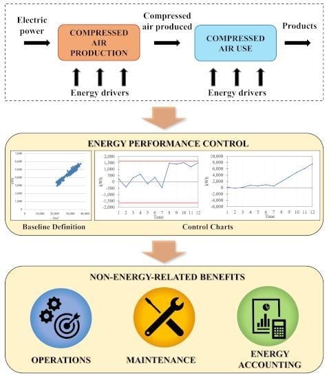
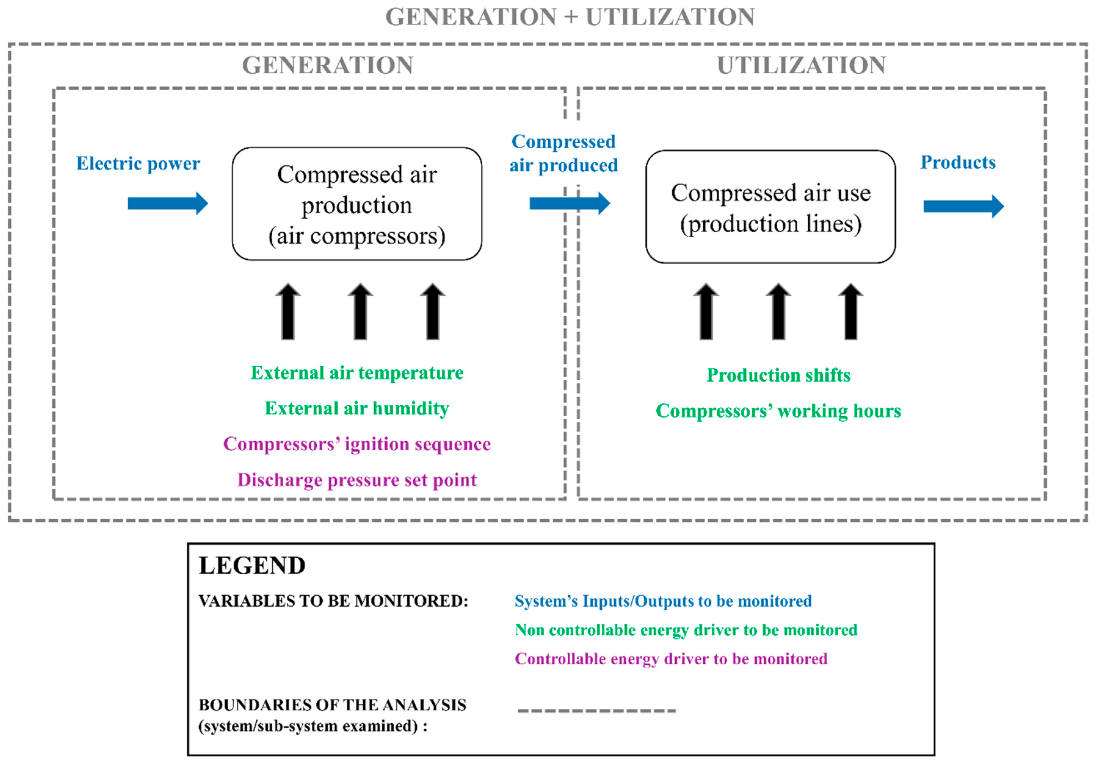
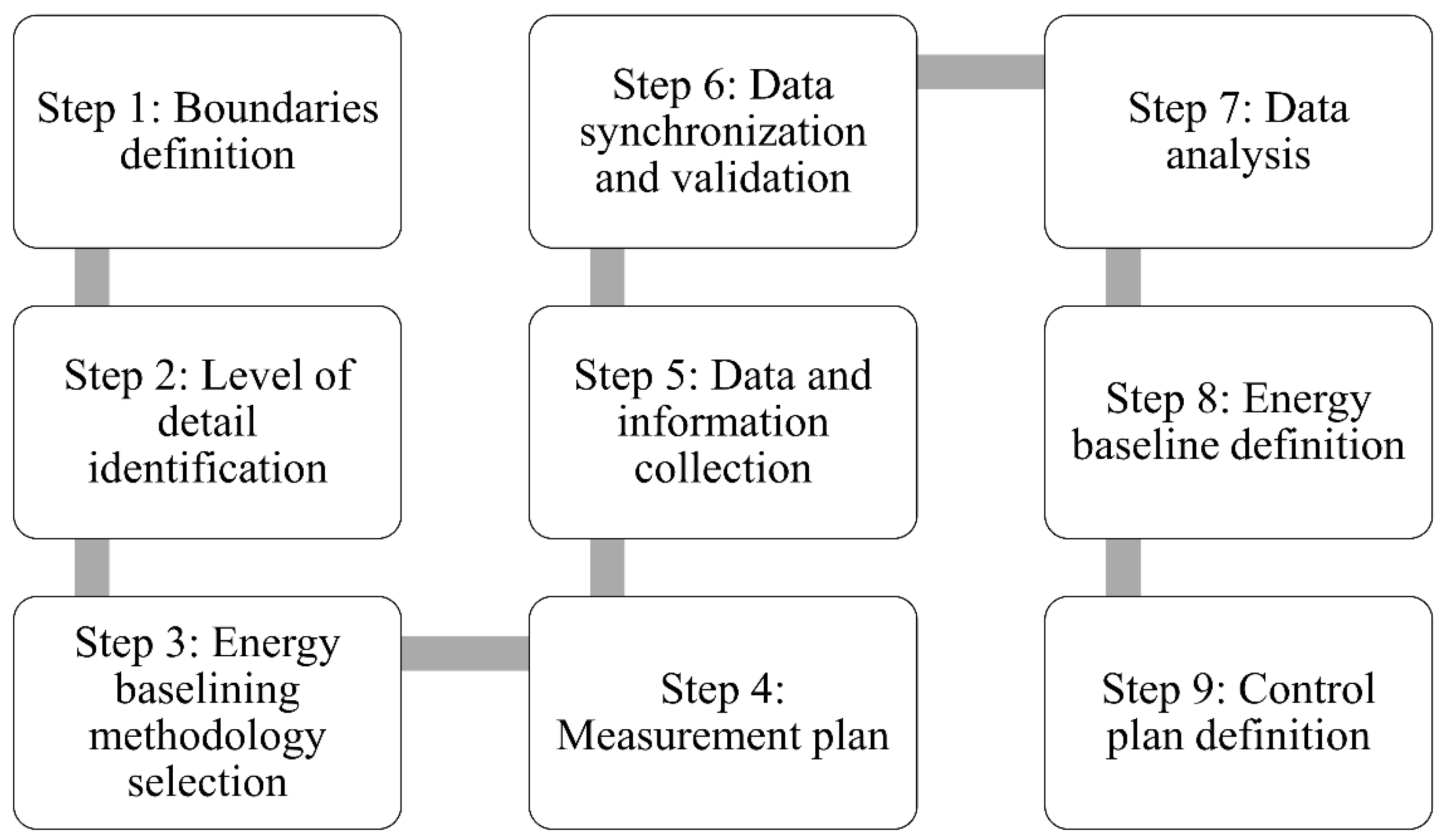
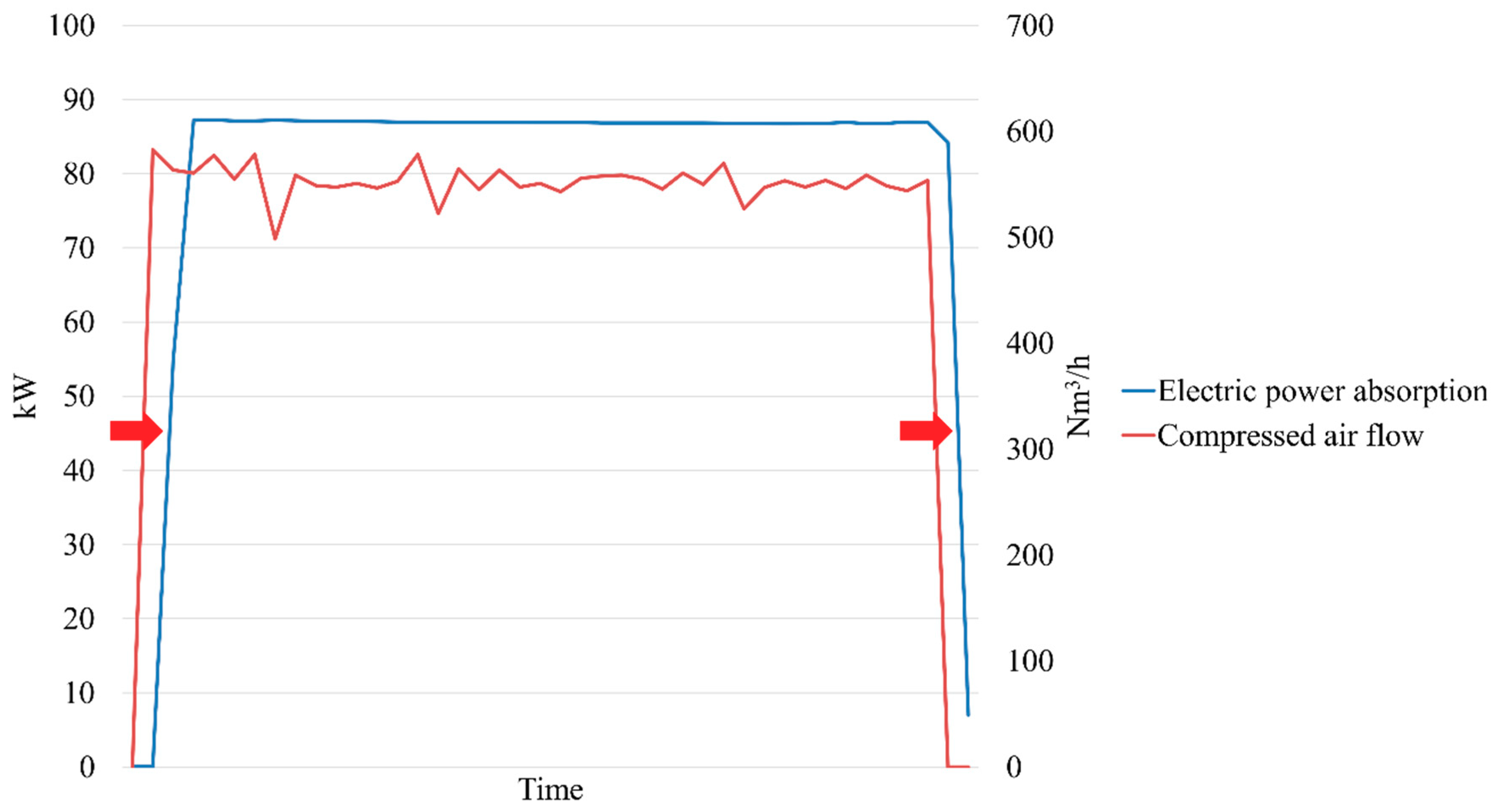
3.1. Methodology for Real Time Energy Performance Control

The methodology is built on statistical tools for energy measurement and verification and energy monitoring and targeting [6,19,28], which were then customized for real time energy performance control (and auxiliary industrial systems, with particular focus on CAS) in order to draw a complete picture of the system’s energy behavior, and therefore, create a reliable baseline.

Figure 1 gives a schematic representation of the most common variables to be monitored for CAS and the different possible boundaries of the analysis. Compressed air generation and utilization are represented together with their main inputs/outputs and all the main variables that are capable to influence the energy performance of the system, also called “energy drivers” [19]. Energy drivers are divided into two categories, i.e., controllable and non-controllable. Controllable energy drivers can be modified by the companies and set by operators, while non-controllable energy drivers cannot be modified (either because out of company’s control, such as weather conditions, or because the company is not willing to change them to improve energy efficiency, such as production rates and working hours).

The methodology, represented in Figure 2, is made up of nine steps, briefly illustrated in the following.

Step 1 is the definition of the boundaries of the analysis. In this preliminary step, it is important to identify the main typologies of energy carriers (defined by the International Organization for Standardization as “substance or medium that can transport energy” [80]) and the transformations that they underwent. In particular, when examining a specific energy carrier, it is useful to distinguish between its generation and its utilization in order to be able to address the needs of different users in term of control (e.g., top management, operations managers, utilities managers, maintenance operators, etc.). For example, considering CAS, it is necessary to understand whether the analysis should focus on compressed air production (the generation of compressed air by air compressors using electricity), utilization (the use of compressed air by production equipment), or both.

Once boundaries are defined, it is necessary to identify the level of detail of the analysis (Step 2) in terms of space and time, determining, for example, whether it is more convenient to take into account the whole plant, a single department or just one production line or machine, and, moreover, defining the most suitable frequency at which analyze energy data. This second choice is made considering the thermodynamics of the process/system, the purpose of the control and the type of users of the implemented control system: a low frequency (e.g., from a few hours to a few days) is generally used for strategic control purposes whereas a higher frequency (e.g., from 10 to 30 min) is more suitable for operational control.

The third step is the energy baseline method definition. Among the several methods available to analyze data and to build the energy baseline, we chose statistical regression [25,27,81,82] as the most effective to organize the data collection accordingly. However, physical models, artificial neural networks or even machine learning techniques [15,28] are employable. First of all, it is important to highlight that the choice of the method mainly depends on the following factors: (i) available resources for the control system ramp-up; (ii) available resources for the control system maintenance; (iii) boundaries and chosen level of detail (i.e. the need to analyze several assets at the same time); and (iv) the need to keep a deep understanding of the thermodynamics controlling the process (i.e. highly automated tools generally allow a lower understanding, as they rely on “black box” methods).

As energy consumption is often dependent on several variables, the characterization of the energy behavior requires the collection of different types of information: consumption data, production data, environmental data, technical (users) and operational data [26]. Therefore, a measurement plan is implemented (Step 4) with the aim to perform an appropriate data collection for all the variables (inputs, outputs, energy drivers) that need to be monitored, paying special attention at their coherence (same period of time and frequency) and at identifying the appropriate measuring systems and the additional information that needs to be collected (e.g., maintenance schedules, production data). The amount of data and information collected and the consequent resources committed in this phase are defined accordingly to the entity of the potential saving achievable with real time control, while also establishing a duration of the data collection phase such as to guarantee a correct representation of all possible working conditions.

In the following phase (Step 5), the measurement plan illustrated above is implemented and data collection activities are performed.

Step 6 aims to check and solve any synchronization issues and to implement manual or automatic data handling, depending on the amount and quality of the collected data. Inaccuracies introduced by the measuring system are also corrected in this moment. Moreover, it is necessary to perform a first data validation in order to avoid poor/low quality data and meters’ faults.

Afterwards, on the basis of the choice made in the third step, a model that characterizes the energy behavior of a system from a set of collected data is developed in Step 7 in order to enable the investigation of intrinsic and external causes of energy performance variability.

The first statistical tool is the correlation analysis of the previously collected energy drivers and energy consumption data to define the dependence of the energy behavior of the system on identified energy drivers, thus allowing preliminary qualitative considerations. Moreover, in order to get more quantitative information, it is possible to perform regression analyses, using the coefficient of determination (i.e., R²) and the related probability (i.e., P_value) [81,83] to analyze the strength of the correlation and select the energy drivers on the basis of their actual influence.

Once the first model that included all the available data has been created, a validation and a first analysis of the overall performance of the system is carried out. Among the control charts used in quality control [83], two of them are particularly suitable for this kind of analysis.

First of all, let E_ac(t) be the actual energy consumption of the system at time t and E_pd(t) be the energy consumption predicted through the use of the baseline model for the same time t. The difference between these two values is the energy performance deviation, defined as ΔE(t) and calculated as follows:

$$\mathsf{\Delta }\mathrm{E}\left(\mathrm{t}\right)={\mathrm{E}}_{\mathrm{ac}}\left(\mathrm{t}\right)-{\mathrm{E}}_{\mathrm{pd}}\left(\mathrm{t}\right)$$

(1)

The evolution over time of this parameter (ΔE(t)) can be observed in a first control chart—the control chart for energy performance deviations. Every point in the chart represented the energy performance deviation at a specific time (Figure 3a). Two lines, the upper and lower control limits, are added to the chart to support the analysis of the energy behavior of the system. These two control limits (UCL—upper control limit; LCL—lower control limit) are evaluated starting from σ, the standard deviation of the statistical distribution of ΔE(t), as follows:

$$\mathrm{UCL}=+\mathrm{k}\times \mathsf{\sigma }$$

(2)

$$\mathrm{LCL}=-\mathrm{k}\times \mathsf{\sigma }$$

(3)

The coefficient k used in the equations is conventionally set to 3, but as the control chart’s sensitivity is established by the width of its control limits, the coefficient k may also be set to a lower value in order to enact a stricter control. When the system examined shows an energy consumption behavior compliant with the baseline model, the energy performance deviations on the chart displays a normal statistical distribution with mean equal to zero, on the contrary, the presence of nonrandom patterns (e.g., points outside the control limits, mixtures or shits of the average) are signals of non-conformity with the baseline model and therefore of anomalous behavior.

Moreover, a second control chart, the cumulative sums chart, or CuSum, is used to deepen the analysis of the energy behavior of the system. Every point in the CuSum chart shows the value over time of the cumulative sum of energy performance deviations, defined as $\mathsf{\Delta }\mathrm{EC}\left(\mathrm{t}\right)$ and is calculated as follows:

$$\mathsf{\Delta }\mathrm{EC}\left(\mathrm{t}\right)={{\displaystyle \sum }}_{t=0}^t\mathsf{\Delta }\mathrm{E}\left(\mathrm{t}\right)$$

(4)

This type of control chart is useful because it highlights trends in energy performance behavior (Figure 3b). Indeed, a change in the slope of the CuSum represents a variation in the energy behavior of the system.

The joint examination of these two control charts supports the identification of different energy behaviors within the observed period or sub-periods and the identification of an accurate baseline model (i.e., the energy behavior that is taken as a reference to compare future performances).

The baseline model can be identified (Step 8) in the following three ways [19], depending on the choice of the set of data:

• considering the most recent available one; this choice is the best one when changes to technical, technological or structural configurations of the analyzed center occurred;
• considering the data set that showed the best energy performance; this choice is usually considered with a view to continuous improvement because it implies a more challenging outcome in terms of energy objectives;
• considering the data set that showed the most constant and stable energy behavior; this choice is generally made when none of the two previous options is applicable.

It is worth noting that, in any case, the sub-period chosen to create the baseline model should allow an accurate statistical data analysis, and therefore, it should be sufficiently long to include enough data. In some cases, where the cyclic nature of the energy consumption is evident (e.g., when the external temperature has a strong influence on the energy efficiency of the system), it might be appropriate to build different energy baselines for different time periods or conditions, defining when it is necessary to switch from one baseline model to another. In this phase, it is also possible to validate the baseline model by using all the available additional information, mainly related (but not limited to), operations and maintenance. This allows matching most of the variations from the baseline energy behavior occurring during the observed time period with actual events happened to the system (e.g., periodic maintenance interventions, shutdowns, etc.) and therefore, verifies the effectiveness of the model itself and of the control charts. This specific activity is usually time and resource consuming, as it is necessary to collect more information and to interview operators and maintenance personnel.

In the final step (Step 9), it is possible to use the baseline model to implement a continuous control over time. Real time data for both energy consumption and energy drivers are acquired by metering systems and their differences (i.e., ΔE(t)) are evaluated at the chosen frequency (or at different/multiple frequencies, depending on users’ needs) and represented on the control charts to highlight the presence of possible anomalies, enabling a real time control by the users. Moreover, the setting of control limits and other alarm conditions can automatize the generation of alerts to foster a timely response.

3.2. Definition of the Best Operating Conditions of a System From an Energy Efficiency Perspective

The methodology previously illustrated (Steps 1–7) is implemented in order to evaluate different operating conditions for the system and identify the best option from an energy efficiency perspective. In fact, it is sufficient to include in the data collection period, different sub-periods where operating conditions are different (e.g., different time sets, different pressure sets, different starting sequence, etc.). In many cases this happens automatically by considering a long data collection period or is achieved by switching such conditions on purpose during the data collection process.

Since different energy behaviors can be distinguished through the analysis of control charts (Step 7) and energy performance variations due to energy drivers’ variability are already within the model, only the energy consumption variability due to the different operating conditions is made visible on the control charts. The evaluation of different operating conditions is therefore, made more accurate and effective. Moreover, the whole of Step 7 can also be iterated in different moments if a new evaluation is required during the control phase (e.g., when a new operating condition is introduced).

3.3. Identification of Changes to Energy Consumption Patterns or Degradation of Energy Performances Often Linked to Sporadic Faults or Events

The methodology previously illustrated (Steps 1–9) can also be implemented in order to identify a system’s malfunctioning. The control charts can, in fact, be used over time to identify variations in energy behavior which can in turn be related to fault events through further investigations (in a similar way as the one described in Step 8).

In addition, it is possible to set up a registry (similar to fault registries already in use in industry for maintenance management purposes [84]) where all anomalies identified in the charts are collected together with relevant information such as time and entity of the deviation, values of all energy drivers, operating conditions, and causes of the anomaly. This kind of registry enables the analysis and classification of anomalies and allows identifying recurrences, patterns and similarities in the control charts, in order to promote the association of the most likely causes for each new anomaly in a quick and automatic way on the basis of past events (e.g., progressive obstruction of air compressors’ filters resulted in a typical slope of the CuSum chart).

The creation of the registry and the analysis of past anomalies also increases the efficiency of the control system, as it is possible to identify anomalies related to inaccuracies of the control system itself rather than to actual issues of the observed physical system. Therefore it prevents false alarms (such as a meter’s fault, missing data or a specific condition where the statistical model loses accuracy), thus enabling the user of the system to immediately activate the functions/units in the company that are most likely to be able to solve the issue. This registry can be compiled manually or automatically, implementing pattern recognition techniques [85], depending on system’s characteristics and available resources.

3.4. Improved Energy Accounting

Energy accounting in industrial companies can be ineffective, as discerning between energy consumption variations to be expected (e.g., due to production volume variations) and actual anomalies (e.g., faults) is difficult without using an appropriate energy baseline. With the proposed methodology (Steps 1–8), once a proper energy baseline is created, it is possible to setup the earned value, a tool widely diffused for accounting in project management [86] whose application to energy management has already proved to be effective [76,87].

Such a tool requires a distinction between the actual values of energy consumption (measured, indicated in the followings as C_A) and the predicted ones (calculated using the baseline model, and indicated in the followings as C_P), calculated for budgeting purposes. In this case, the C_P values are calculated months before the energy is actually consumed by inputting the predicted values of the energy drivers into the baseline model. This means that the difference between C_A and C_P includes both energy efficiency and energy drivers’ variations, and therefore it is not possible to distinguish actual inefficiencies from physiological variability. As a consequence, it is necessary to introduce another type of calculated energy consumption, named “flexible consumption” (C_F), which is calculated through the baseline model, using the actual values of the energy drivers as inputs. At this point, the difference between C_F and C_P represents the physiological variability of energy consumption (due to energy drivers’ variations and here indicated as ΔP), while the difference between C_A and C_F represents the energy loss related to inefficiencies of the system (here indicated as ΔI).

$$\mathsf{\Delta }\mathrm{P}={\mathrm{C}}_{\mathrm{F}}-{\mathrm{C}}_{\mathrm{P}}$$

(5)

$$\mathsf{\Delta }\mathrm{I}={\mathrm{C}}_{\mathrm{A}}-{\mathrm{C}}_{\mathrm{F}}$$

(6)

Since this application aimed at facilitating energy accounting, it is necessary to shift from energy consumption to energy cost, multiplying C_A by a standard energy unit cost. Such a unit cost comprises energy purchasing and on-site energy production costs and allocates them to a single energy unit (e.g., €/kWh). Again, since the budget is usually calculated months before the energy is actually consumed, in order to take into account the possibility of differences in the energy price, it is necessary to distinguish between the predicted standard energy unit cost (indicated as c_P), which is calculated in advance, and the actual standard energy unit cost (indicated as c_A in the following), resulting from electricity and fuels bills. The energy budget variance due to differences in energy prices (Δp) is, therefore, calculated as follows:

$$\mathsf{\Delta }\mathrm{p}=\left({\mathrm{C}}_{\mathrm{A}}\times {\mathrm{c}}_{\mathrm{A}}\right)-\left({\mathrm{C}}_{\mathrm{A}}\times {\mathrm{c}}_{\mathrm{P}}\right)$$

(7)

This analysis is usually performed at time steps at which the energy budget is calculated, at least on a monthly basis. However, it could be in principle applied to any time step at which the energy baseline is calculated.

4. Case Study

The proposed methodology was applied to monitor and control the energy performance of the compressed air system of a pharmaceutical production plant located in central Italy, in order to get a first validation and to verify its applicability to the three non-energy-related activities illustrated in the previous section.

For what concerns Step 1, the company decided to focus on the compressed air production phase in order to identify additional improvement opportunities and to verify its correct operation and energy behavior (data were already available but had never been actually analyzed before). The plant was equipped with five screw compressors divided into two groups installed in separate sections of the industrial plant. We referred to these sections as room “A”, hosting two of the five compressors, and room “B”, with the other three compressors.

The maximum compressed air production was higher than the maximum compressed air demand, and usually only two or three compressors work simultaneously. Only Compressor 5, located in room “B” had a variable speed drive installed, and it served as “master” (continuously functioning), while the others worked as load/unload and served as “slaves”. A central control system regulated the compressors in accordance with compressed air demand. Some general information on the compressors (nominal and stand-by nominal power) is reported in Figure 4. Data related to energy consumption and compressed air production, as well as compressed air pressure, external air temperature and humidity were available with a 15 min frequency (i.e., already collected, recorded and stored in the company’s servers), while the number of hours worked by each compressor was available weekly (cumulated).

The level of detail of the analysis (Step 2) was defined by the company on the basis of three main observations: (i) the energy manager wanted to properly exploit existing data, which was considered to be relevant but had never been used to retrieve information on the system’s performances, (ii) there was very little budget at that time to buy new meters, and the energy manager wanted to use results from a first system’s analysis to justify additional budget allocation for new meters and (iii) for a first analysis of the system, the energy manager aimed at having general information on the whole system’s performances rather than on single compressors.

All measured parameters (i.e., compressed air production, compressed air pressure, external air temperature and humidity, hours worked by each compressor) were considered as potential energy drivers and the first data analysis was conducted taking all of them into account, apart from the amount of worked hours, as it was available at a lower frequency. In fact, for this first analysis, aimed at defining the energy drivers as well as the energy behavior of the system, a daily frequency was considered to be the most appropriate, and a data collection period of one year was adopted.

Considering the amount of data to be processed and the company’s needs, the baselining method selected was the statistical analysis (Step 3). It is important to point out that, although in this case a statistical regression was able to provide an appropriate baseline model, this method might not always represent the best choice. Indeed, for every specific case, the right baseline method should be identified taking into account the complexity and the dynamic of the system as well as the amount of data available.

Since there were constraints in terms of budget, and the data available were more than sufficient to conduct the analysis at the defined level of detail, the measurement plan and data collection (Steps 4–5) were performed considering the already available data. A synthesis of the measurement plan is given in the

Table 1. Measurement plan.

	MEASURED DATA
	Label and Unit	Frequency	Collection Period	Meter/Collection Method
Inputs /Outputs	Electric absorption compressor 1 [kW]	15 min	Last solar year (April to April)	Schneider PM9C energy meter; data on company’s online server
	Electric absorption compressor 2 [kW]	15 min	Last solar year (April to April)	Schneider PM9C energy meter; data on company’s online server
	Electric absorption room B [kW]	15 min	Last solar year (April to April)	Schneider PM9C energy meter; data on company’s online server
	Compressed air flow room A [Nm3/h]	15 min	Last solar year (April to April)	Emerson Rosemount™ 485 Annubar™ (averaging Pitot tube); data on company’s online server
	Compressed air flow room B [Nm3/h]	15 min	Last solar year (April to April)	Rosemount™ 485 Annubar™ (averaging Pitot tube); data on company’s online server
Energy Drivers	External temperature [°C]	15 min	Last solar year (April to April)	Data transmitted by closest weather station
	External humidity [%]	15 min	Last solar year (April to April)	Data transmitted by closest weather station
	Pressure set point [bar]	15 min	Last solar year (April to April)	Juno Midas pressure transmitter; data on company’s online server
	Compressors’ working hours	Weekly	Last solar year (April to April)	Measure collected by operators on each compressor’s screen and recorded on a shared spreadsheet

.

An accurate data synchronization and validation (Step 6) was performed in order to correctly aggregate data to the chosen frequency (from 15 min to one day), the level of detail (summing up data related to different compressors) and to avoid meters’ inaccuracies in affecting the data analysis. First of all, some flaws were identified and corrected by observing and comparing measured data: a 15 minute delay was observed between electricity consumption and compressed air production (as shown in Figure 5) and bad compressed air flow meters’ calibration (meters measuring compressed air flow while compressors were off, as shown in Figure 6).

In addition, the data collection period was reduced from one year to seven months due to frequent failures and maintenance interventions occurred to the compressed air meters during the remaining five months (see Figure 6).

The first data analysis (Step 7) was conducted through correlation and regression, considering the system’s energy consumption and the identified energy drivers in the data collection period. As a result, the only parameter showing a satisfying correlation with the energy consumption of the compressors and no multicollinearity with the other parameters, was the amount of compressed air produced, as reported in

Table 2. Results of the regression analysis.

Regression Analysis Results Considering All Parameters		Regression Analysis Results Considering Only Compressed Air Production
Coefficient of determination (R2)	0.96	Coefficient of determination R2	0.94
P_value	9.45 × 10−137	P_value	1.69 × 10−125
P_value intercept	0.76	P_value intercept	0.34
P_value compressed air production	8.32 × 10−119
P_value external temperature	2.06 × 10−17
P_value external humidity	0.01
P_value pressure	0.84

. The results of the multicollinearity analysis are represented in the form of a correlation matrix with a color scale in Figure 7.

The pressure referred to in the correlation analysis was the discharge pressure of the compressed air generation system and since it was considered a set point, the system was equipped with an advanced control in order to minimize its fluctuations. The pressure at which the compressed air was produced was around 6.5 bar, normally oscillating between 6.4 and 6.6 bar, during weekdays, while it was reduced to 6.2 bar (with a variation range between 6.1 and 6.3 bar) on weekends. These limited variations explained the limited effect on the regression model of this variable, usually quite critical for this kind of analysis. Moreover, the ambient conditions, were also examined in terms of external temperature and external humidity for a whole year in order to guarantee the analysis of the complete range of conditions possible, affecting poorly the regression model.

The resulting mathematical model of the system’s energy consumption was as follows:

$$\mathrm{Energy}\mathrm{consumption}\left[\mathrm{kWh}\right]=0.1575\times \mathrm{Compressed}\mathrm{air}\mathrm{produced}\left[{\mathrm{Nm}}^3\right]–80.02$$

(8)

This is also represented in the scatterplot in Figure 8.

The CuSum and the control chart for the energy performance deviations for the data collection period (Step 8) are given in Figure 9 and their joint observation shows the presence of four energy behaviors, highlighted using different colors. Indeed, the CuSum in Figure 9a shows four different trends clearly distinguishable and the control chart for the energy performance deviations in Figure 9b displays four different distributions with a different mean.

The causes of these different behaviors were further investigated, mainly through the observation of daily consumption data over time and interviews to operators, and they were finally identified to be the following:

• Red period (“A”): Compressor 2 presented a higher specific consumption until around day 325 when a maintenance intervention solved the problem;
• Green period (“B”): a change to the activation sequence caused Compressor 3 to work mainly with Compressor 5, whereas the others were usually kept turned off;
• Orange period (“C”): Compressor 1 presented an evident malfunctioning, remaining stuck in stand-by for three whole consecutive days;
• Blue period (“D”): another change to the activation sequence caused Compressor 4 to work mainly with Compressor 5, whereas the others were usually kept turned off.

Thus, through the analyses, two different maintenance-related events were highlighted and it was revealed that the energy behavior of the system was strongly related to the set of operating compressors and therefore to the compressors’ activation sequence (also confirmed by further analyses on the amount of hours worked by each compressor).

The baseline was then created using data from the green period (“B”) which was the one showing the best energy performance. The data analysis (Step 7) was then repeated in order to develop the mathematical model for the baseline. Results are not given in full here for sake of brevity.

4.1. Definition of the Best Operating Conditions of a System from an Energy Efficiency Perspective

An optimal starting sequence was, therefore, identified (the one corresponding to the green period B in Figure 9) and uploaded into the central control system. Some trials were performed involving the operators working on the plant’s technical systems and production lines and maintenance personnel, in order to make sure that the new starting sequence proposed suited the company’s needs best.

Control charts, built using the selected baseline as a reference (Step 9), were then used for continuous monitoring and control. In this case, the company decided to build a control system with a slightly higher level of detail compared to the previous analysis. In particular, three CuSums were employed: one for the whole compressed air generation system, one for Room “A” and one for Room “B”, in order to allow an easier and faster troubleshooting. Accordingly, two control charts for the energy performance deviations were also created: one for Room “A” and one for Room “B”. The frequency used for the analysis also increased, aggregating data every four hours. This allowed management to use relevant information coming from control charts observation for defining operations and maintenance short-term strategies. It is worthy to note that some iterations of Steps 7 and 8 were needed in order to create different baselines for the two rooms (again, full details are not given here for sake of brevity). The energy performance control results (control charts plots) for about two months are given in Figure 10, which clearly show a stable system’s behavior apart from some isolated issues mainly related to metering system’s faults.

4.2. Identification of Changes to Energy Consumption Patterns or Degradation of Energy Performances Often Linked to Sporadic Faults or Events

Once the control system was finally up and running, the operations and maintenance team gathered in order to discuss each single event highlighted by the control charts and to start setting the anomalies registry up. Taking all occurred events into account, an initial classification was created by defining a severity scale (from 1 to 4) defined according to the deviation’s entity. Then, most likely causes for each category were listed in order to facilitate troubleshooting activities. This initial version of the anomalies’ classification is given in Figure 11. The troubleshooting system has not been automated yet, as data from a longer control period were needed in order to perform more relevant analyses.

4.3. Improved Energy Accounting

The proposed methodology was also applied to energy accounting, in order to obtain more accurate predictions of the energy budget related to the use of compressed air in the production plant (intended as the total cost of electricity necessary to the generation of compressed air). Budgeting activities were performed for both compressed air generation and use, thus additional baselines models for the two production departments using compressed air were created following the same methodology. A new baseline was also defined for the compressed air generation system, as in this case, a monthly frequency was chosen for data analysis. Figure 12 gives a schematic representation of the energy accounting methodology proposed to predict the energy budget related to the compressed air used in the production plant, highlighting the boundaries of cost/responsibility centers (Dept. 1, Dept. 2, generation system, energy purchasing office).

From the monthly volume of production established for the following months, through the use of two different statistical models, the expected compressed air consumption to be used by the two departments in the plant was calculated. Then, using the sum of the expected compressed air consumption values for the two production departments as a driver for another statistical model, the electricity consumption of the compressed air generation system was also determined. The energy budget was then calculated as the product between the estimated electricity consumption and the predicted standard unit cost of electricity. Finally, the predicted standard unit cost of compressed air produced was calculated by dividing the budget by the total amount of compressed air consumption predicted.

Table 3. Estimated compressed air budget for the considered trimester.

ESTIMATED BUDGET
Month		1	2	3
Production Dept. 1	Units	4,047,800	3,757,201	3,294,456
Production Dept. 2	Units	5,475,148	4,427,156	5,889,159
Compressed air consumption Dept. 1	Nm3	12,805,432	11,219,241	8,693,420
Compressed air consumption Dept. 2	Nm3	15,916,589	12,785,528	17,153,518
Electricity consumption of the generation phase	kWh	4,448,464	3,664,935	3,970,917
Standard unit cost of electricity	€/kWh	0.158	0.158	0.158
Standard unit cost of compressed air	€/m3	0.024	0.024	0.024
Estimated budget Dept. 1	€	313,362	270,638	211,023
Estimated budget Dept. 2	€	389,495	308,421	416,382
Estimated budget for the generation phase	€	702,857	579,060	627,405

gives all details related to the estimated energy budget of the compressed air system for three months.

At the end of the trimester, once the actual flows of the energy consumed and actual standard unit costs were known, it was possible to analyze the variations occurred between predicted values and the actual ones to economically assess the performance of the plant in regards to production and use of compressed air (see

Table 4. Actual compressed air budget for the considered trimester.

ACTUAL BUDGET
Month		1	2	3
Production Dept. 1	Units	3,679,818	3,415,637	3,361,690
Production Dept. 2	Units	6,016,646	4,865,007	6,009,346
Compressed air consumption Dept. 1	Nm3	10,531,292	8,339,483	9,268,500
Compressed air consumption Dept. 2	Nm3	17,317,964	14,076,891	17,130,719
Electricity consumption of the generation phase	kWh	4,114,206	342,4346	4,220,230
Standard unit cost of electricity	€/kWh	0.159	0.159	0.159
Standard unit cost of compressed air	€/m3	0.023	0.024	0.025
Estimated budget Dept. 1	€	247,372	202,558	235,587
Estimated budget Dept. 2	€	406,786	341,913	435,429
Estimated budget for the generation phase	€	654,159	544,471	671,017

). Multiplying the actual standard unit cost of compressed air and the consumption of the individual departments, individual values of budgets were calculated for the two departments.

Table 5. Flexible consumption of compressed air and electricity for the considered trimester.

FLEXIBLE CONSUMPTION
Month		1	2	3
Compressed air consumption Dept. 1	Nm3	10,796,859	9,354,867	9,060,406
Compressed air consumption Dept. 2	Nm3	17,534,410	14,093,684	17,512,598
Electricity consumption of the generation phase	kWh	4,303,499	3,401,105	4,062,650

reports the flexible consumption of compressed air and electricity for the considered trimester, evaluated as described in Section 3.4. The flexible consumption of compressed air for the two departments was estimated through the two previous statistical models using the actual volumes of production of the two departments. Likewise, the flexible electricity consumption of the generation system was estimated through the third statistical model, inputting the actual amount of compressed air produced by the system.

Table 6. Budget variance analysis for the considered trimester.

Month			1	2	3
Budget performance—generation system	Δ TOT	€	−48,699	−34,589	43,612
	ΔI	€	−29,908	3672	24,898
	ΔP (Nm3)	€	−22,904	−41,685	14,494
	Δp	€	4114	3424	4220
Budget performance—Dept. 1	Δ TOT	€	−65,990	−68,081	24,564
	ΔI	€	−6499	−24,494	5051
	ΔP (units)	€	−49,152	−44,974	8908
	Δp	€	−10,339	1387	10,605
Budget performance—Dept. 2	Δ TOT	€	17,291	33,492	19,047
	ΔI	€	−5297	−405	−9270
	ΔP (units)	€	39,590	31,556	8716
	Δp	€	−17,002	2341	19,601

reports the analysis of the budget variance, distinguishing among cost/responsibility centers and main causes. The total actual budget was lower than the predicted one in the first two months and higher in the third month, as reported in the column ΔTOT of the group generation system. Such a variation was mainly attributed to the lower production volumes of Department 1 (see row ΔP (units)—Dept. 1) while Department 2 showed an increased volume of production (see row ΔP (units)—Dept. 2). In the trimester there was also a constant positive variation attributed to the price of energy (see row Δp—generation system). The cause was indeed an electricity price higher than the estimated one because of a change in the procurement contract. Moreover, the performance of the compressed air generation system was better than the predicted one in the first month whereas in months two and three the efficiency worsened (see row ΔI—generation system). Lastly, the performance of the two departments in the use of compressed air generally improved in the trimester except for the performance of Department 1 in month three (see rows ΔI—Dept. 1 and Dept. 2).

5. Conclusions

We developed a methodology to monitor and control energy performances of significant energy uses in industrial plants, through statistical analysis and baselining. Three different applications of the methodology with potential impact on non-energy-related activities such as operations, maintenance and accounting were presented, as well as their implementation in a real industrial case. The first step of the methodology was constructing a baseline of the system energy behavior, for example through statistical regression that correlated energy consumption to the main energy drivers. Then control charts allowed us to validate the baseline and identify optimal operating conditions and to control the energy performance over time and identify changes to energy consumption patterns or degradation of the energy performance related to sporadic faults or events.

Moreover, the knowledge of the energy behavior of the CAS enabled a reliable energy accounting system and allowed us to discern among the possible causes of budget variance.

The applicability of the proposed methodology to a real industrial environment was demonstrated for a pharmaceutical plant. In particular, we highlighted two different maintenance-related events as well as a quite strong dependency of the energy behavior on the set of the operating compressors, and therefore, on the compressors’ activation sequence. Moreover, it was possible to define a first association between the anomalies identified by the control charts and their most likely causes in order to facilitate troubleshooting activities. Finally, the application of the proposed methodology to energy accounting gave more accurate predictions of the energy budget related to the use of compressed air in the departments of the production plant and helped top management in the analysis of the budget variance, distinguishing among reasons behind the occurrences, and thus helping in the allocation of the responsibility to different cost/responsibility centers.

References

1. Benedetti, M.; Bertini, I.; Bonfà, F.; Ferrari, S.; Introna, V.; Santino, D.; Ubertini, S. Assessing and Improving Compressed Air Systems’ Energy Efficiency in Production and Use: Findings from an Explorative Study in Large and Energy-Intensive Industrial Firms. Energy Procedia 2017, 105, 3112–3117. [Google Scholar] [CrossRef]
2. Benedetti, M.; Bonfa, F.; Bertini, I.; Introna, V.; Ubertini, S. Explorative study on Compressed Air Systems’ energy efficiency in production and use: First steps towards the creation of a benchmarking system for large and energy-intensive industrial firms. Appl. Energy 2018, 227, 436–448. [Google Scholar] [CrossRef]
3. Salvatori, S.; Benedetti, M.; Bonfà, F.; Introna, V.; Ubertini, S. Inter-sectorial benchmarking of compressed air generation energy performance: Methodology based on real data gathering in large and energy-intensive industrial firms. Appl. Energy 2018, 217, 266–280. [Google Scholar] [CrossRef]
4. European Parliament; The Council of The European Union. Directive 2012/27/EU of the European Parliament and of the Council of 25 October 2012 on energy efficiency, amending Directives 2009/125/EC and 2010/30/EU and repealing Directives 2004/8/EC and 2006/32. OJ 2012, 315, 1–56. [Google Scholar]
5. ISO International Standard Organization. ISO 50001 Energy Management Systems–Requirements with Guidance for Use 2018; ISO International Standard Organization: Geneva, Switzerland, 2018. [Google Scholar]
6. Efficiency Valuation Organization. IPMVP Volume I–Concepts and Options for Determining Energy and Water Savings 2012; Efficiency Valuation Organization: Washington, DC, USA, 2012. [Google Scholar]
7. Tan, Y.S. Internet-of-Things Enabled Real-time Monitoring of Energy Efficiency on Manufacturing Shop Floors. Procedia CIRP 2017, 6, 376–381. [Google Scholar] [CrossRef]
8. Hu, S.; Liu, F.; He, Y.; Hu, T. An on-line approach for energy efficiency monitoring of machine tools. J. Clean. Prod. 2012, 27, 133–140. [Google Scholar] [CrossRef]
9. Ge, Z.; Song, Z.; Ding, S.X.; Huang, B. Data Mining and Analytics in the Process Industry: The Role of Machine Learning. IEEE Access 2017, 5, 20590–20616. [Google Scholar] [CrossRef]
10. Ge, Z. Review on data-driven modeling and monitoring for plant-wide industrial processes. Chemometr. Intell. Lab. Syst. 2017, 171, 16–25. [Google Scholar] [CrossRef]
11. Xenos, D.P.; Cicciotti, M.; Kopanos, G.M.; Bouaswaig, A.E.F.; Kahrs, O.; Martinez-Botas, R.; Thornhill, N.F. Optimization of a network of compressors in parallel: Real Time Optimization (RTO) of compressors in chemical plants–An industrial case study. Appl. Energy 2015, 144, 51–63. [Google Scholar] [CrossRef]
12. Tran, D.A.T.; Chen, Y.; Chau, M.Q.; Ning, B. A robust online fault detection and diagnosis strategy of centrifugal chiller systems for building energy efficiency. Energy Build. 2015, 108, 441–453. [Google Scholar] [CrossRef]
13. Xiao, F.; Zheng, C.; Wang, S. A fault detection and diagnosis strategy with enhanced sensitivity for centrifugal chillers. Appl. Therm. Eng. 2011, 31, 3963–3970. [Google Scholar] [CrossRef]
14. Qi, G.; Zhu, Z.; Erqinhu, K.; Chen, Y.; Chai, Y.; Sun, J. Fault-diagnosis for reciprocating compressors using big data and machine learning. Simul. Model. Pract. Theory 2018, 80, 104–127. [Google Scholar] [CrossRef]
15. Magoulès, F.; Zhao, H.-X. Data Mining and Machine Learning in Building Energy Analysis; John Wiley & Sons: Hoboken, NJ, USA, 2016; p. 187. [Google Scholar]
16. Lee, J.; Ni, J.; Djurdjanovic, D.; Qiu, H.; Liao, H. Intelligent prognostics tools and e-maintenance. Comput. Ind. 2006, 57, 476–489. [Google Scholar] [CrossRef]
17. Guillén López, A.J.; Crespo Márquez, A.; Macchi, M.; Gómez Fernández, J.F. Prognostics and Health Management in Advanced Maintenance Systems. In Advanced Maintenance Modelling for Asset Management; Crespo Márquez, A., González-Prida Díaz, V., Gómez Fernández, J.F., Eds.; Springer International Publishing: Cham, Germany, 2018; pp. 79–106. ISBN 978-3-319-58044-9. [Google Scholar]
18. Lee, J.; Kao, H.-A.; Yang, S. Service Innovation and Smart Analytics for Industry 4.0 and Big Data Environment. Procedia CIRP 2014, 16, 3–8. [Google Scholar] [CrossRef] [Green Version]
19. Benedetti, M.; Cesarotti, V.; Introna, V. From energy targets setting to energy-aware operations control and back: An advanced methodology for energy efficient manufacturing. J. Clean. Prod. 2018, 167, 1518–1533. [Google Scholar] [CrossRef]
20. Roblek, V.; Meško, M.; Krapež, A. A Complex View of Industry 4.0. SAGE Open 2016, 6, 215824401665398. [Google Scholar] [CrossRef]
21. Lu, Y. Industry 4.0: A survey on technologies, applications and open research issues. J. Ind. Inf. Integr. 2017, 6, 1–10. [Google Scholar] [CrossRef]
22. Sharif Ullah, A. Modeling and simulation of complex manufacturing phenomena using sensor signals from the perspective of Industry 4.0. Adv. Eng. Inf. 2019, 39, 1–13. [Google Scholar] [CrossRef]
23. Ghosh, A.K.; Ullah, A.S.; Kubo, A. Hidden Markov model-based digital twin construction for futuristic manufacturing systems. AIEDAM 2019, 33, 317–331. [Google Scholar] [CrossRef]
24. Zhong, R.Y.; Xu, X.; Klotz, E.; Newman, S.T. Intelligent Manufacturing in the Context of Industry 4.0: A Review. Engineering 2017, 3, 616–630. [Google Scholar] [CrossRef]
25. Cesarotti, V.; Deli Orazi, S.; Introna, V. Improve Energy Efficiency in Manufacturing Plants through Consumption Forecasting and Real Time Control: Case Study from Pharmaceutical Sector. In Proceedings of the International Conference on Advances in Production Management Systems (APMS 2010); Cernobbio, Como, Italy, 11–13 October 2010. [Google Scholar]
26. Capobianchi, S.; Andreassi, L.; Introna, V.; Martini, F.; Ubertini, S. Methodology Development for a Comprehensive and Cost-Effective Energy Management in Industrial Plants. In Energy Management Systems; Kini, G., Ed.; InTech: London, UK, 2011; ISBN 978-953-307-579-2. [Google Scholar] [Green Version]
27. Nikula, R.-P.; Ruusunen, M.; Leiviskä, K. Data-driven framework for boiler performance monitoring. Appl. Energy 2016, 183, 1374–1388. [Google Scholar] [CrossRef]
28. Benedetti, M.; Cesarotti, V.; Introna, V.; Serranti, J. Energy consumption control automation using Artificial Neural Networks and adaptive algorithms: Proposal of a new methodology and case study. Appl. Energy 2016, 165, 60–71. [Google Scholar] [CrossRef]
29. Fan, C.; Xiao, F.; Li, Z.; Wang, J. Unsupervised data analytics in mining big building operational data for energy efficiency enhancement: A review. Energy Build. 2018, 159, 296–308. [Google Scholar] [CrossRef]
30. Santolamazza, A.; Cesarotti, V.; Introna, V. Evaluation of machine learning techniques to enact energy consumption control of compressed air generation in production plants. In Proceedings of the Summer School of Francesco Turco; AIDI–Italian Association of Industrial Operations Professors, Palermo, Italy, 12–14 September 2018; pp. 79–86. [Google Scholar]
31. Shrouf, F.; Miragliotta, G. Energy management based on Internet of Things: Practices and framework for adoption in production management. J. Clean. Prod. 2015, 100, 235–246. [Google Scholar] [CrossRef]
32. Sunthornnapha, T. Utilization of MLP and Linear Regression Methods to Build a Reliable Energy Baseline for Self-benchmarking Evaluation. Energy Procedia 2017, 141, 189–193. [Google Scholar] [CrossRef]
33. Torregrossa, D.; Hansen, J.; Hernández-Sancho, F.; Cornelissen, A.; Schutz, G.; Leopold, U. A data-driven methodology to support pump performance analysis and energy efficiency optimization in waste water treatment plants. Appl. Energy 2017, 208, 1430–1440. [Google Scholar] [CrossRef]
34. Amasyali, K.; El-Gohary, N.M. A review of data-driven building energy consumption prediction studies. Renew. Sustain. Energy Rev. 2018, 81, 1192–1205. [Google Scholar] [CrossRef]
35. Christensen, B.; Himme, A. Improving environmental management accounting: How to use statistics to better determine energy consumption. J. Manag. Control 2017, 28, 227–243. [Google Scholar] [CrossRef]
36. Deb, C.; Zhang, F.; Yang, J.; Lee, S.E.; Shah, K.W. A review on time series forecasting techniques for building energy consumption. Renew. Sustain. Energy Rev. 2017, 74, 902–924. [Google Scholar] [CrossRef]
37. Foucquier, A.; Robert, S.; Suard, F.; Stéphan, L.; Jay, A. State of the art in building modelling and energy performances prediction: A review. Renew. Sustain. Energy Rev. 2013, 23, 272–288. [Google Scholar] [CrossRef] [Green Version]
38. Ngo, N.-T. Early predicting cooling loads for energy-efficient design in office buildings by machine learning. Energy Build. 2019, 182, 264–273. [Google Scholar] [CrossRef]
39. Pino-Mejías, R.; Pérez-Fargallo, A.; Rubio-Bellido, C.; Pulido-Arcas, J.A. Comparison of linear regression and artificial neural networks models to predict heating and cooling energy demand, energy consumption and CO2 emissions. Energy 2017, 118, 24–36. [Google Scholar] [CrossRef]
40. Wang, S.; Liang, Y.C.; Li, W.D.; Cai, X.T. Big Data enabled Intelligent Immune System for energy efficient manufacturing management. J. Clean. Prod. 2018, 195, 507–520. [Google Scholar] [CrossRef]
41. Kim, Y.-S.; Kim, K.-S. Simplified energy prediction method accounting for part-load performance of chiller. Build. Environ. 2007, 42, 507–515. [Google Scholar] [CrossRef]
42. Ahmad, T.; Chen, H.; Guo, Y.; Wang, J. A comprehensive overview on the data driven and large scale based approaches for forecasting of building energy demand: A review. Energy Build. 2018, 165, 301–320. [Google Scholar] [CrossRef]
43. Ahmad, T.; Chen, H.; Wang, J.; Guo, Y. Review of various modeling techniques for the detection of electricity theft in smart grid environment. Renew. Sustain. Energy Rev. 2018, 82, 2916–2933. [Google Scholar] [CrossRef]
44. Chou, J.-S.; Tran, D.-S. Forecasting energy consumption time series using machine learning techniques based on usage patterns of residential householders. Energy 2018, 165, 709–726. [Google Scholar] [CrossRef]
45. Diamantoulakis, P.D.; Kapinas, V.M.; Karagiannidis, G.K. Big Data Analytics for Dynamic Energy Management in Smart Grids. Big Data Res. 2015, 2, 94–101. [Google Scholar] [CrossRef] [Green Version]
46. Ferreira, A.M.S.; Cavalcante, C.A.M.T.; Fontes, C.H.O.; Marambio, J.E.S. A new method for pattern recognition in load profiles to support decision-making in the management of the electric sector. Int. J. Electr. Power Energy Syst. 2013, 53, 824–831. [Google Scholar] [CrossRef]
47. Grolinger, K.; L’Heureux, A.; Capretz, M.A.M.; Seewald, L. Energy Forecasting for Event Venues: Big Data and Prediction Accuracy. Energy Build. 2016, 112, 222–233. [Google Scholar] [CrossRef] [Green Version]
48. Stoyanova, I.; Marin, M.; Monti, A. Characterization of load profile deviations for residential buildings. In Proceedings of the IEEE PES ISGT Europe 2013, Lyngby, Denmark, 6–9 October 2013; pp. 1–5. [Google Scholar]
49. Tsekouras, G.J.; Kotoulas, P.B.; Tsirekis, C.D.; Dialynas, E.N.; Hatziargyriou, N.D. A pattern recognition methodology for evaluation of load profiles and typical days of large electricity customers. Electr. Power Syst. Res. 2008, 78, 1494–1510. [Google Scholar] [CrossRef]
50. Tu, C.; He, X.; Shuai, Z.; Jiang, F. Big data issues in smart grid–A review. Renew. Sustain. Energy Rev. 2017, 79, 1099–1107. [Google Scholar] [CrossRef]
51. Vázquez-Canteli, J.R.; Nagy, Z. Reinforcement learning for demand response: A review of algorithms and modeling techniques. Appl. Energy 2019, 235, 1072–1089. [Google Scholar] [CrossRef]
52. Wei, Y.; Zhang, X.; Shi, Y.; Xia, L.; Pan, S.; Wu, J.; Han, M.; Zhao, X. A review of data-driven approaches for prediction and classification of building energy consumption. Renew. Sustain. Energy Rev. 2018, 82, 1027–1047. [Google Scholar] [CrossRef]
53. Yildiz, B.; Bilbao, J.I.; Sproul, A.B. A review and analysis of regression and machine learning models on commercial building electricity load forecasting. Renew. Sustain. Energy Rev. 2017, 73, 1104–1122. [Google Scholar] [CrossRef]
54. Zhou, K.; Yang, S.; Shen, C. A review of electric load classification in smart grid environment. Renew. Sustain. Energy Rev. 2013, 24, 103–110. [Google Scholar] [CrossRef]
55. Das, U.K.; Tey, K.S.; Seyedmahmoudian, M.; Mekhilef, S.; Idris, M.Y.I.; Van Deventer, W.; Horan, B.; Stojcevski, A. Forecasting of photovoltaic power generation and model optimization: A review. Renew. Sustain. Energy Rev. 2018, 81, 912–928. [Google Scholar] [CrossRef]
56. Foley, A.M.; Leahy, P.G.; Marvuglia, A.; McKeogh, E.J. Current methods and advances in forecasting of wind power generation. Renew. Energy 2012, 37, 1–8. [Google Scholar] [CrossRef] [Green Version]
57. Sharma, A.; Kakkar, A. Forecasting daily global solar irradiance generation using machine learning. Renew. Sustain. Energy Rev. 2018, 82, 2254–2269. [Google Scholar] [CrossRef]
58. Voyant, C.; Notton, G.; Kalogirou, S.; Nivet, M.-L.; Paoli, C.; Motte, F.; Fouilloy, A. Machine learning methods for solar radiation forecasting: A review. Renew. Energy 2017, 105, 569–582. [Google Scholar] [CrossRef]
59. Wang, J.; Song, Y.; Liu, F.; Hou, R. Analysis and application of forecasting models in wind power integration: A review of multi-step-ahead wind speed forecasting models. Renew. Sustain. Energy Rev. 2016, 60, 960–981. [Google Scholar] [CrossRef]
60. Shang, C.; Yang, F.; Huang, D.; Lyu, W. Data-driven soft sensor development based on deep learning technique. J. Process Control 2014, 24, 223–233. [Google Scholar] [CrossRef]
61. Kadlec, P.; Gabrys, B.; Strandt, S. Data-driven Soft Sensors in the process industry. Comput. Chem. Eng. 2009, 33, 795–814. [Google Scholar] [CrossRef] [Green Version]
62. Zhang, K.; Peng, K.; Chu, R.; Dong, J. Implementing multivariate statistics-based process monitoring: A comparison of basic data modeling approaches. Neurocomputing 2018, 290, 172–184. [Google Scholar] [CrossRef]
63. Engelberth, T.; Krawczyk, D.; Verl, A. Model-based method for condition monitoring and diagnosis of compressors. Procedia CIRP 2018, 72, 1321–1326. [Google Scholar] [CrossRef]
64. Santolamazza, A.; Cesarotti, V.; Introna, V. Anomaly detection in energy consumption for Condition-Based maintenance of Compressed Air Generation systems: An approach based on artificial neural networks. IFAC PapersOnLine 2018, 51, 1131–1136. [Google Scholar] [CrossRef]
65. Stetco, A.; Dinmohammadi, F.; Zhao, X.; Robu, V.; Flynn, D.; Barnes, M.; Keane, J.; Nenadic, G. Machine learning methods for wind turbine condition monitoring: A review. Renew. Energy 2019, 133, 620–635. [Google Scholar] [CrossRef]
66. Romeo, L.M.; Gareta, R. Fouling control in biomass boilers. Biomass Bioenergy 2009, 33, 854–861. [Google Scholar] [CrossRef]
67. Xiao, W. A probabilistic machine learning approach to detect industrial plant faults. Int. J. Progn. Health Manag. Available online: https://www.scopus.com/inward/record.uri?eid=2-s2.0-84966359883&partnerID=40&md5=536a49cd2e7d4809b45c73215dfecba7 (accessed on 2 July 2019).
68. Liu, R.; Yang, B.; Zio, E.; Chen, X. Artificial intelligence for fault diagnosis of rotating machinery: A review. Mech. Syst. Signal Proc. 2018, 108, 33–47. [Google Scholar] [CrossRef]
69. Diez-Olivan, A.; Del Ser, J.; Galar, D.; Sierra, B. Data fusion and machine learning for industrial prognosis: Trends and perspectives towards Industry 4.0. Inf. Fusion 2019, 50, 92–111. [Google Scholar] [CrossRef]
70. Karim, R.; Westerberg, J.; Galar, D.; Kumar, U. Maintenance Analytics–The New Know in Maintenance. IFAC PapersOnLine 2016, 49, 214–219. [Google Scholar] [CrossRef]
71. Kim, H.; Na, M.G.; Heo, G. Application of monitoring, diagnosis, and prognosis in thermal performance analysis for nuclear power plants. Nucl. Eng. Technol. 2014, 46, 737–752. [Google Scholar] [CrossRef]
72. Lee, J.; Ardakani, H.D.; Yang, S.; Bagheri, B. Industrial Big Data Analytics and Cyber-physical Systems for Future Maintenance & Service Innovation. Procedia CIRP 2015, 38, 3–7. [Google Scholar] [Green Version]
73. Lee, J.; Wu, F.; Zhao, W.; Ghaffari, M.; Liao, L.; Siegel, D. Prognostics and health management design for rotary machinery systems—Reviews, methodology and applications. Mech. Syst. Signal Proc. 2014, 42, 314–334. [Google Scholar] [CrossRef]
74. Roy, R.; Stark, R.; Tracht, K.; Takata, S.; Mori, M. Continuous maintenance and the future–Foundations and technological challenges. CIRP Ann. 2016, 65, 667–688. [Google Scholar] [CrossRef]
75. Vogl, G.W.; Weiss, B.A.; Helu, M. A review of diagnostic and prognostic capabilities and best practices for manufacturing. J. Intell. Manuf. 2016, 30, 79–95. [Google Scholar] [CrossRef]
76. Cesarotti, V.; Di Silvio, B.; Introna, V. Energy budgeting and control: A new approach for an industrial plant. Int. J. Energy Sector Manag. 2009, 3, 131–156. [Google Scholar] [CrossRef]
77. Pérez-Rave, J.; Muñoz-Giraldo, L.; Correa-Morales, J.C. Use of control charts with regression analysis for autocorrelated data in the context of logistic financial budgeting. Comput. Ind. Eng. 2017, 112, 71–83. [Google Scholar] [CrossRef]
78. Santolamazza, A.; Introna, V.; Cesarotti, V. Energy budget control in manufacturing systems with on-site energy generation: An advanced methodology for analyzing specific cost variations. In Proceedings of the Summer School Francesco Turco, AIDI–Italian Association of Industrial Operations Professors, Palermo, Italy, 13–15 September 2017; pp. 404–410. [Google Scholar]
79. Capehart, L.; Turner, C.; Kennedy, J. Guide to Energy Management, 4th ed.; Fairmont Press: Lilburn, GA, USA, 2002; ISBN 978-0-8247-4120-4. [Google Scholar]
80. ISO International Standard Organization. ISO/IEC 13273-1:2015 Energy Efficiency and Renewable Energy Sources–Common International Terminology Energy Efficiency 2015; ISO International Standard Organization: Geneva, Switzerland, 2015. [Google Scholar]
81. Morvay, Z.K.; Gvozdenac, D.D. Applied Industrial Energy and Environmental Management; John Wiley & Sons: Hoboken, NJ, USA, 2008; ISBN 978-0-470-71437-9. [Google Scholar]
82. Song, B.; Ao, Y.; Xiang, L.; Lionel, K.Y.N. Data-driven Approach for Discovery of Energy Saving Potentials in Manufacturing Factory. Procedia CIRP 2018, 69, 330–335. [Google Scholar] [CrossRef]
83. Montgomery, D.C. Introduction to Statistical Quality Control; John Wiley & Sons: Hoboken, NJ, USA, 2007. [Google Scholar]
84. Braaksma, A.J.J.; Klingenberg, W.; Veldman, J. Failure mode and effect analysis in asset maintenance: A multiple case study in the process industry. Int. J. Prod. Res. 2013, 51, 1055–1071. [Google Scholar] [CrossRef]
85. Bishop, C. Pattern Recognition and Machine Learning; Springer-Verlag: New York, NY, USA, 2006. [Google Scholar]
86. Kerzner, H. Project Management, a System Approach to Planning, Scheduling, and Controlling, 7th ed.; John Wiley & Sons: Hoboken, NJ, USA, 2000. [Google Scholar]
87. Cesarotti, V.; Ciminelli, V.; Di Silvio, B.; Fedele, T.; Introna, V. Energy budgeting and control for industrial plant through consumption analysis and monitoring. In Proceedings of the IASTED International Conference on Power and Energy Systems, Clearwater, FL, USA, 3–5 January 2007; pp. 389–394. [Google Scholar]
88. Torregrossa, D.; Leopold, U.; Hernández-Sancho, F.; Hansen, J. Machine learning for energy cost modelling in wastewater treatment plants. J. Environ. Manag. 2018, 223, 1061–1067. [Google Scholar] [CrossRef]
89. Debnath, K.B.; Mourshed, M. Forecasting methods in energy planning models. Renew. Sustain. Energy Rev. 2018, 88, 297–325. [Google Scholar] [CrossRef] [Green Version]
90. Jha, S.K.; Bilalovic, J.; Jha, A.; Patel, N.; Zhang, H. Renewable energy: Present research and future scope of Artificial Intelligence. Renew. Sustain. Energy Rev. 2017, 77, 297–317. [Google Scholar] [CrossRef]
91. Koseleva, N.; Ropaite, G. Big Data in Building Energy Efficiency: Understanding of Big Data and Main Challenges. Procedia Eng. 2017, 172, 544–549. [Google Scholar] [CrossRef]
92. Lund, H.; Østergaard, P.A.; Connolly, D.; Mathiesen, B.V. Smart energy and smart energy systems. Energy 2017, 137, 556–565. [Google Scholar] [CrossRef]
93. Molina-Solana, M.; Ros, M.; Ruiz, M.D.; Gómez-Romero, J.; Martin-Bautista, M.J. Data science for building energy management: A review. Renew. Sustain. Energy Rev. 2017, 70, 598–609. [Google Scholar] [CrossRef] [Green Version]
94. Shrouf, F.; Ordieres, J.; Miragliotta, G. Smart factories in Industry 4.0: A review of the concept and of energy management approached in production based on the Internet of Things paradigm. In Proceedings of the 2014 IEEE International Conference on Industrial Engineering and Engineering Management, Selangor Darul Ehsan, Malaysia, 9–12 December 2014; pp. 697–701. [Google Scholar]
95. Yu, Z.; Haghighat, F.; Fung, B.C.M. Advances and challenges in building engineering and data mining applications for energy-efficient communities. Sustain. Cities Soc. 2016, 25, 33–38. [Google Scholar] [CrossRef] [Green Version]
96. Zhou, K.; Fu, C.; Yang, S. Big data driven smart energy management: From big data to big insights. Renew. Sustain. Energy Rev. 2016, 56, 215–225. [Google Scholar] [CrossRef]
97. Kusiak, A.; Zhang, Z.; Verma, A. Prediction, operations, and condition monitoring in wind energy. Energy 2013, 60, 1–12. [Google Scholar] [CrossRef]
98. Lee, J.; Lapira, E.; Bagheri, B.; Kao, H. Recent advances and trends in predictive manufacturing systems in big data environment. Manuf. Lett. 2013, 1, 38–41. [Google Scholar] [CrossRef]
99. Lee, J.; Lapira, E.; Yang, S.; Kao, A. Predictive Manufacturing System–Trends of Next-Generation Production Systems. IFAC Proc. Vol. 2013, 46, 150–156. [Google Scholar] [CrossRef]
100. Tao, F.; Qi, Q.; Liu, A.; Kusiak, A. Data-driven smart manufacturing. J. Manuf. Syst. 2018, 48, 157–169. [Google Scholar] [CrossRef]
101. Wang, J.; Ma, Y.; Zhang, L.; Gao, R.X.; Wu, D. Deep learning for smart manufacturing: Methods and applications. J. Manuf. Syst. 2018, 48, 144–156. [Google Scholar] [CrossRef]
102. Zhang, Y.; Ma, S.; Yang, H.; Lv, J.; Liu, Y. A big data driven analytical framework for energy-intensive manufacturing industries. J. Clean. Prod. 2018, 197, 57–72. [Google Scholar] [CrossRef]
103. Zhang, Y.; Ren, S.; Liu, Y.; Si, S. A big data analytics architecture for cleaner manufacturing and maintenance processes of complex products. J. Clean. Prod. 2017, 142, 626–641. [Google Scholar] [CrossRef]
Figure 1. Schematic representation of the most common variables to be monitored for compressed air systems (CAS) and of the different boundaries of the analysis.
Energies 12 03935 g001
Figure 2. Conceptual map of the methodology developed for real time energy performance control. Such a process is iterative in nearly every step. Indeed, depending on the results of the specific step, it might be necessary to go back and change some of the assumptions or choices previously made.
Energies 12 03935 g002
Figure 3. Qualitative representation of the two control charts applied for the joint analysis of energy behavior of a system: (a) control chart for energy performance deviations and (b) the cumulative sums chart (CuSum) chart. In the first period of the analysis (time interval from 1 to 7) the energy behavior of the system is normal, whereas in the second period (time interval from 7 to 14) the charts show a decrease in energy performance (positive shift of the average in (a) and upward trend in (b)). In the final period (time interval from 14 to 20), the system shows an improvement of the performance (negative shift of the average in (a) and downward trend in (b)).
Energies 12 03935 g003
Figure 4. Scheme of compressors’ groups and main data available.
Energies 12 03935 g004
Figure 5. Electric power absorption and compressed air flow rate over time. The graph shows a 15 minutes delay between electric power absorption and compressed air production (data at a 15 minute frequency).
Energies 12 03935 g005
Figure 6. Maintenance issues to compressed air meters (data at a 15 minute frequency).
Energies 12 03935 g006
Figure 7. Correlation matrix. The color scale represents the value of the correlation between two variables: green highlights strong correlations while red highlights weak correlations.
Energies 12 03935 g007
Figure 8. Scatterplot representing the relation between energy consumption and compressed air production.
Energies 12 03935 g008
Figure 9. CuSum chart and control chart for the energy performance deviations over a seven month period (daily data): (a) CuSum chart; (b) control chart for the energy performance deviations.
Energies 12 03935 g009
Figure 10. CuSum chart and control charts for the energy performance deviations for the two-month control period (data aggregated every four hours).
Energies 12 03935 g010
Figure 11. Classification of anomalies created on the basis of the anomalies’ registry.
Energies 12 03935 g011
Figure 12. Schematic representation of the energy accounting methodology proposed to predict the energy budget related to the use of compressed air in the production plant.
Energies 12 03935 g012