A BESS Sizing Strategy for Primary Frequency Regulation Support of Solar Photovoltaic Plants

Abstract

This paper proposes a strategy for sizing a battery energy storage system (BESS) that supports primary frequency regulation (PFR) service of solar photo-voltaic plants. The strategy is composed of an optimization model and a performance assessment algorithm. The optimization model includes not only investment costs, but also a novel penalty function depending on the state of charge (SoC). This function avoids the existence of a potential inappropriate SoC trajectory during BESS operation that could impede the supply of PFR service. The performance assessment algorithm, fed by the optimization model sizing results, allows the emulation of BESS operation and determines either the success or failure of a particular BESS design. The quality of a BESS design is measured through number of days in which BESS failed to satisfactorily provide PFR and its associated penalization cost. Battery lifetime, battery replacements, and SoC are also key performance indexes that finally permit making better decisions in the election of the best BESS size. The inclusion of multiple BESS operational restrictions under PFR is another important advantage of this strategy since it adds a realistic characterization of BESS to the analysis. The optimization model was coded using GAMS/CPLEX, and the performance assessment algorithm was implemented in MATLAB. Results were obtained using actual frequency data obtained from the Colombian power system; and the resulting BESS sizes show that the number of BESS penalties, caused by failure to provide PFR service, can be reduced to zero at minimum investment cost.

1. Introduction

One of the most challenging issues for AC power systems is frequency regulation. Instantaneous power generation and consumption must match to avoid frequency deviations from the nominal value. Frequency deviations can lead to stability, safety, and power quality problems. All of this makes necessary the establishment of three regulation levels (primary, secondary, and tertiary) for frequency control purposes. Primary frequency regulation (PFR) is the first control response in case of frequency deviation and acts by injecting or receiving power to stabilize the frequency. Therefore, power generators must have an energy reserve to apply PFR whenever the frequency is outside of its permissible limits [1,2,3]. PFR service has been traditionally provided by synchronous generators; nevertheless, they have the following limitations: (1) a percentage of the available generator power must be reserved, diminishing the energy that can be sold in the spot market; (2) the response speed to inject power can be slow; and (3) frequency regulation is indirectly performed through the generator speed regulation system and may cause power system frequency oscillations.

The use of BESS has been proposed as an alternative to solve the limitations of performing PFR service with synchronous generators. In general terms, a BESS is a device based on power electronics containing a storage system (batteries) and an inverter, which in turn reacts quickly and allows the provision of PFR service [4]. One of the benefits of using BESS for PFR service is its extremely fast response under load variations. Additionally, research on BESS technology is making them more robust to withstanding frequency imbalances, with more power capacity and a low self-discharge rate [5,6]. Furthermore, with the recent growth of renewable energies and micro-grids, BESS for PFR support has become an emerging line of research [5,7,8,9,10]. Due to resource intermittency, solar plants are not able to maintain an appropriate energy reserve, making BESS implementation necessary to accomplish PFR requirements. For this reason, this paper proposes a BESS sizing strategy for PFR in these types of applications.

Batteries in storage systems represent the highest equipment cost [11,12,13]; even more, designers usually overestimate battery sizes in BESS to guarantee reliability in the system incurring an unnecessary higher investment cost. For appropriate battery sizing, numerous researchers have presented optimization techniques to trade off BESS size and system reliability in operation. The work of [2] proposed the inclusion of emergency resistors to optimize BESS for PFR that must act when over-frequency events occur. The authors also exposed an algorithm to adjust the SoC limits. In [14], the authors illustrated a method of sizing BESS for isolated systems with high penetration of renewable energies; they had to face significant frequency deviations due to the lack of a highly inertial synchronous generation system. In [15], a cost-based multi-objective optimization that included the distribution system cost and the battery cycling cost was presented. In [16], a methodology for optimizing a LiFePO${}_4$ battery in BESS that took into account the U.K. regulatory framework was reported. The main input of the methodology is frequency historical data. The work presented in [17] proposed a stochastic approach to operate a BESS that includes a battery degradation model to obtain the maximal battery lifetime. The paper [5] designed an optimization of a BESS that trades off investment and operating cost. The authors also considered keeping SoC within a safe range. In general terms, most of the reviewed papers formulated the problem of BESS sizing as a dynamic programming problem. It is basically approached from the perspective of the system operation in which an optimization model seeks the minimum operating and investment cost.

This paper proposes a holistic strategy for sizing BESS for PFR support of solar photo-voltaic plants. In addition to formulating an optimization problem for sizing BESS, the proposed strategy also includes a performance evaluation algorithm that emulates BESS operation. The optimization model mainly includes investment costs as is usually done by researchers in the reviewed papers. However, with the aim to improve BESS sizing results for PFR, a novel penalty function for SoC is proposed to ensure, once the BESS is in operation mode, that its SoC does not pose a risk to PFR service. The performance assessment algorithm is fed by the results of the optimization model, emulates BESS operation, and provides important performance indexes such as penalization costs, battery lifetime, battery replacements, and SoC. This permits making better decisions in the election of the BESS size. The performance assessment considers a great variety of operational restrictions and is less computationally intensive than the optimization model. This algorithm properly complements the BESS sizing strategy since it adds realistic operational aspects to this analysis. In summary, the main contributions of the paper are listed as: (1) a novel penalty function included in the optimization model to ensure that SoC does not pose a risk to PFR service; (2) a performance assessment algorithm that emulates BESS operation and permits the calculation of performance indexes such as penalization costs, battery lifetime, battery replacements, and SoC; and (3) a sizing strategy that is composed of the optimization model and the performance assessment algorithm; together, the inclusion of multiple BESS operational restrictions in the sizing process to add a realistic characterization of BESS in PFR applications is possible.

This paper is divided into the following sections: Section 2 illustrates BESS operation and defines operational restrictions. Section 3 proposes the optimization model to find the optimal energy capacity. Section 4 elaborates on the BESS performance assessment algorithm. Section 5 reports the results of applying the strategy to a given case and discusses them. Section 6 presents the most relevant conclusions of this research.

2. BESS Operation under PFR

Under PFR, BESS power is essentially a function of grid frequency, SoC, and frequency droop S. For modeling purposes, BESS power is split into two terms namely $P_t^{PFR}$ and $P_t^{SoC}$. Both represent instantaneous power during period t; the first one is required to model the PFR service, whereas the latter is employed to maintain SoC within a target SoC band. Furthermore, BESS maximum power $P_n^{BESS}$ is defined as a given percentage $\rho$ of a solar power plant $P_n^G$, i.e., $P_n^{BESS}=\rho P_n^G$.

Figure 1a shows different operation regions regarding the droop characteristic. The horizontal axis represents grid frequency deviation $\Delta f_t$, and the vertical axis represents BESS power for PFR service $P_t^{PFR}$. In Figure 1a, operation regions are indicated as (1), (2), (3), (4), and (5). Regions (1) and (5) represent BESS power saturation, where BESS exchanges its maximal power $P_n^{BESS}$ with the grid. Regions (2) and (4) represent linear operation where power is proportional to frequency deviation with a slope equal to the droop factor S. Finally, Region (3) is the deadband, where PFR is not necessary and BESS does not exchange power.

BESS state of charge $So{C}_t$ is defined as the quotient between its currently-stored energy $E_t$ and its nominal storage capacity $E_n$, $So{C}_t=\frac{E_t}{E_n}$. Figure 1b shows BESS operation regions according to its $So{C}_t$ as indicated in (I), (II), (III), (IV), and (V). Region (I) represents battery overcharge, that is $SoC>So{C}^{max}$, and thus, it is not possible to absorb power from the grid. Likewise, Region (V) represents battery over-discharge, that is $SoC<So{C}^{min}$, and it is not possible to deliver power to the grid. Regions (II) and (IV) represent an SoC where it is possible to absorb and deliver power to the grid. Thus, there are no limitations in providing PFR service, but SoC is out of its target band. In Regions (I), (II), (IV), and (V), it is necessary to absorb or deliver power $P_t^{SoC}$ to return SoC to its target band. Finally, SoC Region (III) is limited by $So{C}_{tar}^{-}\le So{C}_t\le So{C}_{tar}^{+}$; no $P_t^{SoC}$ power is needed, and PFR service can be provided without limitations.

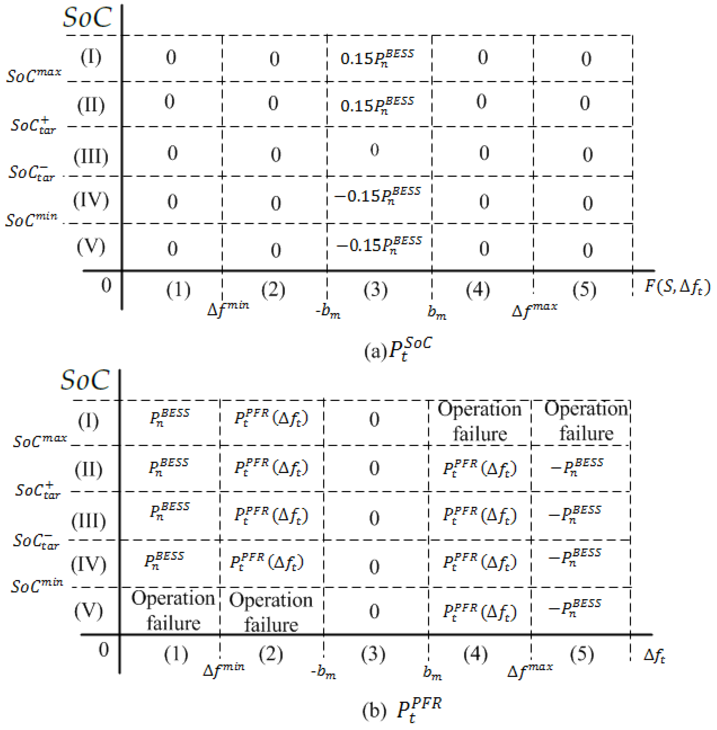
Figure 2 explains how $P_t^{SoC}$ (Figure 2a) and $P_t^{PFR}$ (Figure 2b) powers are calculated according to the regions defined in Figure 1. It is assumed a positive sign for power delivered from BESS to the grid (discharge) and negative for power absorbed by the BESS from the grid (charge). In Figure 2b, $P_t^{PFR}\left(\Delta f_t\right)$ is the portion of power that reacts in a linear fashion with respect to frequency deviations and is given by Equation (1). A positive sign in $b_m$ applies when frequency deviation is positive, while a negative sign applies when frequency deviation is negative.

$$P_t^{PFR}\left(\Delta f_t\right)=\frac{-1}{S·f_n}\left(\Delta f_t\pm b_m\right)$$

(1)

Notice that $P_t^{SoC}$ is allowed to be different from zero only when the grid frequency lies in the deadband region (3). In this sense, $P_t^{SoC}$ can be understood as a sudden load or injection of power to the system depending on its sign. If its magnitude is not small enough, it could cause imbalance between power generation and demand, which in turn could eventually produce further frequency deviations. Therefore, to avoid these perturbations in the system, $P_t^{SoC}$ is assumed to be at most a small percentage $\gamma$ of BESS nominal power $P_n^{BESS}$.

The proposed BESS operation model does not take into account limitations due to the battery charger or BMS (Battery Management System) operation. Previous works like [18,19] considered current and voltage profiles that must be met to guarantee battery safety and health during battery charge operations. Thus, power absorption can be, at certain times, limited to a value lower than that specified by $P_t^{SoC}$ or $P_t^{PFR}$. These limitations are not considered in this work.

3. Proposed Optimization Model for BESS Sizing

The proposed optimization model is aimed to find both the best BESS storage capacity $E_n$ and operation set points $So{C}_{tar}^{-}$ and $So{C}_{tar}^{+}$. One of the criteria used to achieve satisfactory BESS size for PFR is investment cost. Thus, the authors of this paper have assembled this optimization model aimed to find both a cost-effective BESS size that guarantees the proper PFR service and SoC set points that guide the BESS operation in real time. To do so, the SoC dynamics, via difference equations, is modeled using short integration periods that allow capturing frequency deviation dynamics. Two of the key input parameters of the model are $So{C}^{min}$ and $So{C}^{max}$ since they allow tuning the model according to the results of the performance assessment model. It is important to clarify that the key aspects of BESS that are relevant to this formulation are power exchange and energy storage. These parameters define the ability (or inability) to offer a proper PFR service. Although the type of battery and its associated chemistry process are relevant from a construction and design point of view, they are not part of the inputs of the proposed BESS sizing strategy for PFR purposes. The mathematical model is given by the objective function (2) and Constraints (3)–(11).

$$\begin{array}{cc}\mathrm{minimize}\hfill & f_0=I·E_n+\lambda \sum _{t=1}^T{p}_t,\hfill \end{array}$$

(2)

$$\begin{array}{cc}\mathrm{subject}\mathrm{to}\hfill & p_t\ge m_1\left(E_t-E_{tar}^{+}\right),\forall t=1,\dots ,T,\hfill \end{array}$$

(3)

$$\begin{array}{c}{p}_t\ge (m_1-m_2)(So{C}^{max}-0.1)E_n-m_1{E}_{tar}^{+}+m_2{E}_t,\forall t=1,\dots ,T,\hfill \end{array}$$

(4)

$$\begin{array}{c}{p}_t\ge -m_1(E_t-E_{tar}^{-}),\forall t=1,\dots ,T,\hfill \end{array}$$

(5)

$$\begin{array}{c}{p}_t\ge -(m_1-m_2)(So{C}^{min}+0.1)E_n+m_1{E}_{tar}^{-}-m_2{E}_t,\forall t=1,\dots ,T,\hfill \end{array}$$

(6)

$$\begin{array}{c}{P}_t^{PFR}=P_n^{G}max\left(0,min\left(\rho ,\frac{-1}{S·f_n}\left(\Delta f_t+b_m\right)\right)\right)\hfill \\ +P_n^{G}max\left(0,min\left(-\rho ,\frac{-1}{S·f_n}\left(\Delta f_t-b_m\right)\right)\right),\hfill \end{array}$$

(7)

$$\begin{array}{c}{E}_t=E_{tar}^{-}·{\mathbf{1}}_{\left\{t=1\right\}}+E_{t-1}·{\mathbf{1}}_{\left\{t\ge 1\right\}}+\Delta t\left(P_t^{SoC}+P_t^{PFR}\right),\forall t=1,\dots ,T,\hfill \end{array}$$

(8)

$$\begin{array}{c}{E}_{tar}^{+}-E_{tar}^{-}\le {\rho }_{gap}{E}_n,\hfill \end{array}$$

(9)

$$\begin{array}{c}So{C}^{min}{E}_n\le E_t\le So{C}^{max}{E}_n,\forall t=1,\dots ,T,\hfill \end{array}$$

(10)

$$\begin{array}{c}|P_t^{SoC}|\le \gamma P_n^{BESS}{\mathbf{1}}_{\left\{-b_m\le \Delta f_t\le b_m\right\}},\forall t=1,\dots ,T.\hfill \end{array}$$

(11)

The optimal BESS dimension is obtained by minimizing its investment cost and the penalty function, as shown in Equation (2). I represents the unitary investment cost in $/MWh of storage capacity; thus, the product $I·E_n$ is the total BESS cost in $. $p_t$, a convex and piecewise affine function that is illustrated in Figure 3, penalizes SoC deviations during period t from its target band as described in Equations (3)–(6). $m_1$ and $m_2$ ($m_1<m_2$) are the slopes of $p_t$. The set of inequalities (3)–(6) was employed to describe the convex function $p_t$. This is a common strategy in convex optimization formulations and can be understood as the epigraph of the function. To address additional convex optimization concepts, the interested reader can refer to the textbook [20].

Parameters $So{C}^{min}$ and $So{C}^{max}$ represent SoC hard limits, i.e., during the optimization, the BESS is not allowed to operate outside the interval $\left[So{C}^{min},So{C}^{max}\right]$. Furthermore, the resulting SoC target band is defined by interval $\left[So{C}_{tar}^{-},So{C}_{tar}^{+}\right]$. These bounds are related to decision variables $E_{tar}^{-}=So{C}_{tar}^{-}{E}_n$ and $E_{tar}^{+}=So{C}_{tar}^{+}{E}_n$ (in MWh), which in turn define the lower and upper bounds of the target storage level, respectively.

As depicted in Figure 3, $p_t$ penalizes the objective function when either $E_t<E_{tar}^{-}$ or $E_t>E_{tar}^{+}$; and $p_t$ is even larger as long as $E_t$ approaches either $So{C}^{min}{E}_n$ or $So{C}^{max}{E}_n$. In case $E_{tar}^{-}\le E_t\le E_{tar}^{+}$, $p_t$ is zero. This function is constructed with the purpose of maintaining SoC far enough from its limits ($So{C}^{min}$ and $So{C}^{max}$), not only in the optimization model, but also during the PFR assessment, as will be discussed later in Section 4.

Constraint (7) allows computing $P_t^{PFR}$ in terms of frequency deviation $\Delta f_t$, as illustrated in Figure 1a. The slope of linear segments depends on the system frequency regulation constant (or frequency droop) S, nominal frequency $f_n$, deadband ($2b_m$), and $P_n^G$. Signal $P_t^{PFR},t=1,\dots ,T$ does not belong to the decision variable set, but it is a signal resulting from the power system dynamics. In general terms, $P_t^{PFR}$ is the power for the PFR service and is computed such that 1 MW of power should cause a relative change in frequency S between 4% and 6% with respect to its nominal value $f_n$.

A stored energy update is performed according to Constraint (8). This constraint is nothing but a difference equation representing energy storage as the integral of net power handled by the BESS. Indicator function ${\mathbf{1}}_{\left\{x\in A\right\}}$ is one whenever $x\in A$, and zero otherwise. The initial condition assumes that the storage level is at $E_{tar}^{-}$. Energy stored $E_t$ is updated as a result of successive charge and discharge signals throughout the analysis horizon. When $-b_m\le \Delta f_t\le b_m$, frequency is located in Region 3 of Figure 1a, which indicates that the BESS enters into either a charging or discharging process. This process is developed to return storage level $E_t$ to the target band given by $\left[E_{tar}^{-},E_{tar}^{+}\right]$ (this is equivalent to returning SoC to its target band given by $\left[So{C}_{tar}^{-},So{C}_{tar}^{+}\right]$) by the proper values of $P_t^{SoC},t=1,\dots ,T$.

The storage target band is parameterized in Constraint (9) in terms of a percentage ${\rho }_{gap}$ of storage capacity $E_n$. This constraint basically states that the width of the gap (measured in units of energy) cannot be larger than a small percentage of the nominal storage capacity. In any case, stored energy $E_t$ cannot operate outside the operational limits $So{C}^{min}{E}_n$ and $So{C}^{max}{E}_n$ as suggested by the restrictions (10).

Power signal $P_t^{SoC},t=1,\dots ,T$ represents a key decision variable in this model. It allows managing SoC at times when frequency is under the normal condition. The constraints (11) state that $P_t^{SoC}$ needs to be at most a percentage $\gamma$ of BESS nominal power. Note that $P_t^{SoC}$ can be either positive or negative, i.e., it can represent charge or discharge only when frequency deviations are small. The model chooses the magnitude of $P_t^{SoC}$ according to the “distance” of current SoC to its target band during period t.

4. BESS Performance Assessment Algorithm

A performance assessment algorithm is proposed to emulate BESS operation using a predefined frequency dataset. The assessment goal is to compute performance indexes such as penalization costs, battery lifetime, battery replacements, and SoC target band. The outputs of the optimization model ($E_n,So{C}_{tar}^{-},So{C}_{tar}^{+}$) represent the input parameters to the performance assessment algorithm. This algorithm is presented as a two-step process:

4.1. Step 1: Continuous SoC Estimation

The goal of this step is to estimate SoC and penalization counts using the entire dataset of frequency deviations. To do so, both $P_t^{PFR}$ and $P_t^{SoC}$ are computed using frequency deviation from the dataset, current SoC, and the droop characteristic, as described in Figure 1 and Figure 2. This is analogous to restrictions (7) and (11) presented in Section 3.

Then, an energy balance (resulting from the integral of net power $P_t^{PFR}+P_t^{SoC}$) is proposed to update the stored energy at the end of period t using Equation (12).

$$E_t=E_{t-1}+(P_t^{PFR}+P_t^{SoC})\Delta t,\forall t=1,\dots ,T$$

(12)

Likewise, the corresponding SoC is updated by dividing both sides of Equation (12) by $E_n$ as presented in (13):

$$So{C}_t=So{C}_{t-1}+\frac{(P_t^{PFR}+P_t^{SoC})\Delta t}{E_n},\forall t=1,\dots ,T$$

(13)

To estimate BESS battery lifetime, $E_t^{circ}$ needs to be calculated. $E_t^{circ}$ is understood as the energy that has circulated in the battery up to period t, regardless whether it is caused by charge or discharge processes. It is computed using Equation (14):

$$E_t^{circ}=E_{t-1}^{circ}+\left(\left|P_t^{PFR}\right|+\left|P_t^{SOC}\right|\right)\Delta t,\forall t=1,\dots ,T$$

(14)

A penalization is considered whenever SoC is in Region (V) and frequency deviation in Regions (1) or (2), or when SoC is in Region (I) and frequency deviation in Regions (4) or (5). These cases represent BESS failing to provide PFR service due to either BESS overcharge or over-discharge, which are considered as over-frequency and low-frequency penalization, respectively. This is depicted at the bottom-left and top-right corners of Figure 2b. The number of days with at least one over-frequency penalty is represented by $N^{+}$; whereas the number of days with at least one low-frequency penalty is $N^{-}$. The process of assessing the failure-to-provide-PFR is carried out continuously and will finally return the total number of penalty days with at least one penalization $N=N^{+}+N^{-}$.

4.2. Step 2: Performance Indexes’ Computation

Once Step 1 has been completed, penalization costs, battery lifetime, battery replacements, and investment costs need to be computed. Given that the total number of penalization days N is valid for the analysis horizon defined by the available frequency dataset, it is necessary to extrapolate N over the solar plant’s lifetime, namely $N^{life}$. Assuming a similar behavior for frequency and BESS during the solar plant lifetime, such an extrapolation is given by:

$$N^{life}=\left(\frac{T_{sol}}{T_{asm}}\right)N$$

(15)

where $T_{sol}$ is the estimated lifetime for the solar plant and $T_{asm}$ refers to the amount of time covered in the available frequency dataset. The selected criterion for computing penalization cost $C^{pen}$ is adapted from the Colombian PFR regulation [21] and shown in Equation (16). It is worth mentioning that any other criterion for cost penalties when PFR is not properly offered can be easily assembled with this methodology.

$$C^{pen}=2G_R\rho p_{pen}{N}^{life}$$

(16)

$G_R$ represents the total estimated energy generation for the solar plant in a 24-h period; $\rho$ is the percentage of PFR reserve for the plant; and $p_{pen}$ is the penalization price. However, the proposed BESS sizing strategy in this work is flexible enough to accommodate other penalization cost criteria.

In this work, a solar plant with an installed power capacity given by $P_n^G$ and an average capacity factor given by $CF$ is assumed. $CF$ is known as the ratio of total electricity generated to the maximum energy that a power plant can produce at continuous full-power operation [22]. Thus, it is the estimated average daily energy production ($G_R$) is given by:

$$G_R=24CF{P}_n^G$$

(17)

BESS battery lifetime is calculated by using the energy throughput model presented in [23,24] and as presented in Equation (18):

$$T_{BESS}=\left(\frac{E^{th}}{E_T^{circ}}\right)T_{asm}$$

(18)

$E_T^{circ}$ represents the battery wear during the analysis horizon time $T_{asm}$ and refers to the the final point of the energy circulating trajectory $E_t^{circ},t=1,\dots ,T$ presented in Equation (14). This lifetime model assumes a given amount of energy $E^{th}$ that the battery can exchange (during charge or discharge) before reaching its lifetime. According to the works [23,24], $E^{th}$ can be computed from the battery manufacturer curves that represent the number of cycles $C_f$ as a function of average depth of discharge $DoD$. However, in this paper, $E^{th}$ is calculated using Equation (19), which corresponds to lead-acid batteries. Nevertheless, the authors of this paper do not pretend to limit the range of application of this methodology to lead-acid batteries only. For other battery technologies, $E^{th}$ can be estimated using the approaches presented in [4,25].

$$E^{th}=DoD{E}_n{C}_f$$

(19)

Optimal BESS sizing for PFR purposes requires the evaluation of performance in operation. A BESS with low energy capacity ($E_n$) has low initial investment costs; but in the end, it can be more expensive if additional investment costs over the lifetime of the solar project are considered due to future replacements. Thus, for a more realistic economic evaluation, the number of BESS replacements $N_r$ during the solar plant lifetime needs to be calculated. To do so, Equation (20) is employed:

$$N_r=⌈\frac{T_{sol}}{T_{BESS}}⌉$$

(20)

where $⌈x⌉$ indicates the least integer that is greater than or equal to x. Thus, $N_r$ indicates how many BESS need to be invested in in order to fully cover the power plant’s lifetime period. Finally, total BESS investment and replacement costs are calculated as follows:

$$C^I=I{E}_n{N}_r$$

(21)

The final decision regarding the optimal BESS size is chosen as the one that minimizes the total project cost given by $C^{pen}+C^I$.

5. Results

In order to test both the optimization model and the assessment algorithm, a $P_n^G=$10 MW solar PV power plant with a $CF$ = 20% capacity factor was considered. Lifetime was assumed to be $T_{sol}$ = 25 years. As mentioned earlier, the BESS was designed entirely for providing PFR service to which the solar PV plant was committed. $\rho =3$% of the plant capacity had to be dedicated for frequency control, which means the nominal BESS power was $P_n^{BESS}=0.3$ MW. The nominal frequency was $f_n=60$ Hz and the deadband $b_m=30$ MHz. Furthermore, the frequency droop was $S=6$%. BESS investment cost was assumed to be $I=600$ $/kW; this is considering the battery management system and power conversion system. An SoC target bandwidth of ${\rho }_{gap}$ = 5% was assumed, and slopes for the penalty function were given by $m_1$ = 40 and $m_2$ = 80. The assumed number of BESS cycles was $C_f$ = 100,000. The percentage of BESS nominal power $\gamma$ to recover its SoC to the target band was assumed to be 15%. Since nominal power was 300 kW, $\left|P_t^{SoC}\right|$ was bounded by 45 kW in order to prevent posterior frequency deviations.

Frequency event data were provided by the Colombian Independent System Operator (ISO) called XM. It contains 10,819,703 frequency records, sampled every four seconds by a Phasor Measurement Unit (PMU), and they were collected between December 2014 and April 2016. However, a sample of one million data points was considered in the optimization model described in Section 3. The performance assessment algorithm used the entire set of available data.

The resulting linear program presented in Section 3 was solved using GAMS (24.4.6, GAMS Development Corporation, Washington, DC, USA) and took one hour on average using a 3.3-GHz, 64-GB workstation; whereas the performance assessment algorithm was coded using MATLAB (R2014a, Mathworks, Natick, MA, USA), and the average CPU time was 10 min.

5.1. Frequency Events’ Characterization

Figure 4 illustrates the frequency deviation distribution of the data. Frequency deviations ranged between −0.48 Hz and 0.24 Hz; however, 95% of the data oscillated between −0.06 Hz and 0.06 Hz. During 70.22% of the time, the frequency lied in its acceptable range; thus, PFR was required 29.78% of the time. High-frequency events above the deadband were observed 12.5% of the time; whereas low-frequency events occurred 17.28% of the time. Therefore, the frequency distribution implied that BESS would be mostly absorbing power from the grid under PFR service.

Data samples employed for BESS sizing via the optimization model represented a time window capturing the most extreme 47 days (one million data points) of frequency events. Out of these data, 47.22% of the frequency deviations required BESS control action for PFR; 18.83% and 28.39% of the frequency represented high-frequency and low-frequency events.

Figure 5a shows the $P_t^{PFR}$ distribution resulting by employing Equation (7) to the entire dataset. The 95% confidence interval of $P_t^{PFR}$ was $\left[-0.0833,0.0833\right]$ MW. Figure 5b shows $P_t^{PFR}$ for the sample frequency data. According to these distributions, both datasets were statistically similar.

5.2. BESS Sizing

The proposed optimization model was executed under different penalty levels $\lambda$ and different operational parameters $So{C}^{min}$ and $So{C}^{max}$. The optimization model provided storage capacity $E_n$, which is an input to the evaluation algorithm. This algorithm was useful in the sense that it performed BESS assessment under typical operational rules for PFR purposes. The BESS assessment was measured through the number of days in which PFR was not properly carried out. It was called the penalty number N, split into $N^{-}$ and $N^{+}$, representing the number of penalizations in low-frequency and high-frequency events, respectively. Results are described in

Table 1. Optimization and assessment results.

Optimization Parameters			Optimization Output			Assessment
${\mathit{SoC}}^{\mathit{min}}$	${\mathit{SoC}}^{\mathit{max}}$	$\mathit{\lambda }$	${\mathit{E}}_{\mathit{n}}$(MWh)	Target Band (%)		${\mathit{N}}^{+}$	${\mathit{N}}^{-}$	$\mathit{N}$
				${\mathit{SoC}}_{\mathit{tar}}^{-}$	${\mathit{SoC}}_{\mathit{tar}}^{+}$
0.10	0.90	2000	1.23	21.51	26.1	0	0	0
		1000	0.546	25.17	30.17	0	0	0
		667	0.442	27.30	32.30	0	0	0
		500	0.359	29.78	34.78	0	0	0
		333	0.263	34.57	39.57	0	1	1
		60	0.135	46.68	46.68	0	1	1
		6	0.111	47.07	52.07	1	1	2
0.25	0.75	2000	1.23	36.51	41.51	0	0	0
		1000	0.546	40.17	45.17	0	0	0
		667	0.442	42.30	47.30	0	0	0
		500	0.359	44.77	49.77	0	0	0
		333	0.293	47.62	52.62	0	1	1
		60	0.254	47.15	52.15	0	1	1
		6	0.177	47.52	52.52	0	3	3
0.30	0.70	2000	1.23	41.51	46.51	0	0	0
		1000	0.546	45.17	50.17	0	0	0
		667	0.443	47.26	52.26	0	0	0
		500	0.435	47.20	52.20	0	1	1
		333	0.424	47.13	52.13	1	0	1
		60	0.373	46.96	51.96	0	1	1
		6	0.221	47.76	52.76	5	0	5

.

As observed in Table 1, there was a clear dependence between BESS size and penalty level $\lambda$. As long as $\lambda$ increased, BESS sizing was also bigger. Penalty function $p_t$ became more important in the objective function (Equation (2)) whenever $\lambda$ increased; then, $SoC$ was less able to approach its operational limits $So{C}^{min}$ and $So{C}^{max}$ during PFR. To do so in practical terms, BESS storage capacity $E_n$ needs to be large enough such that its energy storage level remains within the target band. The opposite occurred as long as $\lambda$ decreased, since investment cost tended to prevail over penalty $p_t$. 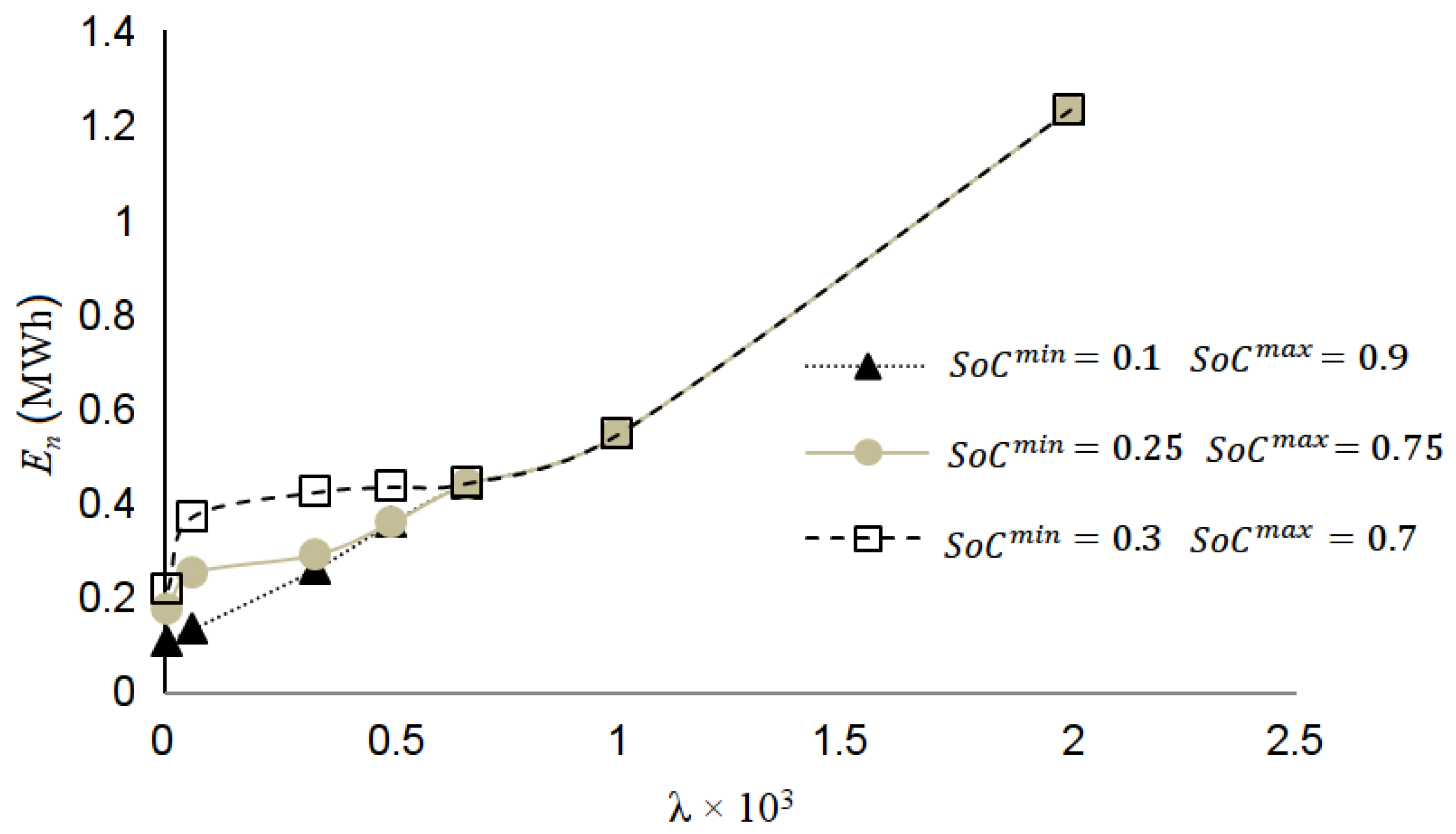A graphical representation of BESS size vs. penalty under different SoC bounds is provided in Figure 6. If $\lambda >700$, there was no perceived effect of SoC bounds on BESS size given that $p_t$ was too large to prevail over investment cost. For lower values of $\lambda$, tighter SoC bounds led to bigger BESS sizes in order to avoid penalization during the charging and discharging process in PFR. These bounds are hard constraints that need to be satisfied at anytime.

5.3. Penalization

Results in Table 1 also provide the number of penalizations caused by different BESS sizes. The 221-kWh BESS ($0.3\le SoC\le 0.7$) displayed the worst performance against high frequency events, i.e., under the excess of generation in the system. This means that when sudden positive frequency deviations occurred, SoC was close to 70%, and BESS could not absorb the additional power required for PFR. According to the results, this situation was observed during five days in the dataset.

Additionally, the larger the BESS sizing, the lower the penalization levels N. The resulting 111-kWh BESS (when $\lambda$ = 6) yielded one penalization in PFR under, both for low-frequency and high-frequency events. However, the 135-kWh/300-kW BESS (when $\lambda$ = 60) yielded only one penalization in PFR under low-frequency events. SoC target band location also played a key role in affecting BESS performance. In fact, even the 359-kWh BESS displayed a zero penalization level when the SoC target band was within 29.78% and 34.78%. Indeed, as depicted in Table 1, even for a BESS with a fixed size $E_n$, N could change. The SoC target band was also a decision made by the proposed model; but, based on the findings of this work, it is essential to have an assessment tool (as described in Section 4) that provides realistic performance measures useful for determining the best SoC target band. The reason is that from the optimization model perspective, it is not possible to know the frequency signal in advance.

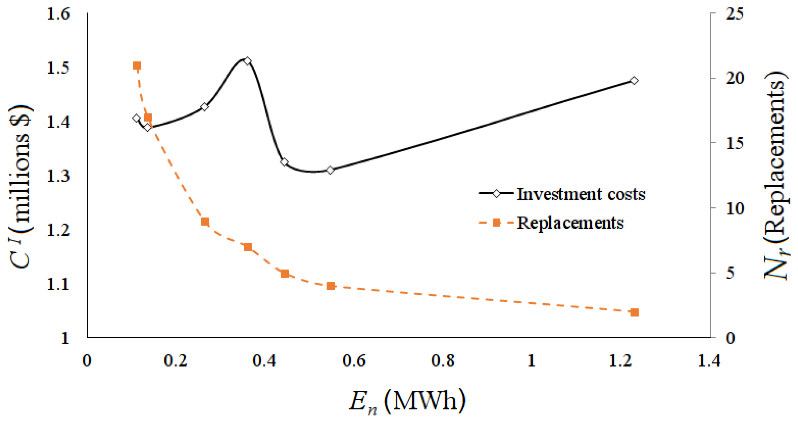
5.4. Investment Costs

In order to evaluate BESS investment cost, Figure 7 is presented. If BESS replacements were neglected, the investment costs curve would be linear with slope I. Figure 7 also shows how the number of BESS replacements $N_r$ dramatically increased as long as $E_n$ decreased. These results were obtained once the lifetime was computed as presented in Equations (18) and (20). In fact, if $E_n=300$ kWh, the lifetime was four years according to the performance assessment algorithm, and thus, seven replacements are needed in order to fully provide PFR during the 25-year period. This explains the increment in investment cost in Figure 7. $N_r$ tended to increase since the charging and discharging process was more intense as long as the BESS size was smaller. From the total investment cost perspective, the 546-kWh BESS was the most cost-effective alternative. It is estimated that such a BESS design would require four replacements throughout the solar plant’s lifetime.

5.5. Penalization Cost

Three scenarios of penalization cost were considered: $p_{pen}=33.33$ $/MWh, $66.67$ $/MWh, and 100 $/MWh. These represent the typical power spot price observed in the Colombian power market [26]. Penalization costs are computed once penalties ($N,N^{-},N^{+}$) are found using the performance assessment algorithm presented in Section 4.

Penalization cost results are illustrated in Figure 8. A BESS with reduced storage capacity implies high penalization cost. For capacities around 110 kWh, the cost was over $20,000 during the 25-year period. Nevertheless, this is significantly lower—by several orders of magnitude—than the corresponding investment cost (displayed in Figure 7). An important fact is that a 546-kWh BESS or higher does not incur a penalization cost, i.e., this BESS always provides PFR satisfactorily.

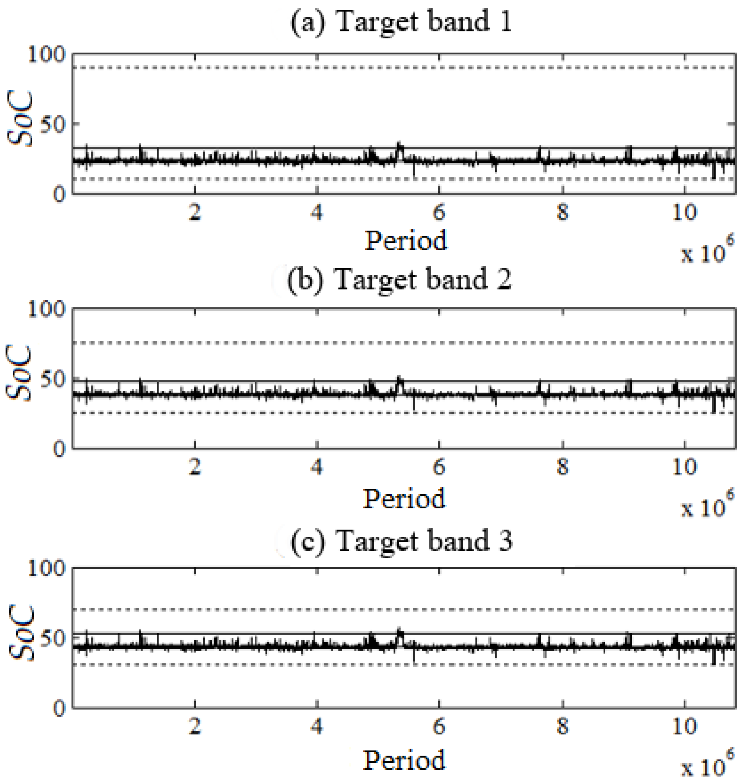
The SoC performance of the 546-kWh BESS under different SoC target bands is presented in Figure 9. Dotted horizontal lines represent the SoC limits ($So{C}^{max}$, $So{C}^{min}$), while continuous horizontal lines are the target SoC band limits ($So{C}_{tar}^{+}$, $So{C}_{tar}^{-}$). Each of these target bands are the product of the optimization model using 47 days of data. The target band in Figure 9a is $\left[25.2\%,30.2\%\right]$, in Figure 9b is $\left[40.2\%,45.2\%\right]$, and in Figure 9c is $\left[45.2\%,50.2\%\right]$. Based on these results, the resulting SoC lies most of the time in the corresponding target bands. This empirical evidence highlights the effectiveness of function $p_t$, which is minimized in the objective function (2).

6. Conclusions

In conclusion, storage capacity, as well as operational criteria provided by the optimization model lead to significant low penalty levels when BESS is assessed in PFR. It was also found that lower and upper bounds of SoC impact BESS sizing as long as the penalty level $\lambda$ decreases, the tighter the bounds, the bigger the BESS. The impact is negligible when $\lambda$ is high. As a general remark, $\lambda >500$ led to BESS designs with zero penalty levels assuming the aforementioned investment cost and parameters.

Furthermore, in order to find satisfactory BESS sizing alternatives, it is crucial to extract a subset of data properly—maintaining chronological order—with the most “extreme” frequency events. By doing so, not only is the optimization model lighter than the model constructed with the entire dataset, but the resulting sizing alternatives perform well in operation mode.

Additionally, in financial terms, assessing BESS performance during the solar plant’s lifetime allows finding a better estimation of the total BESS investment cost. This cost should consider the number of BESS replacements according to the operation behavior and charge/discharge patterns, which are essentially random in PFR. The process of computing the number of replacements is supported by a degradation model that considers these patterns. Otherwise, the optimal BESS size would be smaller.

All in all, the resulting optimal BESS size balances investment and penalization cost under failure in supporting PFR. Since the operational performance was assessed with 4-s sampled data covering more than 15 months, and it is guaranteed that the optimal BESS size can perform satisfactorily under a great variety of frequency disturbances. In general, the proposed methodology was carefully constructed and assembled to provide meaningful, practical, and applicable results in terms of proper size of BESS dedicated to providing the PFR service for which solar power plants are responsible. Most importantly, the proposed strategy for sizing of the BESS that supports PFR of solar power plants is simple and can be applied by industries and companies involved in the integration of renewable energy to power grids.