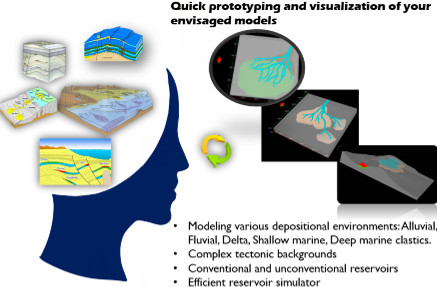
Static Geological Modelling with Knowledge Driven Methodology

Abstract
:
1. Introduction
2. Knowledge Driven Methodology
2.1. Modelling Basis: Understanding from Perspective of Geologists
2.2. 2D Sketch for 3D Facies Models
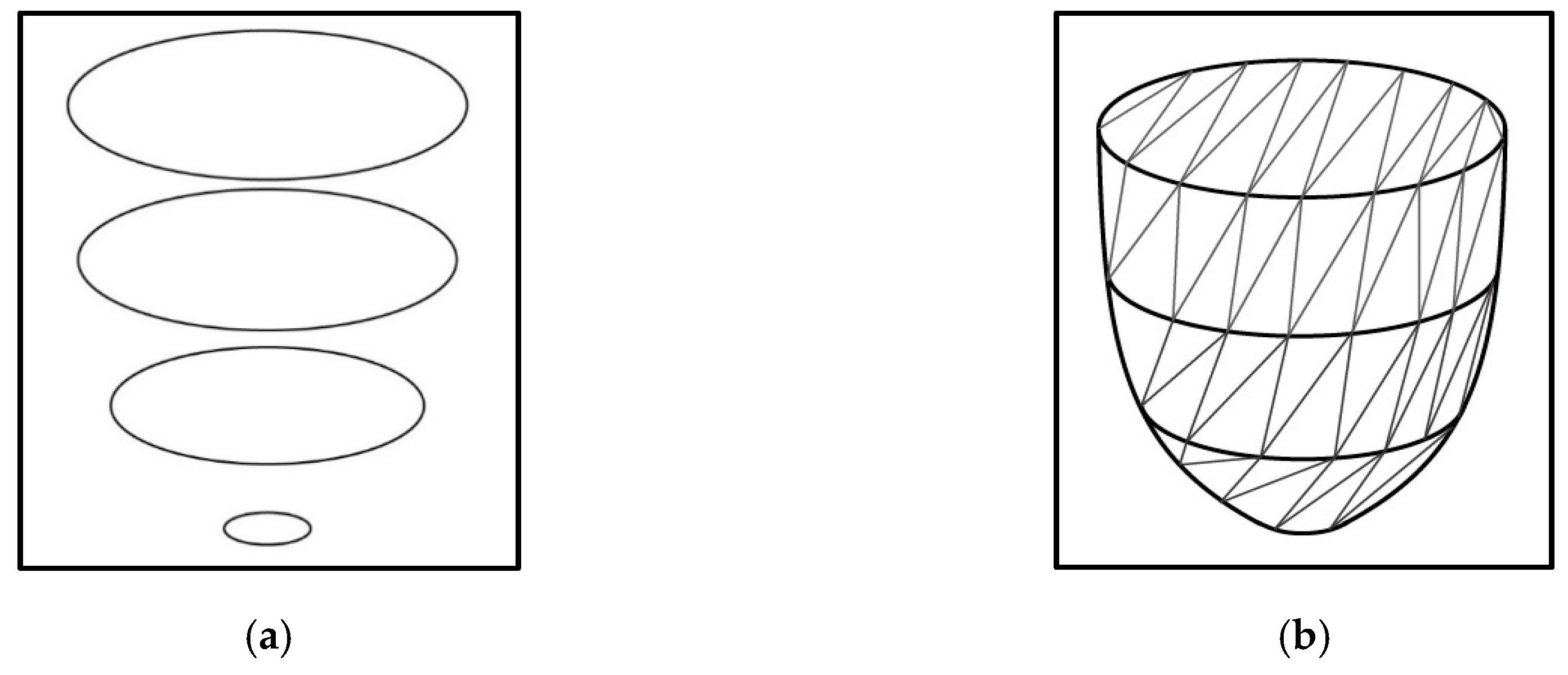
2.2.1. Modelling Algorithm
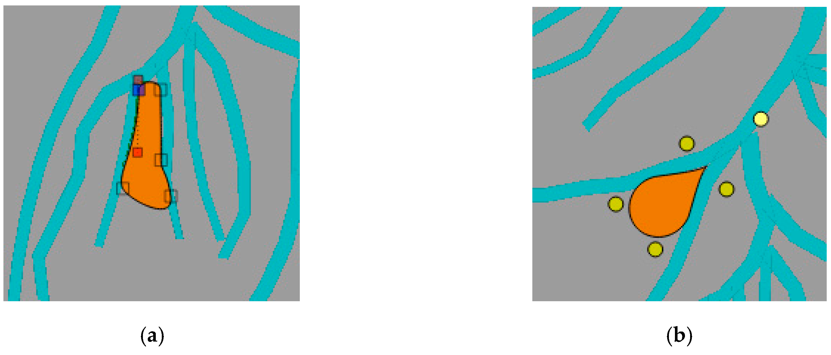
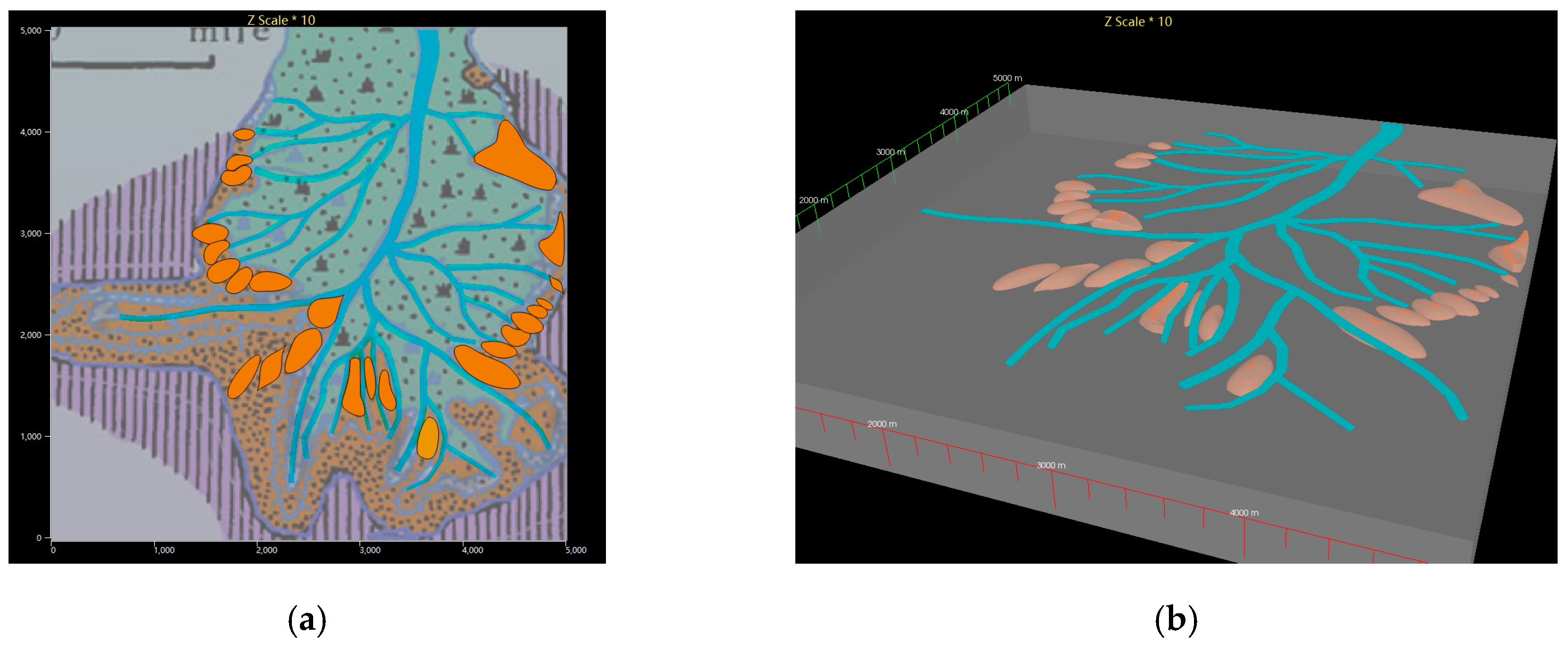
2.2.2. Belt Sand-Bodies
2.2.3. Non-Belt Sand-Bodies
2.2.4. Carbonate Reefs
2.3. Structure Modelling
2.4. Model Library
3. Illustration of DMatlas Modelling Process
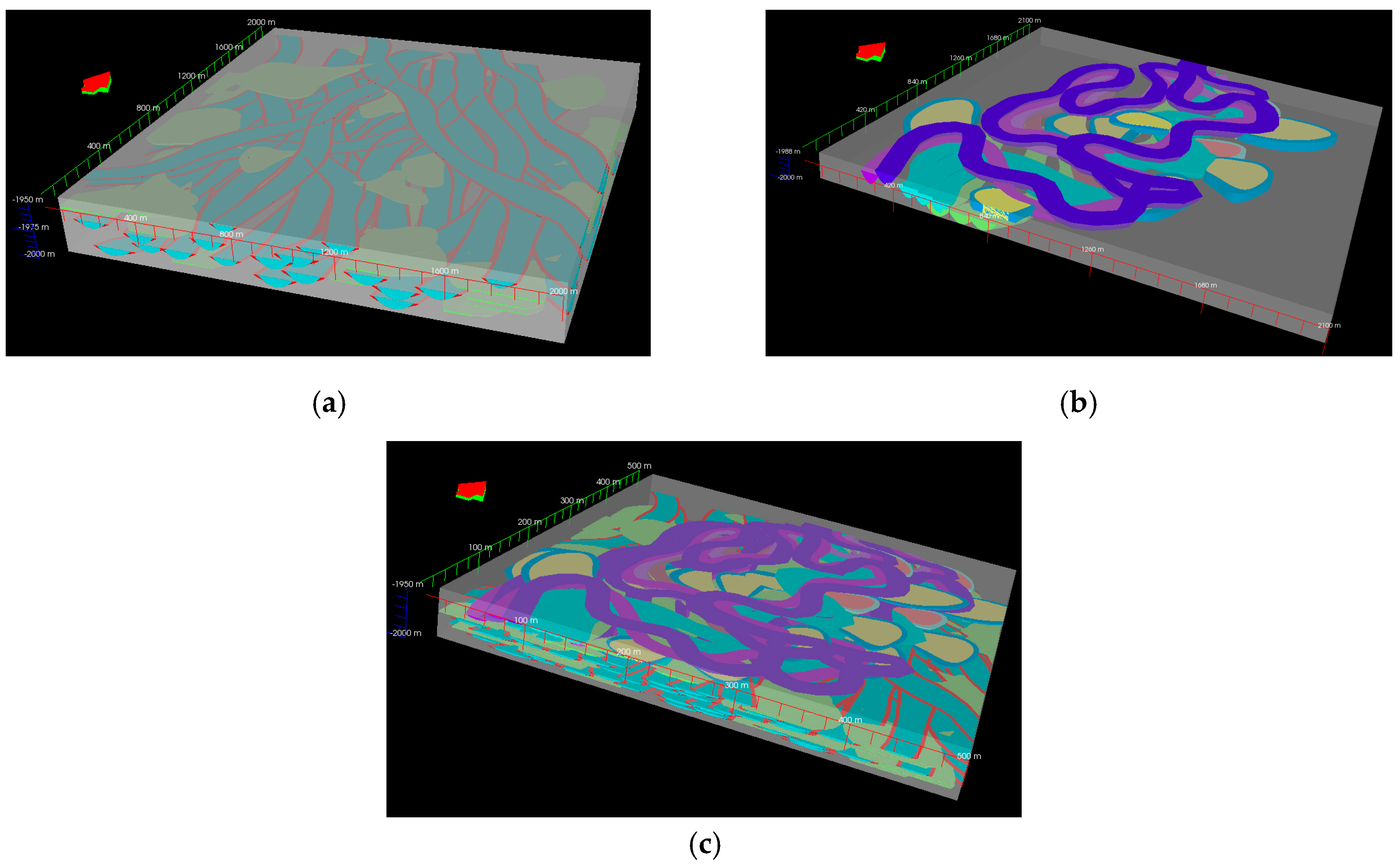
3.1. Fluvial Environment
3.2. Delta Environment
3.3. Shallow Marine Carbonate
3.4. Fault, Folds, and DFN
3.5. Property Modelling
3.6. Export of A Model
4. Case Studies
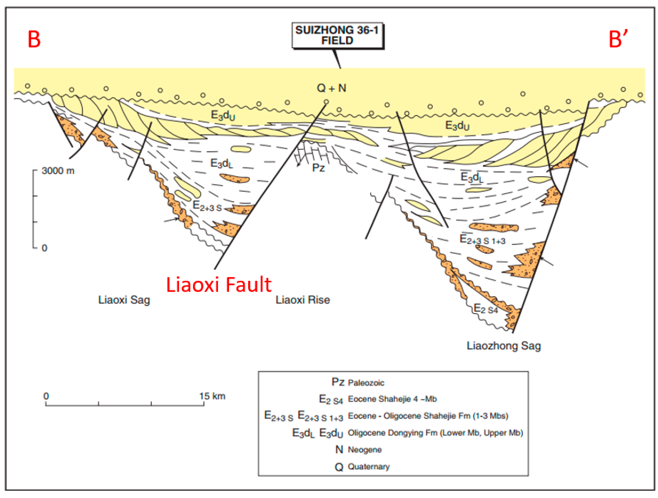
4.1. SZ 36-1 Field
4.1.1. Geologic Background
4.1.2. Facies Modelling
4.1.3. Variable Thickness
4.1.4. Liaoxi Fault
4.1.5. Petrophysical Properties Modelling
4.1.6. Volume Calculation Result from Dmatlas
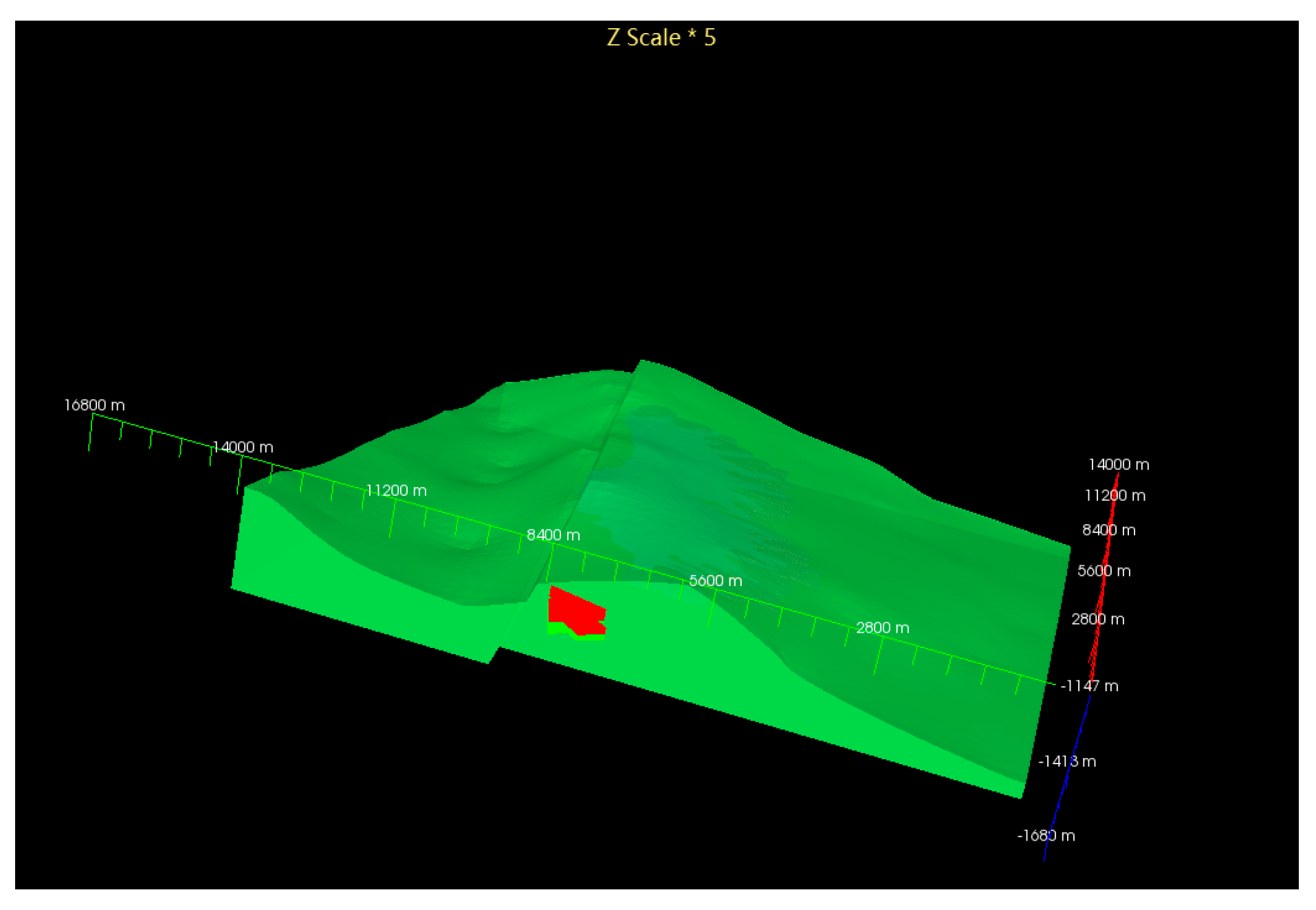
4.2. The North Oman Fracture System
4.2.1. Geologic Background of the Natih Formation, Jebel Madmar
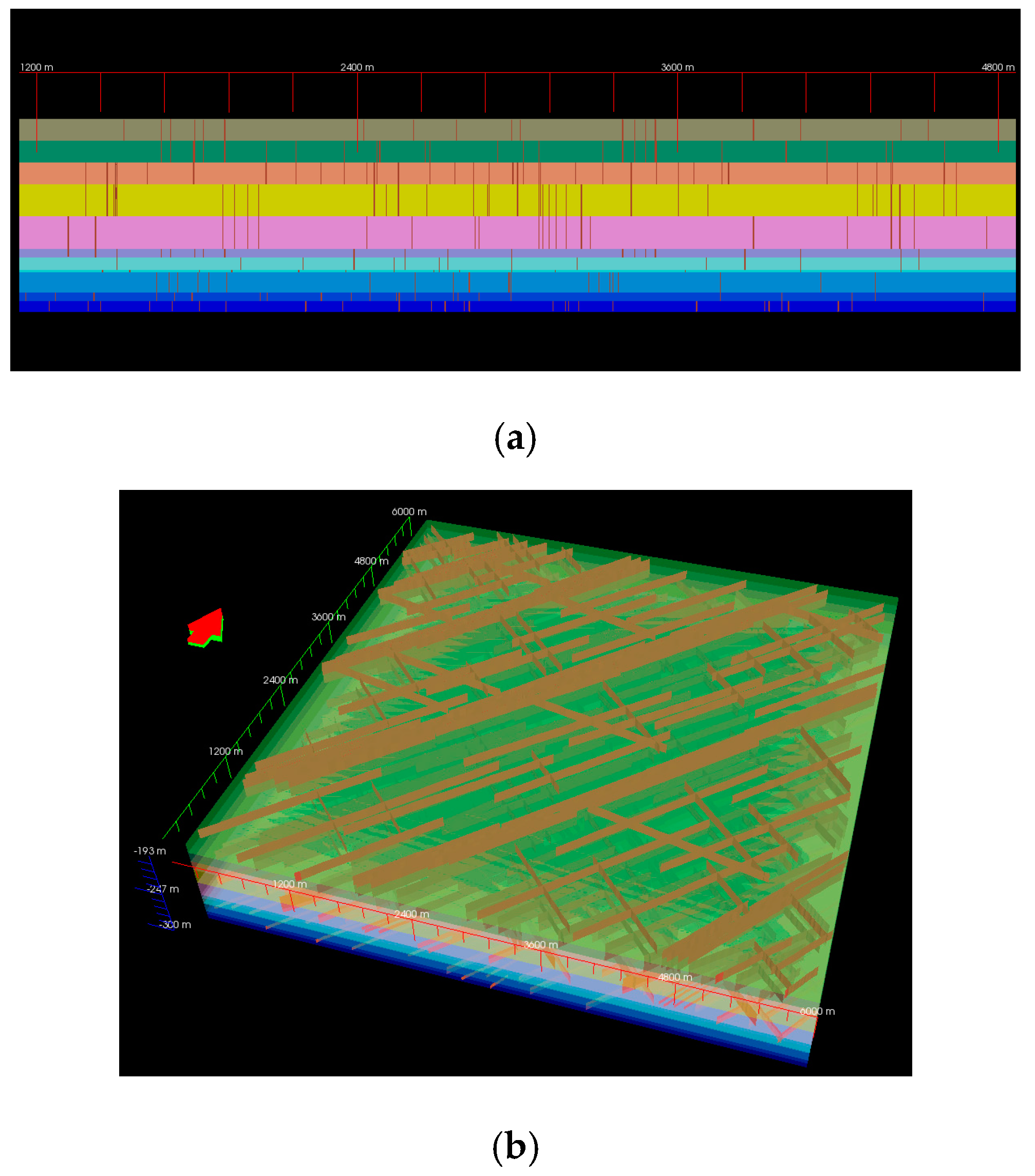
4.2.2. Fractures Modelled by DMatlas
- A sector scale of 6000 × 6000 m area on the back-limb of Madmar anticline.
- Made up of the sets that dominate subsurface structure in the region at the well- and inter-well scales: WNW normal faults, NW fractures, and NE regional fractures, as well as subordinate northerly trending structures.
- 11 upscaled main mechanical stratigraphy are established in total for Natih E.
- Fractures and corridors with vertical dips.
- Fracture width, fault throw and other structures (e.g., low-angle thrusts) are not in the model.
5. Conclusions
Author Contributions
Funding
Acknowledgments
Conflicts of Interest
References
- Fanchi, J.R. Chapter 2—Geological modeling. In Principles of Applied Reservoir Simulation, 4th ed.; Fanchi, J.R., Ed.; Gulf Professional Publishing: Houston, TX, USA, 2018; pp. 9–33. [Google Scholar]
- Howell, J.A.; Martinius, A.W.; Good, T.R. The application of outcrop analogues in geological modelling: A review, present status and future outlook. Geol. Soc. Lond. Spec. Publ. 2014, 387, 1–25. [Google Scholar] [CrossRef]
- Schlumberger. Petrel Structural Modeling Training and Exercise Guide; Schlumberger: Houston, TX, USA, 2014. [Google Scholar]
- Li, J.; Li, X. Analysis of u-tube sampling data based on modeling of CO2 injection into CH4 saturated aquifers. Greenh. Gases Sci. Technol. 2015, 5, 152–168. [Google Scholar] [CrossRef]
- Sech, R.P.; Jackson, M.D.; Hampson, G.J. Three-dimensional modeling of a shoreface-shelf parasequence reservoir analog: Part 1. Surface-based modeling to capture high-resolution facies architecture. AAPG Bull. 2009, 93, 1155–1181. [Google Scholar] [CrossRef]
- Deveugle, P.E.K.; Jackson, M.D.; Hampson, G.J.; Stewart, J.; Clough, M.D.; Ehighebolo, T.; Farrell, M.E.; Calvert, C.S.; Miller, J.K. A comparative study of reservoir modeling techniques and their impact on predicted performance of fluvial-dominated deltaic reservoirs comparison of reservoir modeling techniques. AAPG Bull. 2014, 98, 729–763. [Google Scholar] [CrossRef]
- Li, S.; Zhang, Y.; Ma, Y.Z.; Dorion, C.; Daly, C.; Zhang, T. A comparative study of reservoir modeling techniques and their impact on predicted performance of fluvial-dominated deltaic reservoirs: Discussion. AAPG Bull. 2018, 102, 1659–1663. [Google Scholar] [CrossRef] [Green Version]
- Perrin, M.; Zhu, B.T.; Rainaud, J.F.; Schneider, S. Knowledge-driven applications for geological modeling. J. Pet. Sci. Eng. 2005, 47, 89–104. [Google Scholar] [CrossRef]
- Mehran, M.H.; Michael, J.P.; Clayton, V.D. Improved geostatistical models of inclined heterolithic strata for McMurray Formation, Alberta, Canada. AAPG Bull. 2013, 97, 1209–1224. [Google Scholar]
- Crama, Y.; Hammer, P.L. Boolean Functions: Theory, Algorithms, and Applications; Cambridge University Press: Cambridge, UK, 2011. [Google Scholar]
- Ferguson, R.S. Practical Algorithms for 3d Computer Graphics, 3nd ed.; Routledge: Abingdon, UK, 2014. [Google Scholar]
- Miall, A.D. Reconstructing the architecture and sequence stratigraphy of the preserved fluvial record as a tool for reservoir development: A reality check. AAPG Bull. 2006, 90, 989–1002. [Google Scholar] [CrossRef]
- Fisher, W.L.; Brown, L.F., Jr.; Scott, A.J.; McGowen, J.H. Delta Systems in the Exploration for Oil and Gas; The University of Texas at Austin, Bureau of Economic Geology: Austin, TX, USA, 1969; p. 212. [Google Scholar]
- Tucker, M.E. Shallow-marine carbonate facies and facies models. Geol. Soc. Lond. Spec. Publ. 1985, 18, 147–169. [Google Scholar] [CrossRef]
- Wilson, J.L. Carbonate Facies in Geologic History; Springer: New York, NY, USA, 1975. [Google Scholar]
- Read, J.F. Carbonate platform facies models. AAPG Bull. 1985, 69, 1–21. [Google Scholar]
- Li, Y. The Highly Faulted Oilfield in Wenmingzhai; Petroleum Industry Press: Beijing, China, 1997; p. 140. [Google Scholar]
- Price, N.J. Fault and Joint Development in Brittle and Semi-Brittle Rock; Pergamon, Turkey, 1966; p. 186. [Google Scholar]
- Yang, H.; Fu, J.; Wei, X.; Liu, X. Sulige field in the Ordos basin: Geological setting, field discovery and tight gas reservoirs. Mar. Pet. Geol. 2008, 25, 387–400. [Google Scholar] [CrossRef]
- Guo, J.L. Study on Relatively Prolific Reservoir Distribution of Sulige Gasfield; China University of Geosciences: Wuhan, China, 2008. [Google Scholar]
- Ran, X.Q.; Li, A.Q. Sulige Gas Development Approach; Petroleum Industry Publishing: Beijing, China, 2008; p. 246. [Google Scholar]
- Zhu, X.; Liu, C. Identification of effective upper paleozoic reservoirs in Sulige area. Nat. Gas Ind. 2006, 26, 1–3. [Google Scholar]
- Schlumberger. Eclipse Reservoir Simulation Software; Schlumberger: Houston, TX, USA, 2012. [Google Scholar]
- King, M.J.; Ballin, P.R.; Bennis, C.; Heath, D.E.; Hiebert, A.D.; McKenzie, W.; Rainaud, J.-F.; Schey, J. Reservoir modeling: From rescue to RESQML. SPE Reserv. Eval. Eng. 2012, 15, 127–138. [Google Scholar] [CrossRef]
- Verney, P.; Gautreau, C.; Rainaud, J.-F.; Deny, L.; Magsipok, J.; Marcotte, D. RESQML version 2 uses new technologies to improve data exchange for subsurface modeling processes. In SPE Intelligent Energy Conference & Exhibition; Society of Petroleum Engineers: Utrecht, The Netherlands, 2014; p. 11. [Google Scholar] [CrossRef]
- Xin, S.G.; Li, Y.Q.; Ding, K.W. Exploration Practice in Major Oilfields of China; Petroleum Industry Press: Beijing, China, 2002. [Google Scholar]
- Xin, S.G.; Hao, F.G.; Li, Y.Q.; Ding, K.W. Major Non-Marine Oil Fields of China; Petroleum Industry Press: Beijing, China, 1997. [Google Scholar]
- Xin, S.G.; Luedke, D.K. Field development of the Suizhong 36-1 oil field using geophysics and reservoir simulation. SEAPEX Proc. 1990, 9, 121–132. [Google Scholar]
- Gustavson, J.B.; Xin, S.G. The Suizhong 36-1 oil field, Bohai Gulf, offshore China. AAPG Memoir. 1992, 54, 459–470. [Google Scholar]
- Deng, M.Y.; Zhang, C.Y.; Dong, X.L.; Liu, Z.M.; Liu, Q.H. Evaluation on formation damage by well operation fluid in SZ 36-1 oil field. China Offshore Oil Gas Eng. 2001, 13, 17–24. [Google Scholar] [CrossRef]
- Zhu, X.; Dong, Y.; Yang, J.; Zhang, Q.; Li, D.; Xu, C.; Yu, S. Sequence stratigraphic framework and distribution of depositional systems for the paleogene in Liaodong bay area. Sci. China Ser. D Earth Sci. 2008, 51, 1–10. [Google Scholar] [CrossRef]
- Dai, H.D.; Gong, Z.S. The Development of Offshore Oil-Gas Fields in China; Petroleum Industry Press: Beijing, China, 2003; p. 281. [Google Scholar]
- Bazalgette, L. Relations plissement/fracturation multi échelle dans les multicouches sédimentaires du domaine élastique/fragile: Accommodation discontinue de la courbure par la fracturation de petite échelle et par les articulations. In Possibles Implications Dynamiques dans les Écoulements des Reservoirs; Université Montpellier II-Sciences et Techniques du Languedoc: Montpellier, France, 2004. [Google Scholar]
- De Keijzer, M.; Hillgartner, H.; Al Dhahab, S.; Rawnsley, K. A surface–subsurface study of reservoir-scale fracture heterogeneities in cretaceous carbonates, north Oman. In Fractured Reservoirs; Lonergan, L., Jolly, R.J.H., Rawnsley, K., Sanderson, D.J., Eds.; Geological Society of London: London, UK, 2007. [Google Scholar] [CrossRef]
- Tschopp, R.H. Development of the fahud field. In 7th World Petroleum Congress; World Petroleum Congress: Mexico City, Mexico, 1967; p. 8. [Google Scholar]
- Lei, H.; Li, J.; Li, X.; Jiang, Z. Numerical modeling of co-injection of N2 and O2 with CO2 into aquifers at the Tongliao CCS site. Int. J. Greenhouse Gas Control 2016, 54, 228–241. [Google Scholar] [CrossRef]
- Ahmed, R.; Li, J. A numerical framework for two-phase flow of CO2 injection into the fractured water-saturated reservoirs. Adv. Water Resour. 2019, 130, 283–299. [Google Scholar] [CrossRef]


| Facies Association Type | Sandbody Scale/m | Sandbody Shape | Average Percentage of Interbed Thickness/% | ||
|---|---|---|---|---|---|
| Vertical Scale | Plane Scale | ||||
| Length | Width | ||||
| Subaqueous distributary channel | 3.0–12.5 | 1000–4000 | 200–600 | Belted overlapped and connected | 15 |
| River mouth bar | 2.0–6.5 | 500–800 | 300–500 | Potato-like overlapped and connected | 8 |
| Sheet sand | 0.5–3.6 | 800–3000 | 100–300 | Sheet-like | 3 |
| Overbank | 0–2.0 | 100–300 | 100–200 | Fan-shaped | 32 |
© 2019 by the authors. Licensee MDPI, Basel, Switzerland. This article is an open access article distributed under the terms and conditions of the Creative Commons Attribution (CC BY) license (http://creativecommons.org/licenses/by/4.0/).
Share and Cite
Li, J.; Zhang, X.; Lu, B.; Ahmed, R.; Zhang, Q. Static Geological Modelling with Knowledge Driven Methodology. Energies 2019, 12, 3802. https://doi.org/10.3390/en12193802
Li J, Zhang X, Lu B, Ahmed R, Zhang Q. Static Geological Modelling with Knowledge Driven Methodology. Energies. 2019; 12(19):3802. https://doi.org/10.3390/en12193802
Chicago/Turabian StyleLi, Jun, Xiaoying Zhang, Bin Lu, Raheel Ahmed, and Qian Zhang. 2019. "Static Geological Modelling with Knowledge Driven Methodology" Energies 12, no. 19: 3802. https://doi.org/10.3390/en12193802