Can LiDARs Replace Meteorological Masts in Wind Energy?

Abstract

This paper discusses whether profiling LiDARs can replace meteorological tower-based wind speed measurement for wind energy applications without severely compromising accuracy. To this end, the accuracy of LiDAR is evaluated in a moderately complex terrain by comparing long-term wind data measured by a profiling LiDAR against those obtained from tower-mounted cup and sonic anemometers. The LiDAR-measured wind speeds show good agreement with those measured using the sonic anemometer, with the slope of regression line being 1.0 and $R^2>0.99$. Furthermore, the turbulence intensity obtained from the LiDAR has better agreement with that from the sonic anemometer compared to the cup anemometer which showed the lowest turbulence intensities among the three devices. A comparison of the turbulence intensity obtained from the 90th percentile of the standard deviation distribution shows that the LiDAR-measured turbulence intensities are mostly larger (by 2% or less) than those measured by the sonic anemometer. The gust factors obtained from both devices roughly converged to 1.9, showing that LiDAR is able to measure peak wind speed with acceptable accuracy. The accuracy of the wind speed and power distributions measured using the profiling LiDAR are then evaluated by comparing them against the corresponding distributions obtained from the sonic anemometer. Furthermore, the annual capacity factor—for the NREL 5-MW wind turbine—from the LiDAR-measured wind speed is 2% higher than that obtained from the sonic anemometer-measured wind speed. Numerical simulations are performed using OpenFAST in order to compute fatigue loads for the wind speed and turbulence distributions for the LiDAR and the sonic anemometer measurements. It is found that the 20 years lifetime Damage Equivalent Loads (DELs) computed for the LiDAR wind speed were higher than those for the sonic anemometer wind speeds, by 2%–6% for the blade root bending moments and by 11%–13% for the tower base bending moments. This study shows that even with some shortcomings, profiling LiDARs can measure wind speeds and turbulence intensities with acceptable accuracy. Therefore, they can be used to analyze wind resource and wind power potential of prospective sites, and to evaluate whether those sites are suitable for wind energy development.

1. Introduction

LiDAR-based wind speed measurements have received significant attention in recent years in a wide range of wind energy applications including initial wind resource assessment, optimization of wind turbine sitting in prospective farms and operation and control of wind farms [1,2,3,4]. Although cup or sonic anemometers mounted on meteorological masts are still commonly used techniques for collecting wind data, the increasing size of utility-scale wind turbines (hub heights of more than 100 m and rotor diameters between 100 and 200 m) necessitates the construction of taller masts which becomes extremely expensive. Furthermore, several countries around the world have stricter regulations for very tall towers. For example, due to strict earthquake-related regulations in Japan, meteorological towers taller than 60 m require more paperwork, take a longer time to receive permission, and on top of all that become way more expensive. LiDARs, on the other hand, can be installed on the ground or on offshore platforms, and have the ability to measure wind speeds over large regions and up to higher altitudes. An additional advantage of LiDARs is that they can be transported and installed at less accessible onshore or offshore sites without too much difficulty. Ground-based LiDARs (and those mounted on offshore platforms) are of two types: profiling LiDARs and scanning LiDARs. Profiling LiDARs are used to measure vertical profiles of wind speed above the LiDARs. The vertical range of most profiling LiDARs is 200 to 300 m. Scanning LiDARs can perform three dimensional volumetric scans to measure radial wind speeds which need further processing in order to retrieve velocity vectors [5,6,7]. In this paper, we focus on profiling LiDARs to investigate whether they can be used as a reliable alternative to meteorological masts for the measurement of wind data and resource characterization.

A large number of studies verified mean wind speeds measured by profiling LiDARs against those measured with tower-mounted cup or sonic anemometers [1,8,9,10]. These studies employed velocity azimuth display (VAD) and/or Doppler Beam Swinging (DBS) to compute the velocity vectors from the LiDAR-measured radial wind speeds. Smith et al. [8] reported an evaluation of a continuous wave (CW) LiDAR against calibrated anemometers mounted on a meteorological mast at the Risø wind test site. The comparison showed a fairly good correlation between LiDAR and cup anemometers with coefficient of determination ($R^2$) between 0.96 and 0.988 up to a height of 100 m. Sathe et al. [9] employed CW and pulsed LiDARs in their study. While both LiDARs showed good agreement on the 10-min mean horizontal wind speed, when compared against a sonic anemometer, the CW LiDAR showed a larger dispersion. Kelley et al. [1] performed intercomparisons of sonic anemometers, SODAR and LIDAR, and reported that the differences in the measurements were a function of the wind speed. They attributed the differences to the flow distortion around the tower and to the limitation in the smoothing technique employed on the LiDAR data. In their verification study, Gottschall et al. [10] compared three WindCube LiDARs and showed that the three LiDAR units did not show severe abnormality during the test period and that the measured wind speeds showed satisfactory agreement. The studies discussed above have several limitations, such as that the duration of the measurement campaigns were shorter (a few weeks to a few months), or that they filtered out data with inhomogeneities resulting from rough terrain or from the sea-land transition. Kelley et al. [1] removed all data outside the wind speed speed range of 4–16 m/s and data for which the variation in wind direction was larger than $5^{\circ }$, resulting in a very specific comparison. However, actual wind resource assessments require that all measured data—regardless of wind direction or homogeneity—are analysed. Wind energy applications also require that the measured wind data is further processed to produce distributions of wind speed and power output so that the wind energy potential of the site can be evaluated. Neither the above studies nor other related literature reported any such analyses. The current study employed a long-term measurement campaign and has not filtered out data based on wind direction or wind speed range etc., which allow for a more realistic evaluation of the LiDAR technology. Furthermore, the accuracy of LiDAR in estimating the power potential of the site is also discussed. It should also be noted that both the VAD and DBS techniques employed in the above measurement campaigns assume horizontal homogeneity over the area at the measurement heights. Such an assumption is not valid for complex terrains and thus results in higher uncertainty in the measurements [11]. Considering the large wind energy potential of coastal and offshore sites, more recent investigations focused on the assessment and analysis of coastal and offshore wind resources. The readers are referred to Barthelmie et al. [12] for existing research and recommended practices for offshore wind speed measurements using in situ and remote sensing technologies. In this regard, Shimada et al. [13] conducted a LiDAR-based measurement campaign in a coastline area to investigate changes in wind speed and turbulence level when the wind transitions from onshore to offshore wind or vice versa.

LiDARs have also been employed for measurements of atmospheric turbulence. Sathe and Mann [14] and Sathe et al. [15] have presented extensive reviews on the application of LiDARs for turbulence measurements. While turbulence estimation using wind radar was performed as early as 1970 [16], most studies on LiDAR-based turbulence measurement were conducted in the past 10–15 years [14]. Wilson [16] was the first to employ the VAD technique to measure the components of the Reynolds stress tensor in snow conditions. Later on, other researchers further improved this method to get better estimates of the error in the measured data [17,18]. More recently, Sjöholm et al. [19] investigated the influence of spatial volume averaging on LiDAR-based turbulence measurements. Mann et al. [20] investigated a method to measure the vertical flux of horizontal momentum in and above the atmospheric surface layer. Bot [21] used the DBS mode to measure wind speed and compared it against sonic and cup anemometer measurements. They showed that LiDAR-measured turbulence intensity was higher than that measured with a cup anemometer but lower than the sonic anemometer measurement. The above studies used a single LiDAR to estimate turbulence, which means they have to assume that the flow is horizontally homogeneous at each height. It is believed that this assumption would lead to turbulence measurements with high errors. Therefore, multiple studies employed triple LiDARs to measure the 3D turbulence at a point in space [22,23]. These results agreed well with reference measurements from tower-mounted sonic anemometers. The method is gaining popularity among wind energy researchers and was employed in other studies as well [24]. While the triple LiDAR scan method will be more reliable compared to VAD and DBS techniques, deploying three LiDARs can significantly increase the cost, thus making this approach less attractive for the wind energy developer. Furthermore, suitably positioning three LiDARs in complex terrains or sites with natural or man-made obstacles can pose a major challenge.

If LiDARs are to replace meteorological masts, they should be able to measure wind speed and turbulence with a sufficient degree of accuracy for long periods of time. Therefore, the objective of this study is to answer the question of whether a single profiling LiDAR can replace the meteorological mast in a moderately complex terrain, without having to make major compromises in terms of accuracy or data availability. To this end, a LiDAR-based measurement campaign is conducted for a period of approximately one year. In addition to validating the wind data collected using LiDAR against those measured with sonic and cup anemometers mounted on a neighbouring met-mast, the wind power potential of the site and the fatigue load for the NREL-5MW reference wind turbine estimated using wind speeds measured by the LiDAR and the sonic anemometer are also compared. The fatigue loads of the wind turbine are computed using OpenFAST, which is a highly efficient and extensively used open-source tool for simulating the performance and response of wind turbines [25]. To the knowledge of the authors, thorough evaluation of LiDAR measurement for an extended period of one year—which is necessary in actual wind resource assessments—was not conducted. The paper is further organized as follows. Section 2 describes the test site and the measurement devices. A comparison of mean wind speeds, turbulence intensities and peak wind speeds measured by LiDAR against those measured by the cup and sonic anemometers are presented in Section 3. Section 4 evaluates wind resource and wind power potential of the site. This section also compares wind load estimated for the NREL-5MW wind turbine subjected to wind speed and turbulence intensity distribution corresponding to the sonic anemometer and the LiDAR measurements. Finally, the main conclusions of this work are summarized in Section 5.

2. Test Site and Measurement Setup

The measurements were conducted at the Fukushima Renewable Energy Institute, AIST (FREA) test site located in Koriyama city of Fukushima prefecture, Japan, about 200 km northeast of Tokyo (cf. Figure 1). Koriyama city is inland from both the Pacific Ocean and the Sea of Japan, and it is a valley surrounded by mountains and highlands. Figure 2 presents the topography around the test site, based on Shuttle Radar Topography Mission (SRTM) data [26], which has a spatial resolution of about 30 m. As shown in Figure 2a, the FREA test site is located at an altitude of about 300 m above sea level, and has a moderately complex terrain. When considering the area of 500 × 500 m${}^2$ with the test site at the center, the mean height above sea level is 291 m, and the minimum and maximum elevations are 268 m and 324 m, respectively. In order to quantify the complexity of the terrain, the Ruggedness Index (RIX), which gives the extent of steep slopes in a given area, is depicted for this region in Figure 2b. The RIX is widely used in WAsP software [27]. Following the conventional practice used with WAsP, we showed the ratios of slopes higher than ${17}^{\circ }$ within the radius of 3.5 km and 7 km. It can be appreciated that wind directions in the range of ${270}^{\circ }$ to ${30}^{\circ }$ will be influenced by the local orography.

Figure 3 shows the 60 m meteorological mast (met-mast) and the profiling LiDAR installed at the site. The met-mast is a triangular lattice tower with a side length of 0.6 m. In terms of the structure and height, this is a typical met-mast design used in the Japanese wind energy industry. Met-masts taller than 60 m have to follow stricter earthquake-related regulations, making them more expensive and less attractive among developers. Therefore, it is appropriate as a reference for performing a long-term comparison of LiDAR measurements. The met-mast is equipped with five opposing boom pairs of length 3.5 m, installed at heights between 9 m and 49 m at intervals of 10 m. The boom pairs are roughly oriented towards ${20}^{\circ }$ and ${200}^{\circ }$, although there is a deviation of a few degrees in the orientation at each height (cf.

Table 1. Overview of wind speed and wind direction sensors installed at the FREA test site. For orientation, true north is set to $0^{\circ }$ and the meteorological convention is followed.

Sensor	Heights [m]	Orientations [${}^{\circ }$]	Sampling Frequency [Hz]
Sonic anemometers	40, 57	${198}^{\circ }$, ${17}^{\circ }$	10.0
SONIC CORPORATION SAT900
Cup anemometers	10, 20, 30, 40, 50	${21}^{\circ }$, ${20}^{\circ }$, ${19}^{\circ }$, ${18}^{\circ }$, ${16}^{\circ }$	1.0
Thies Clima (4.3351.10.141)
Wind vanes	10, 30, 50	${201}^{\circ }$, ${199}^{\circ }$, ${196}^{\circ }$	1.0
Thies Clima (4.3150.10.141)
V2 LiDAR	40, 50, 57,	$0^{\circ }$	≈1.0
Windcube WLS7-724	60 to 220 at 20 m interval

). Sensors are mounted on 0.71 m high vertical poles above the edge of the booms. Two sonic anemometers are installed at heights of 40 m and 57 m. Cup anemometers are installed at heights from 10 m to 50 m at intervals of 10 m, while wind vanes are installed at 10 m, 30 m and 50 m. To avoid interference due to the tower and the opposite sensors, measurement data for which the wind direction was $\pm {10}^{\circ }$ of the corresponding boom direction was discarded from the analysis. The boom length and the installation height of the sensors were made compatible with the IEC61400-12 standards [28] to mitigate influences from the tower structure. To further avoid the interference due to the tower and the opposite sensors, measured data for which the wind direction was within $\pm {20}^{\circ }$ of the corresponding boom direction were also discarded from the analysis. This was done in accordance with the requirements of the International Electrotechnical Commission (IEC) standards. The sonic anemometers collect three dimensional wind speeds at a sampling frequency of 10 Hz, whereas the cup anemometers and wind vanes collect horizontal wind speeds and directions at a sampling rate of 1 Hz. The study uses the Windcube V2 (WLS7-724) profiling LiDAR. The LiDAR operates in the DBS mode in which the LiDAR beam swings from north to east to south to west and in vertical directions. It has a vertical range of 220 m and is configured such that below 60 m, it measures the wind speeds at 40 m, 50 m and 57 m, while above 60 m, it measures at an interval of 20 m. The V2 LiDAR completes one DBS cycle every four seconds and it has a sampling rate of roughly 1 Hz. The LiDAR is placed about 12.6 m from the met-mast. Before the actual measurement, it was confirmed that all five radial beams could avoid the met-mast. Table 1 summarizes the installation and measurement details of these instruments.

3. Comparison of LiDAR Measurement with Sonic and Cup Anemometer

In this section, the wind data measured by the LiDAR is compared against the measurements from the sonic and cup anemometers for the period of one year from April 2018 through March 2019. First of all, comparisons of the mean wind speed and the turbulence intensity measured by the three devices for the entire year is discussed. Considering the fact that the peak wind speed is required for the estimation of the extreme load experienced by wind turbines, the accuracy of LiDAR-measured peak wind speeds is presented next. Finally, the section discusses the effect of terrain on LiDAR-measured wind speeds.

Before discussing the comparison in detail, Figure 4 shows the data availability for the cup anemometer, the sonic anemometer and the LiDAR at 40 m height. Here, the availability ($\eta$) is the ratio of the actual number of data measured ($N_{\mathrm{meas}}$) by the instrument to the maximum number of data ($N_{\max }$) that the instrument can collect in a 10-min time period, and is defined by

$$\eta =\frac{N_{\mathrm{meas}}}{N_{\max }}\times 100\%.$$

(1)

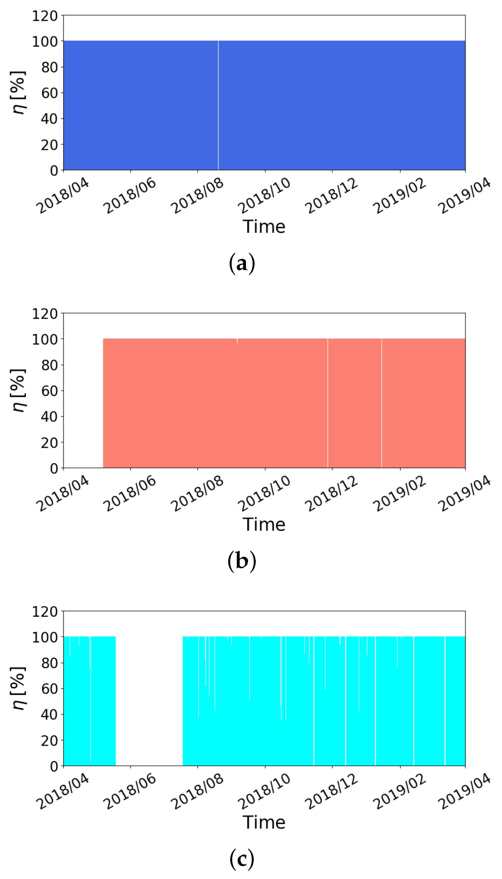
For the cup anemometer, the availability was mostly 100%, though there were occasions with 0% availability. Due to the concentration of the large number of data points in Figure 4a, the time slots with $\eta =0\%$ are not visible. For the sonic anemometer, the data acquisition system at the meteorological mast had trouble and it could not store the measured wind data until the first week of May 2018. Consequently, the availability was 0% for this period. Regarding the LiDAR, it was sent for maintenance from May 18 through July 18 and thus, the availability for this period was 0%. Although $\eta$ was mostly 100% when the LiDAR was operating, there were occasions when the LiDAR was unable to measure the wind speed (i.e., $\eta =0\%$) or the availability $\eta$ was less than 100%. Note that the maximum number of 10-min data that a device can collect in a one-year time period is 52,560. However, in order to collect the maximum number of data, a device has to operate ideally for the entire year, which is not possible, and measurement devices usually collect less data. For example, the number of actually measured 10-min average data for the cup anemometer is 46,970. The availability of this 10-min averaged data (${\eta }_{10}$) can be defined as:

$${\eta }_{10}=\frac{N_{10,\mathrm{meas}}}{N_{10,\max }}\times 100\%$$

(2)

where $N_{10,\mathrm{meas}}$ is the actual number of 10-min average data and $N_{10,\max }$ is the maximum possible number of 10-min average data that can be collected in the given period. This makes the yearly availability of the cup anemometer equal to 89%. The missing data of roughly 10% is difficult to observe in Figure 4a, since a large amount of data from the one year period is concentrated in this figure. Similarly, the yearly availability of the sonic anemometer and the V2 LiDAR are 81% and 75% respectively. It was possible to compare and analyze data from a shorter measurement campaign when all three devices were operating perfectly and were able to collect measurements with $\eta =100\%$. This was done in many earlier studies. However, operational issues and problems are commonplace in field measurements, especially when the measurements are conducted for longer periods. Therefore, the current study also considers those periods when data was not collected by one or more devices.

3.1. Mean Wind Speed and Turbulence Intensity

This section presents the 10-min average wind speed, standard deviation and turbulence intensity measured by the sonic anemometers, the cup anemometers and the profiling LiDAR. The study uses sonic anemometers as reference devices because of their high sampling rate and because they are the preferred device in measurements of atmospheric turbulence [20,23]. As stated earlier, comparisons are conducted using data collected for a period of one year. Furthermore, the minimum threshold of data availability ($\eta$) for the LiDAR and sonic anemometers is set to 80% throughout the study. Experience shows that LiDAR data with lower availability contribute to an increase in uncertainty and to a reduction in the overall data quality.

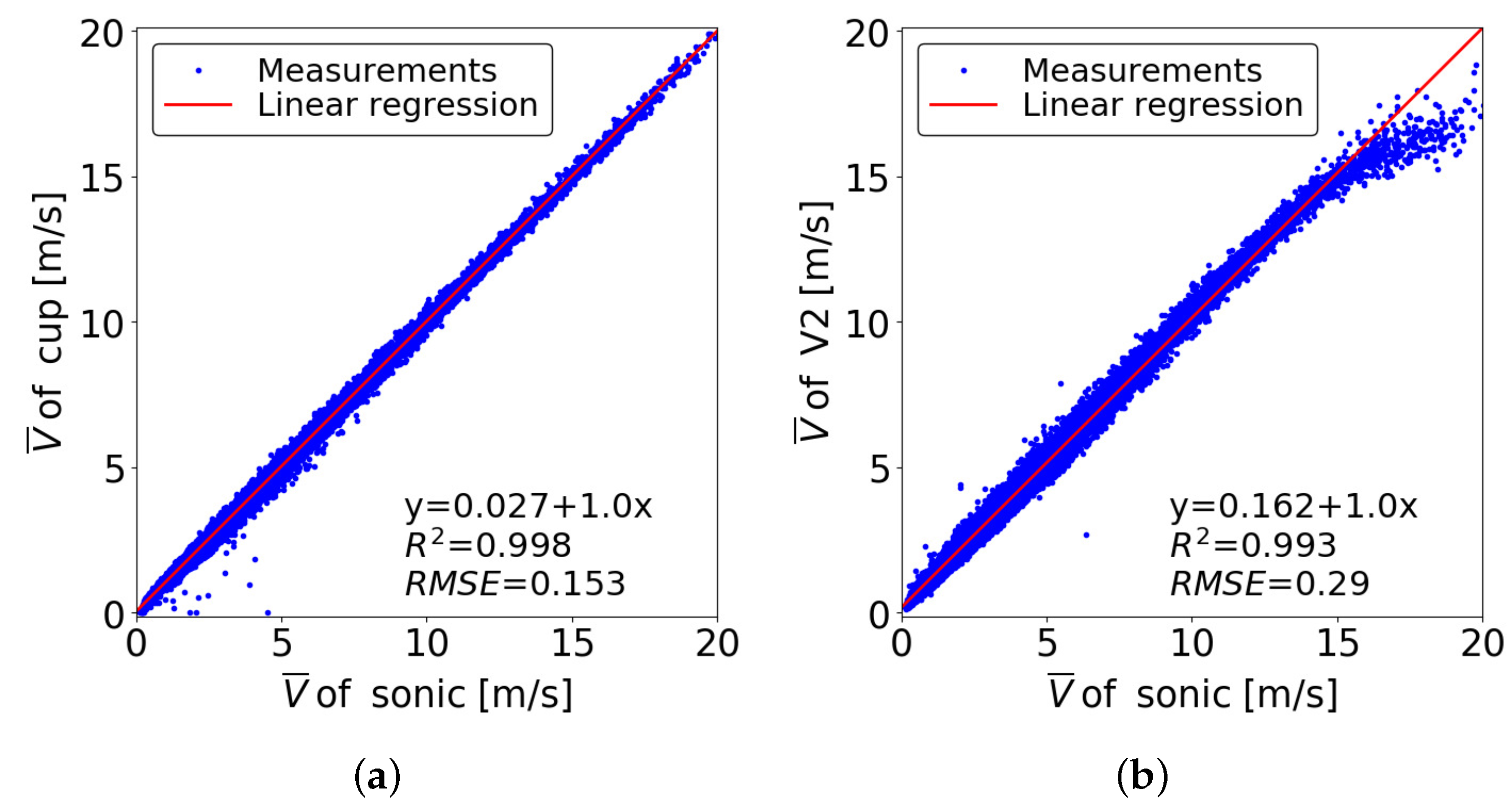
Figure 5 presents a comparison of 10-min averaged horizontal velocities ($\overline{V}$) measured by the cup anemometer and the V2 LiDAR against measurements collected by the sonic anemometer at 40 m height. Here, $\overline{V}$ is defined by

$$\overline{V}=\frac{1}{T}{\int }_t^{t+T}V(t)dt=\frac{1}{N_T}\sum _{i=N_t}^{N_{t+T}}{V}_i,$$

(3)

where $V(t)$ and $V_i$ are the instantaneous horizontal velocity in the continuous and discrete form, T is the average time period (10 min in this study), and $N_T$ is the total number of data in the 10-min time period. While the cup anemometer directly measures $V_i$, for the sonic anemometer and the LiDAR, $V_i$ is computed using $V_i=\sqrt{(u_i^2+v_i^2)}$, where $u_i$ and $v_i$ are wind speed components in the west to east and south to north directions, respectively. Comparison between the cup and sonic anemometers in Figure 5a shows good agreement. The regression line obtained from linear least squares fitting indicates the uncertainties in the comparison. The slope of the line is 1.0, while the offset is 0.022 m/s. Coefficient of determination $R^2$ of 0.998 can be considered to be significantly high. There are a few outliers for lower wind speeds, i.e., when $\overline{V}$ from the sonic anemometer is less than 5 m/s. This may be due to the fact that uncertainties in the cup anemometer measurement is higher for lower wind speeds. Nevertheless, even at lower wind speeds, the overall agreement between the cup anemometer and the sonic anemometer is fairly good. Note that the number of data pairs used for this comparison is 40375. Comparison between the V2 LiDAR and the sonic anemometer in Figure 5b shows a larger variation, although the slope of the regression line is still 1.0 and $R^2$ is 0.993 which is still quite high. Conspicuous differences between the LiDAR and the sonic anemometer measurements can be observed at higher wind speeds, i.e., $\overline{V}$ of the sonic anemometer is larger than 15 m/s. The LiDAR-measured wind speeds are lower at higher wind speeds for this height. One possible reason that was initially considered was that the site experiences high wind speeds predominantly in winter when snowfall is frequent. Because the horizontal speed of snow would usually be lower than the actual wind speed, the laser beam reflected from the snow particles would show a lower wind speed. However, this underestimation in LiDAR measurement is not observed from the comparison of wind speed at 57 m height (cf. Figure 9a). Another source of this discrepancy could be due to interference of the tower wake. However, this would have reduced the wind speed of the sonic anemometer and not the LiDAR. However, the agreement between the LiDAR and the sonic anemometer, with respect to the mean wind speed, is acceptable. The number of data pairs in this comparison is 30,959, which is approximately 10,000 less than for the sonic anemometer and cup anemometer comparison. This is due to the lower data availability of the LiDAR measurement.

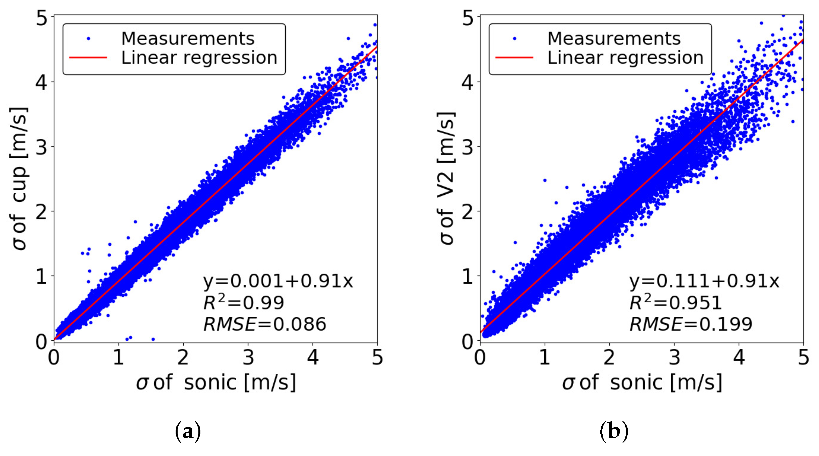
Figure 6 presents a comparison of the standard deviation of the horizontal velocities measured by the cup anemometer and the V2 LiDAR against the measurements collected by the sonic anemometer at 40 m height. The variation in the comparison of the standard deviation is higher than that for the mean wind speed. This larger difference comes from the definition of the standard deviation ($\sigma$), which is the square root of the second central moment of velocity, i.e.,

$$\sigma =\sqrt{\frac{1}{N_T}\sum _{i=N_t}^{N_{t+T}}{(V_i-\overline{V})}^2}=\sqrt{\frac{1}{N_T}\sum _{i=N_t}^{N_{t+T}}{V}_i^2-{\overline{V}}^2}.$$

(4)

The square of the velocity fluctuation in $\sigma$ means the differences between the $\sigma$ measured by the two devices will also be larger compared to the mean wind speed. The slope and offset of the regression line from the cup and sonic anemometers comparison are 0.91 and 0.001 respectively, while $R^2$ is 0.99. As it is clear from Figure 6b, the standard deviation from the LiDAR has a larger variation compared to the sonic anemometer; the slope, offset and $R^2$ are 0.91, 0.107 and 0.952 respectively. The variation in the LiDAR and the sonic anemometer comparison increases with increasing $\sigma$. Earlier studies also showed the same degree of difference or larger difference between LiDAR and conventional wind speed sensors like cup or sonic anemometers (see e.g., Sathe & Mann [14,15]). However, the measurement periods in earlier studies were very short–from a few days to one or two months. It should be noted that statistics related to uncertainty obtained from Linear regression are not very meaningful for a long term comparison. For example, the relation for the regression line indicates that the LiDAR should under-estimate the $\sigma$ values when compared against sonic anemometer measurements larger than 1.19 m/s. However, the distribution is spread over a large band. This may be because of the variety of atmospheric conditions—including the stability—that the site experiences during a long-term comparison as performed in the current study. Thus, the least square fitting or the coefficient of determination are not sufficient to quantify the performance of LiDAR for their long term deployment.

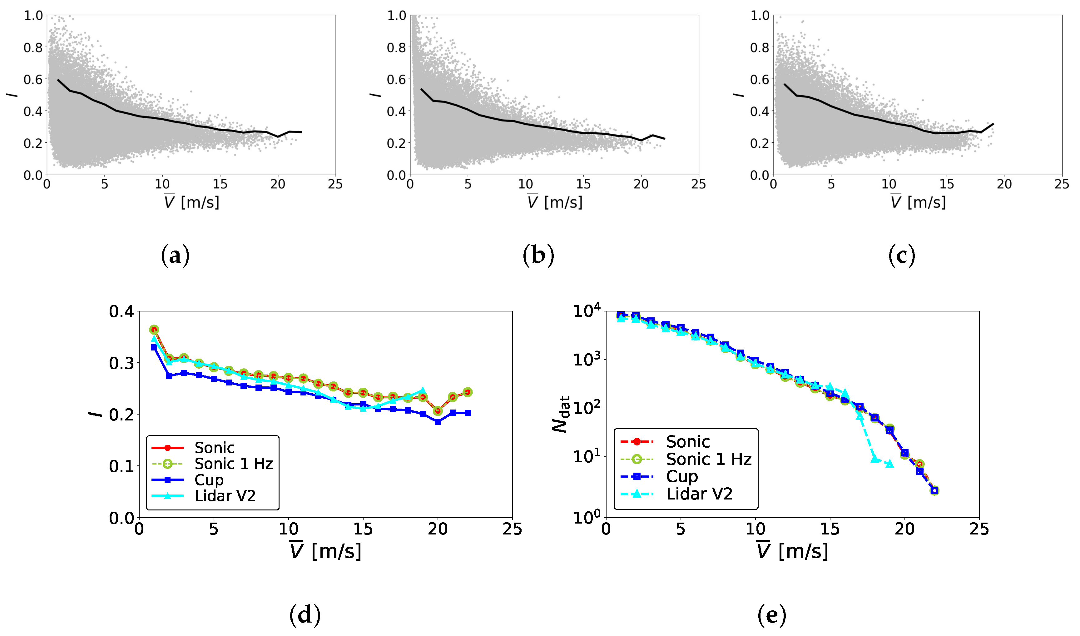
Figure 7 presents the distribution of turbulence intensity as a function of mean wind speed. Turbulence intensity (I) is defined by

$$I=\frac{\sigma }{\overline{V}}.$$

(5)

Measurements from all three instruments show a similar trend; the higher turbulence intensities occur during lower wind speeds and they gradually decrease with increasing mean wind speed. Furthermore, variation of the turbulence intensity is larger when the wind speed is low. Variation is particularly large for the cup anemometer measurements with too many points close to or even larger than $I=1.0$, but it should be noted that the measurements from cup anemometer as well as from LiDAR are not very reliable when the wind speed is low. Regarding the LiDAR, the turbulence intensities are mainly concentrated below $I=0.8$ even at the lowest mean wind speed. Although not presented explicitly in the paper, the 90th percentile line of the LiDAR data shows better agreement than that of the cup anemometer data when compared against the sonic anemometer measurement. Figure 7d shows the bin-averaged turbulence intensities for mean wind speed bins of size 1 m/s, and Figure 7e shows the number of turbulence intensity data per bin. Among the three instruments, the cup anemometer has the lowest turbulence intensity for almost all wind speed bins. The LiDAR-measured turbulence intensities overlap with the sonic anemometer-measured data when the wind speed is low. However, the bin-averaged turbulence intensity of the LiDAR gradually decreases for higher mean wind speeds. This tendency contradicts with a similar comparison by Bot [21], who showed that LiDAR-measured turbulence intensities were usually larger than or similar to the sonic anemometer-measured data. It should be mentioned however, that the maximum number of 10-min data sets per bin in their investigation was between 1000 to 2500, whereas in the current study, the maximum number of data per bin is close to 10,000 and there are more than 1000 data sets in each bin up to 10 m/s (cf. Figure 7e). Nevertheless, neither earlier studies nor the current study can describe the general trend regarding the magnitude of turbulence intensities measured by these three devices. For example, as discussed below, the bin-averaged turbulence intensities at a higher altitude of 57 m are larger for the LiDAR than for the sonic anemometer for most of the mean wind speed range (cf. Figure 10). The turbulence intensities measured by these three devices depend on the altitude, terrain as well as atmospheric conditions. One thing that can be stated with certainty is that LiDAR-measured turbulence intensity shows better agreement with sonic anemometer data than does cup anemometer data. As a result, the fatigue load that a wind turbine may experience, computed using LiDAR-measured turbulence intensity, will be more reliable than that estimated using cup anemometer measurements. The lower turbulence levels measured by a cup anemometer are attributed to the longer response time related to its inertia arising from the moving components such as cups and horizontal arms [29].

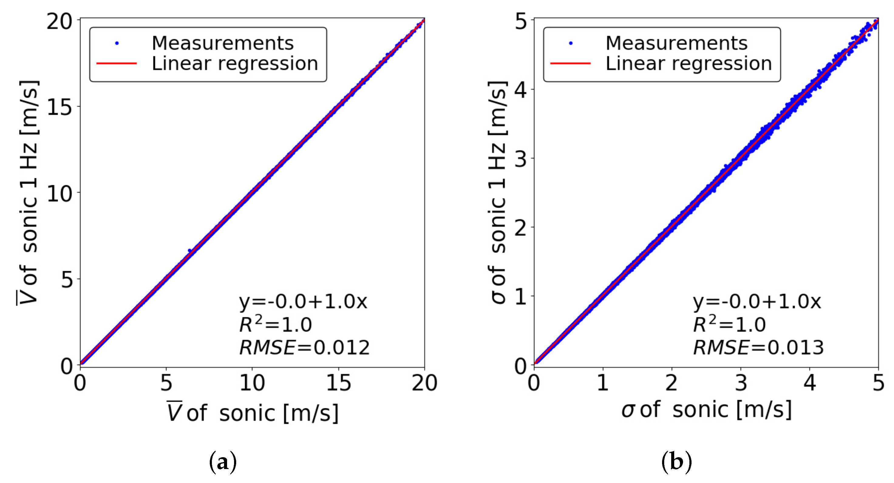
One major concern with the use of LiDARs in wind energy applications is their low sampling frequency. The V2 profiling LiDAR deployed in the current study collects wind data at 1 Hz sampling frequency compared to the 10 Hz sampling frequency of sonic anemometers (cf. Table 1). Considering that the lower sampling rate (of both the LiDAR and the cup anemometer) may filter out small-scale turbulence structures, Figure 8 compares the original 10 Hz sonic anemometer data against the sonic anemometer data re-sampled at 1 Hz. As is clear from both the mean wind speed and standard deviation, the difference between the 10 Hz and 1 Hz data is negligible. As a reference, the distribution of the turbulence intensity using this re-sampled sonic anemometer data is also plotted in Figure 7d. The 1 Hz data overlaps with the original sonic anemometer data. This suggests that turbulence structures with time scales smaller than one second have negligible contribution to the total turbulence kinetic energy and therefore can be ignored for atmospheric boundary layer (ABL) turbulence. A sampling frequency of 1 Hz is sufficient for wind resource assessment and characterization of the site turbulence.

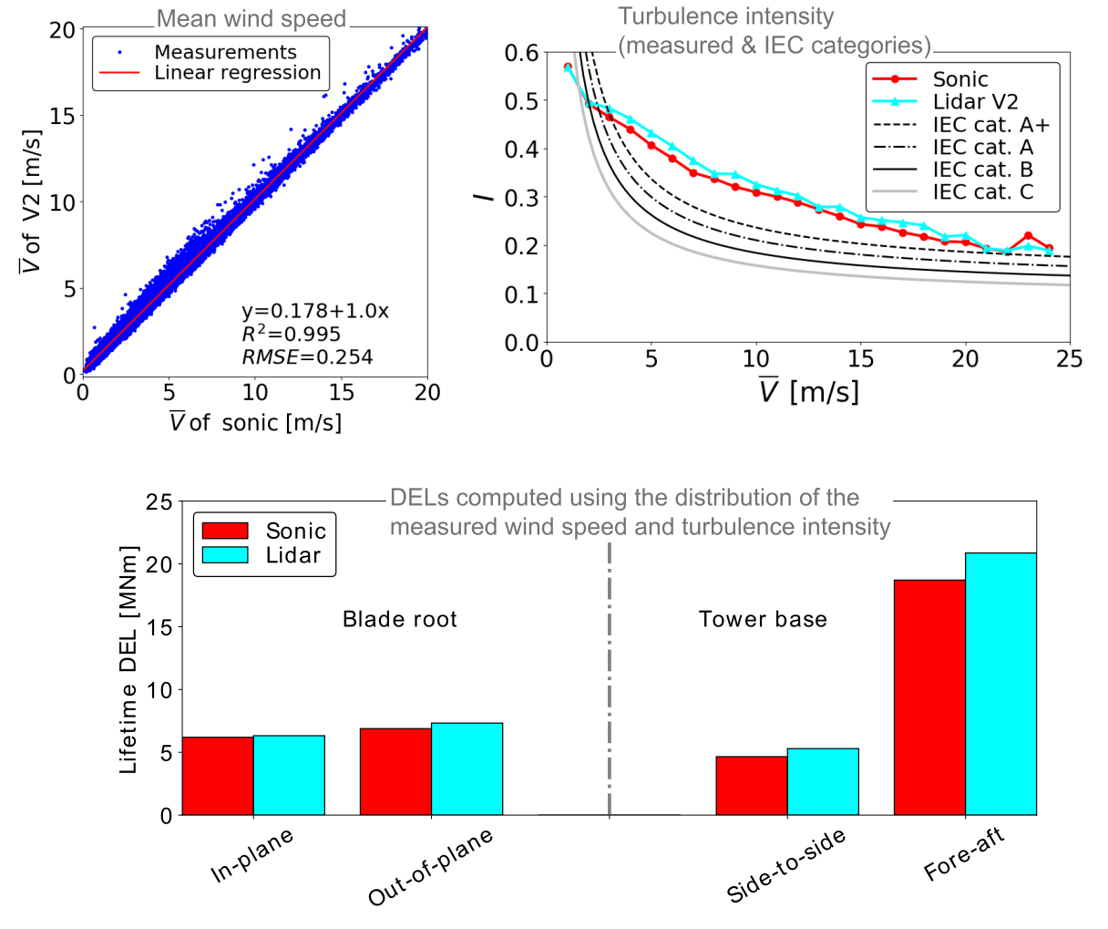
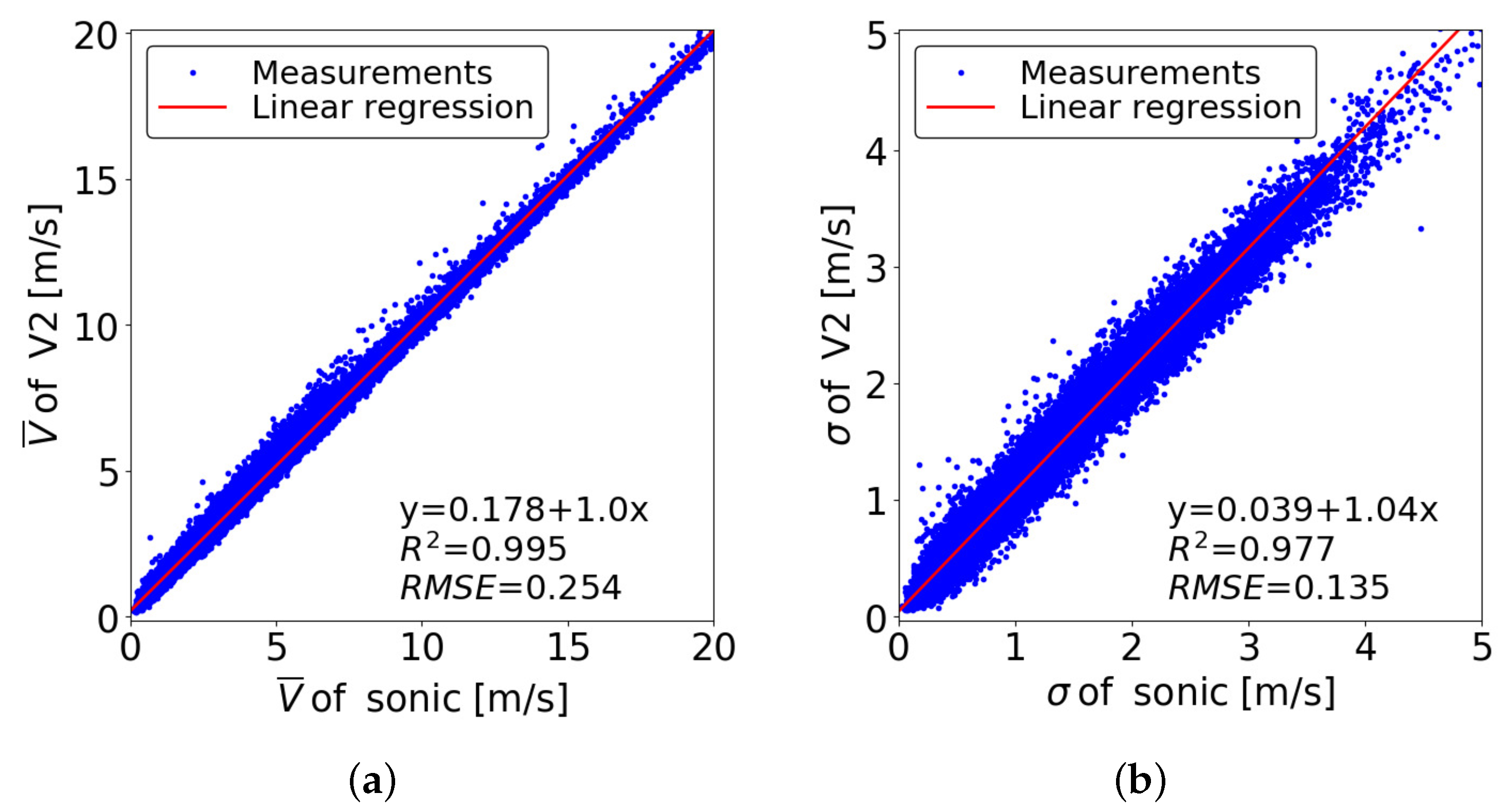
Figure 9 compares the LiDAR-measured mean wind speed and standard deviation against the measured data from the sonic anemometer installed at 57 m height. This is the highest point on the tower where a sensor is installed and disturbance of the wind due to the tower is negligible at this height. The mean wind speeds from the LiDAR show good agreement with those measured by the sonic anemometer, with the slope and offset of the regression line being 1.0 and 0.178 while $R^2=0.995$. Furthermore, underestimation of higher mean wind speeds by the LiDAR, which was observed at 40 m height, disappears at this height. The uncertainty in $\sigma$ measured by the LiDAR decreases at 57 m height; the slope, offset and $R^2$ are 1.04, 0.039 and 0.977 respectively. The DBS method employed by the profiling LiDAR assumes horizontal homogeneity at the measurement height. However, the distance between the four measurement points increases with increasing height, and as a consequence, horizontal homogeneity may not be satisfied. The effect should be more pronounced for the standard deviation measurement. Despite this inherent characteristic of the DBS method, it is interesting to observe that the agreement between the LiDAR and the sonic anemometer measurements is better at 57 m. The number of data pairs used in this comparison is 34,783.

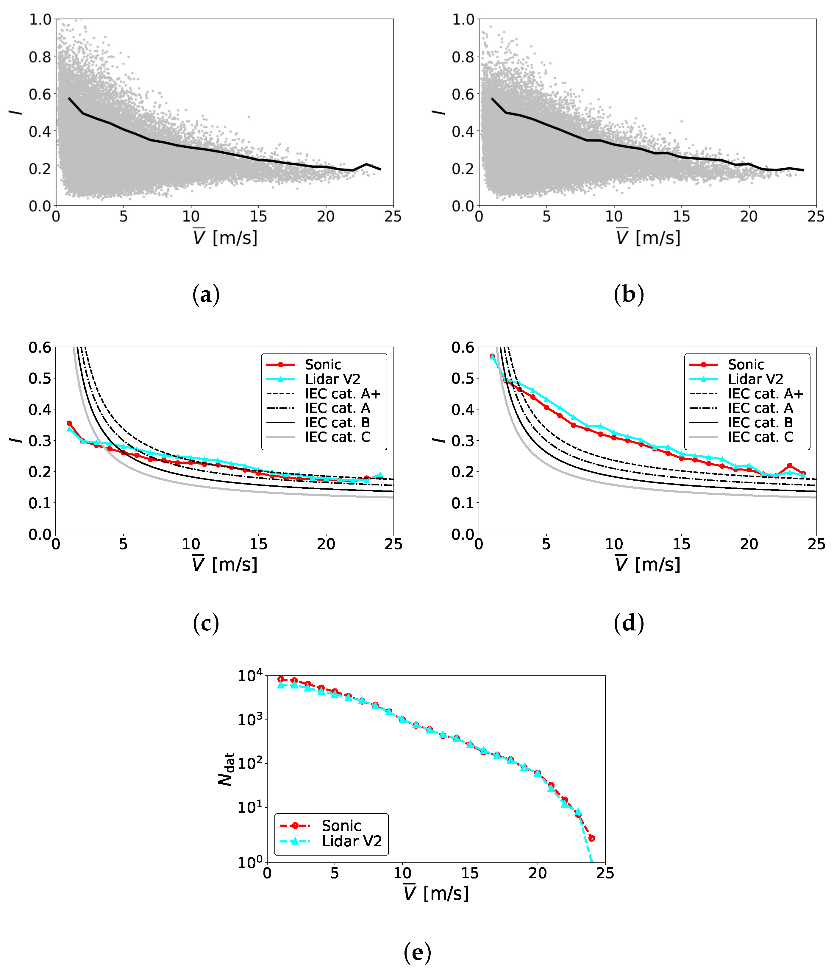
Figure 10 presents the distribution of turbulence intensity as a function of mean wind speed at 57 m height. The tendencies are similar to those at 40 m height. The bin-averaged turbulence intensity for the LiDAR is higher than that from the sonic anemometer for the mean wind speed range of 2 to 20 m/s. For reference, turbulence categories for the wind turbine classes defined in the IEC standard [30] are also included in the figure. These standard turbulence intensity values are defined as:

$$I_{\mathrm{IEC}}=\frac{I_{\mathrm{ref}}(0.75{\overline{V}}_{\mathrm{h}}+b)}{{\overline{V}}_{\mathrm{h}}},$$

(6)

where $I_{\mathrm{ref}}$ is the reference value of the turbulence intensity, ${\overline{V}}_{\mathrm{h}}$ is the hub height wind speed and $b=5.6$ m/s. The IEC standard has four categories of reference turbulence intensities—A+ ($I_{\mathrm{ref}}=0.18$), A ($I_{\mathrm{ref}}=0.16$), B ($I_{\mathrm{ref}}=0.14$) and C ($I_{\mathrm{ref}}=0.12$)—for defining wind turbine classes. Note that for class S, the turbulence intensity and other parameters are specified by the designer [30]. The bin-averaged turbulence intensity values measured by both the sonic anemometer and the LiDAR are less than or similar to the turbulence intensity for category A+. For $\overline{V}\le 6$ m/s, the measured values are even lower than category A, although for $10\le \overline{V}\le 15$ m/s, the LiDAR-measured bin-averaged values are slightly larger than category A+. However, the IEC standard specifies that for the normal turbulence model (NTM), the representative value of the standard deviation should be set to the 90th percentile for the given wind speed [30]. This is shown in Figure 10d. For $\overline{V}>3$ m/s, the turbulence intensity values—obtained from the 90th percentile of $\sigma$—measured by both the sonic anemometer and the LiDAR are larger than category A+ of the IEC standard. Thus, both the sonic anemometer and the LiDAR measurements show that the site requires ‘class S’ wind turbines which can withstand the site-specific higher turbulence intensity. It can be appreciated from this figure that the LiDAR-measured turbulence intensities are slightly larger (by about 2% or less) than those measured by the sonic anemometer, although the difference between the two measurement sets is not very significant. The effect of this difference on the wind turbine fatigue load is quantified and discussed in Section 4. Note that all further analyses use measurement data from 57 m height.

3.2. Peak Wind Speed

Peak gust wind speeds are an important parameter for the design of wind turbines or any other structures that experience wind loading. The IEC [30]—the lead organization responsible for the standardization of the wind turbine design process—has several specifications related to gust winds. Although the models for gust defined in the IEC standard or other guidelines for wind turbine certifications (see e.g., the GL Guideline [31]) are simplified models which can be easily implemented in the aeroelastic code for faster simulation, rigorous measurement may be necessary to improve the models or simply to modify them for site-specific conditions. Note that the extreme wind speeds that turbines must be designed to withstand are defined in terms of the recurrence or return period. An extreme wind speed with a recurrence period of $N_{\mathrm{y}}$ years (usually $N_{\mathrm{y}}$ is one year or 50 years) has an annual probability of occurrence of $1/N_y$. Measurement of extreme wind speeds is difficult, since their frequency of occurrence is low. However, it is often a practice to estimate extreme wind speeds from measurements over a shorter period (usually one year) and to use them together with statistical models specified in guidelines to estimate extreme wind speeds with long recurrence periods [29,30]. Therefore, accurate measurement of peak wind speed is still crucial. However, with the instantaneous wind speed being a random process, the peak or gust wind speed for each 10-min window will also become a random variable.

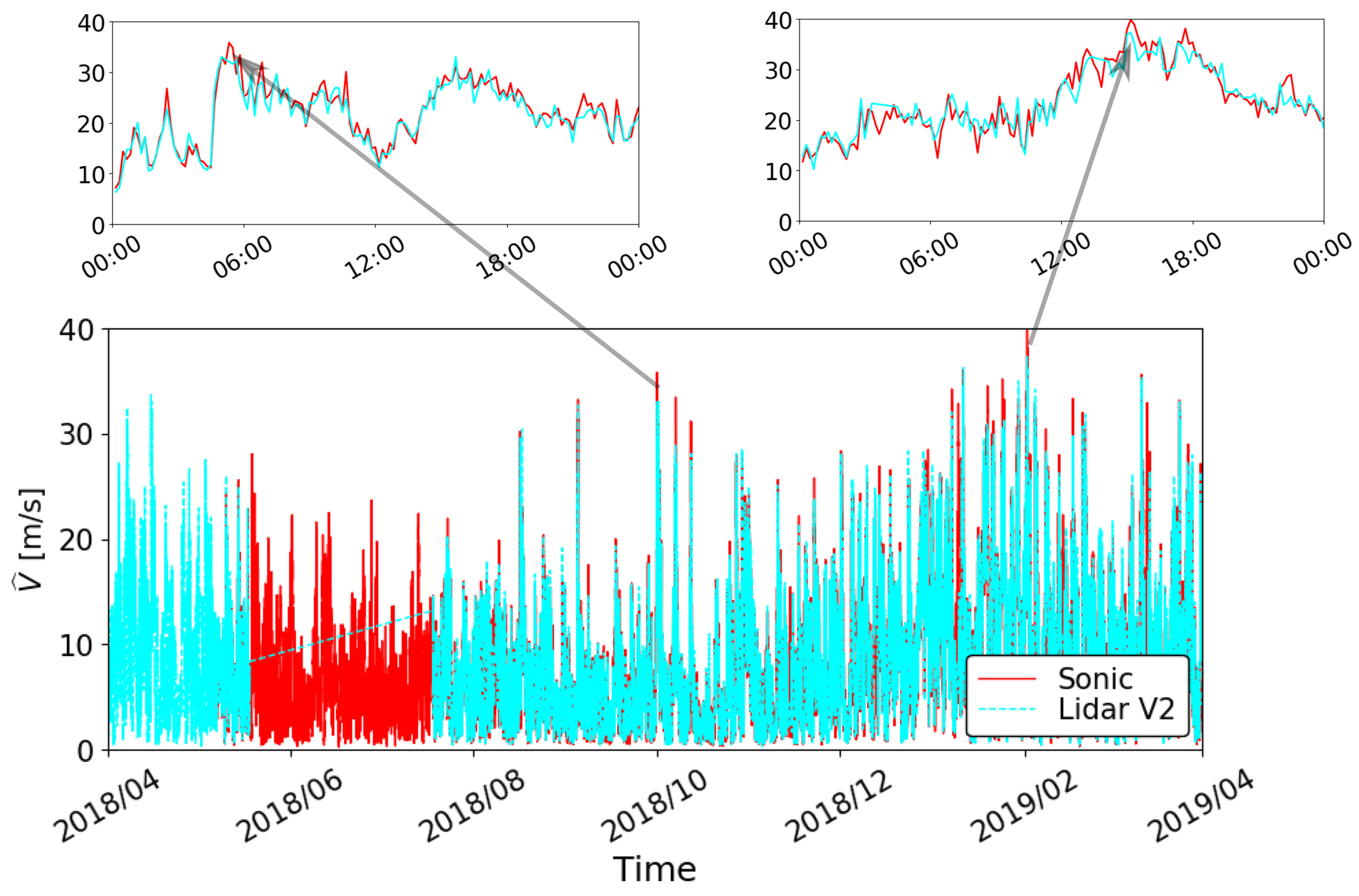
Figure 11 compares the sonic anemometer-measured and LiDAR-measured time series of the peak wind speed ($\widehat{V}$) in every 10-min time window for one-year period and at 57 m height. It can be appreciated that $\widehat{V}$ measured by the sonic anemometer has a larger amplitude compared to that measured by the LiDAR. For example, in the two zoom-in figures, the highest value of the peak wind speed occurs around the same time for both the sonic anemometer and the LiDAR measurements. In the left zoom-in figure, the peak wind speed (pointed by the arrow) measured by the sonic anemometer is 33.3 m/s, while that measured by the LiDAR is 32.3 m/s, i.e., lower by roughly 3% for the LiDAR. Similarly, in the right zoom-in figure, the maximum values of the peak wind speed for the sonic anemometer and the LiDAR are 39.8 m/s and 37.3 m/s respectively, i.e., the LiDAR measurement is 6.3% lower than the sonic anemometer measurement. This is one of the limitations of the LiDAR, and the comparatively lower value of the peak wind speed may be the combined effect of the lower sampling frequency and the characteristics of the DBS mode. However, in wind engineering, it is a common practice to employ a moving average filter with an averaging time of 3 s when evaluating gusts at a site [32].

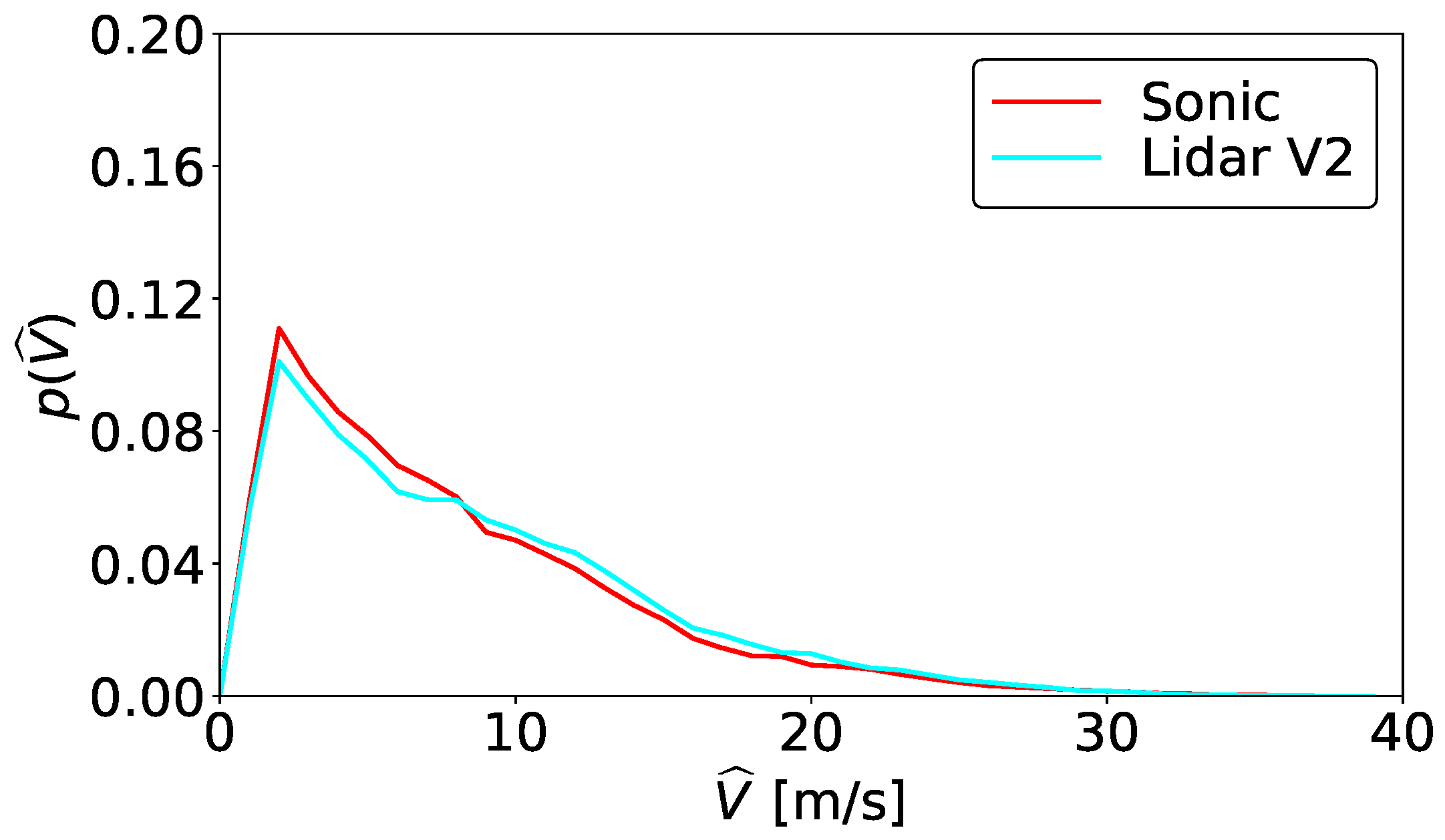
Figure 12 shows the probability density function (PDF) of $\widehat{V}$ obtained from the sonic anemometer and the V2 LiDAR. It is interesting to observe that while for $\widehat{V}<9\mathrm{m}/\mathrm{s}$, the sonic anemometer has higher PDF values, when $\widehat{V}$ is larger than 9 m/s, either the V2 LiDAR has larger PDF value or the values are almost the same for both devices. This indicates that the probability of occurrence of higher $\widehat{V}$ is similar for both the sonic anemometer and the LiDAR. However, this result should be observed with caution, since the number of data sets decreases with increasing $\widehat{V}$ in the current measurement campaign.

In wind engineering, peak wind speed ($\widehat{V}$) is usually expressed as a function of mean wind speed ($\overline{V}$) and turbulence intensity (I):

$$\widehat{V}=\left(1+gI\right)\overline{V}=G\overline{V},$$

(7)

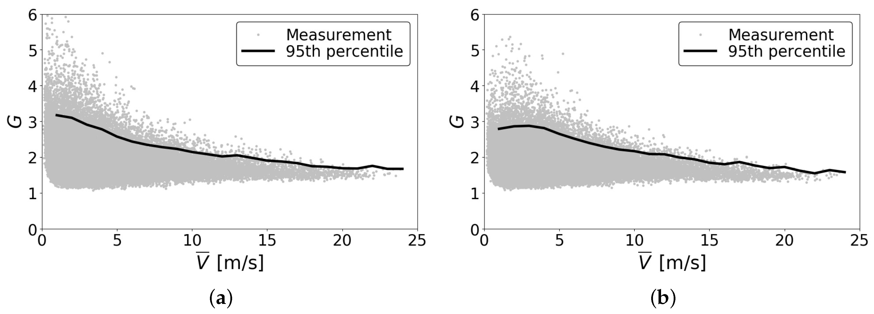
where $g=(\widehat{V}-\overline{V})/\sigma$ is the peak factor and $G=\widehat{V}/\overline{V}$ is the gust factor. Figure 13 shows the distribution of the gust factor as a function of mean wind speed at 57 m height. The 95th percentiles of the measured data are shown by lines in these figures. The gust factor shows a similar trend to the turbulence intensity, i.e., the highest value occurs for the lowest mean wind speed for which the variation is also large. For higher wind speeds, G gradually converges between 1 and 2. For both the sonic anemometer and the profiling LiDAR, G converges roughly to 1.9, i.e., $\widehat{V}$ is 1.9 times $\overline{V}$ during strong wind speeds. One can conclude from these comparisons that LiDAR is able to measure peak wind speeds with a similar accuracy to that of sonic anemometers.

3.3. Effect of Terrain

LiDAR measurements in complex terrain are considered to be prone to larger error and higher uncertainties. The horizontal homogeneity assumption of the DBS technique is not valid in complex terrain which induce inhomogeneity to the local atmospheric boundary layer flow. Past studies used models and computational fluid dynamics (CFD) simulations to correct the error due to complex terrain in the LiDAR measurement [11,33]. However, these and other models are calibrated for the topography of specific sites. As stated earlier, use of multiple LiDARs is also being explored to measure wind speed in complex terrain [34]. This section discusses the accuracy of the classical DBS mode for moderately complex terrain using a long-term measurement campaign.

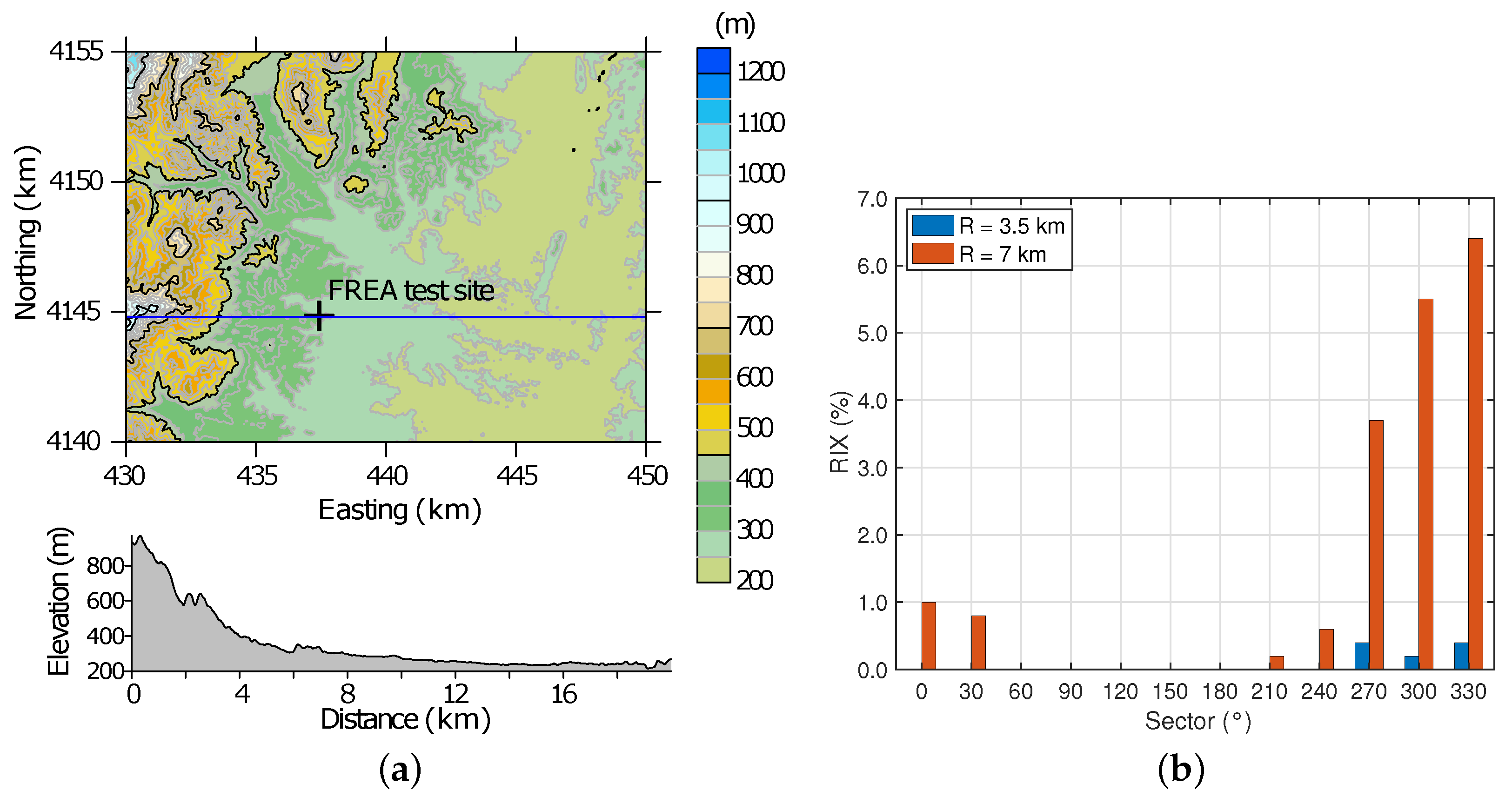
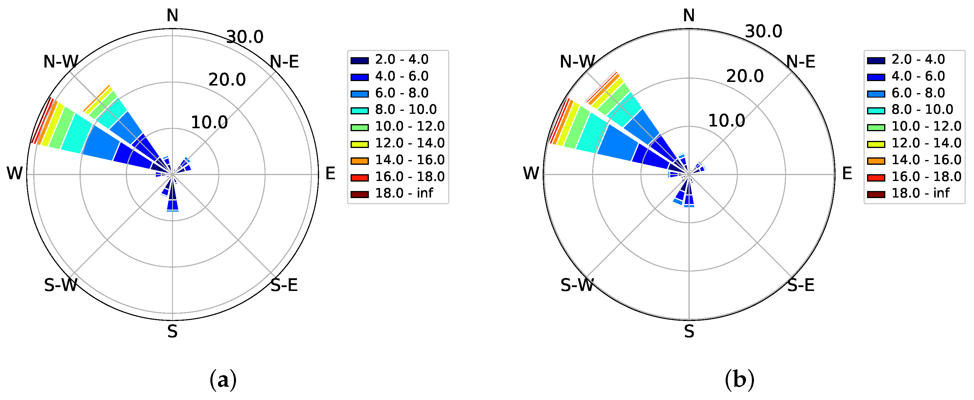
As shown in Figure 2, the ruggedness index of the FREA test site for sector ${60}^{\circ }$ to ${180}^{\circ }$ is almost 0%, i.e., the site is homogeneous for this sector. On the other hand, from ${270}^{\circ }$ through ${330}^{\circ }$, the ruggedness index is 38 to 65%, and thus the wind blowing from this sector should be influenced by moderately complex terrain. Figure 14 shows wind roses from the sonic anemometer measurement and the V2 LiDAR measurement at 57 m height. It can be appreciated that both the sonic anemometer and the LiDAR show a similar distribution of wind speeds and directions. As can be seen in the figures, the dominant wind directions are WNW and NW. All wind speeds above 12 m/s blow from these two directions. However, these directions lie in the sector with moderately complex terrain. The fraction of wind speeds blowing from any other direction is less than 10%.

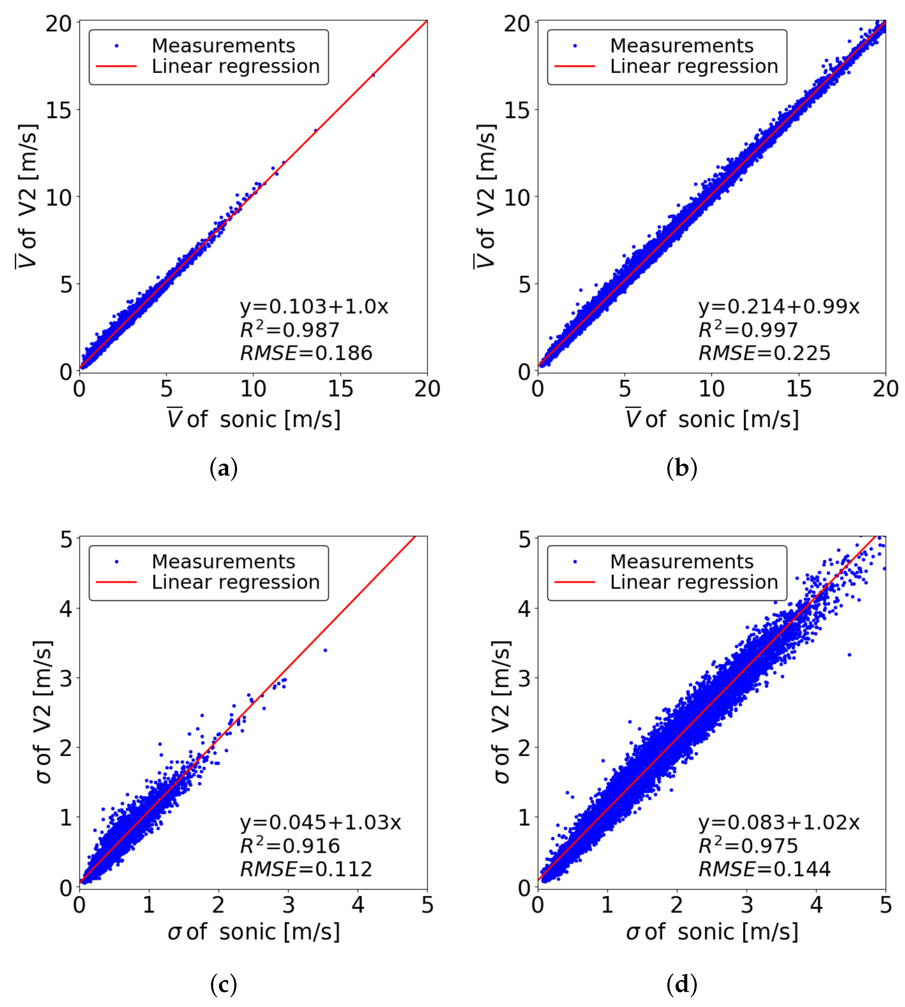
Figure 15 compares the LiDAR measurement for homogeneous terrain (wind direction range ${60}^{\circ }$ to ${180}^{\circ }$) and moderately complex terrain (wind direction range ${270}^{\circ }$ to ${330}^{\circ }$) against the corresponding sonic anemometer data at 57 m height. Note that the number of data for the homogeneous terrain comparison is 4743, while that for the moderately complex terrain comparison is 17,232. For the mean horizontal wind speed, both the homogeneous and complex terrain data sets show good agreement with the sonic anemometer measurement, although the root-mean-square error (RMSE) is higher for the latter. Since the mean wind speeds and number of data sets are lower for the homogeneous case, it is not possible to accurately quantify the comparison. Nevertheless, one can conclude that the LiDAR-measured mean wind speed is accurate for moderately complex terrain. Regarding the standard deviation, $R^2$ is 0.916 for the homogeneous terrain case and 0.975 for the complex terrain case, while the RMSE is 0.112 and 0.144 respectively for the homogeneous and complex terrain cases. The LiDAR performance is roughly the same for both cases. The long-term measurements employed in the current study must have been affected by changing atmospheric stability. For example, even when the wind is blowing from the direction of homogeneous terrain, if the ABL is thermally unstable (i.e., convective ABL), the flow will be non-uniform. Therefore, measured data should be further separated based on the ABL stability. This will be considered in future studies.

4. Wind Resource, Power and Load Comparison

In this section, measured data from the sonic anemometer and that from the profiling LiDAR are used to evaluate the wind resource and wind power potential of the site. The velocity and power distribution obtained from the LiDAR measurement are compared against those obtained from the sonic anemometer measurement. The NREL-5 MW wind turbine is used as a reference to estimate and compare the power production potential of the site. Finally the section compares fatigue load for the NREL-5MW wind turbine estimated using aeroelatic simulations with the wind speed and turbulence intensity distribution of the sonic anemometer and the LiDAR measurements. The aeroelastic simulations were performed using OpenFAST.

Figure 16 summarizes the 10-min average wind speed distribution measured by the sonic anemometer and the profiling LiDAR at 57 m height. Figure 16a shows the distribution of the frequency of occurrence of $\overline{V}$ in each bin with a bin interval of 1 m/s. One can appreciate that both the LiDAR and the sonic anemometer show a similar trend. However, for lower wind speeds ($\overline{V}<5\mathrm{m}/\mathrm{s}$), the frequency of occurrence for the LiDAR measurement is lower than that for the sonic anemometer measurement. In particular, for $\overline{V}=2\mathrm{m}/\mathrm{s}$, the frequency of occurrence for the sonic anemometer is 18% compared to about 16% for the LiDAR. This is possibly because LiDAR measurements are prone to lower carrier-to-noise ratio (CNR) values and larger error when the wind speed is low. Measurements with such low CNR values are filtered out from the current analysis, hence the lower frequency of occurrence for the LiDAR measurement. For higher wind speeds, i.e., $\overline{V}\ge 5\mathrm{m}/\mathrm{s}$, the frequency of occurrence for the LiDAR measurement is slightly higher (higher by less than 1%) than that of the sonic anemometer measurement. These tendencies are also reflected in the Weibull probability density function (PDF) in Figure 16b. The Weibull PDF ($p(\overline{V})$) is given by:

$$p(\overline{V})=\left(\frac{k}{c}\right){\left(\frac{\overline{V}}{c}\right)}^{k-1}\exp \left[-{\left(\frac{\overline{V}}{c}\right)}^k\right],$$

(8)

where k and c are the shape and the scale factors respectively. The Weibull PDFs in the figure are obtained by fitting the above function to the measured data for these two parameters. For the distribution obtained from the sonic anemometer data, $k=1.5$ and $c=4.87$, while for the distribution obtained from the LiDAR data, $k=1.53$ and $c=5.40$. These differences in the Weibull parameters between the sonic anemometer and the profiling LiDAR are not very significant. The annual average wind speed obtained from the sonic anemometer measurement is 4.41 m/s, while that obtained from the LiDAR measurement is 4.79 m/s. Therefore, for the current site, the LiDAR overestimated the wind speed by 0.38 m/s, i.e., by about 8%. Note that the annual wind speed of 4.4 m/s is too low for the site to be considered for wind energy development. A similar long-term comparison study between LiDAR and conventional tower-based measurements at a site with higher wind speeds will help to further evaluate the performance and accuracy of the LiDAR technology.

Next we compare the power production, computed from the measured wind speed. To this end, the power curve of the NREL 5-MW reference wind turbine which has been used extensively in wind energy research [35], is employed. The NREL 5-MW turbine has a rotor diameter and hub height of 126 m and 90 m, respectively. The cut-in, rated and cut-out wind speeds are 3 m/s, 11.4 m/s and 25 m/s. Note however, that the 90 m hub height is higher than the highest measurement point, i.e., 57 m in the current measurement campaign. One way to overcome this issue can be to extrapolate the wind speed at 90 m height using the power law, i.e.

$$\frac{\overline{V}(z)}{\overline{V}(z_{\mathrm{ref}})}={\left(\frac{z}{z_{\mathrm{ref}}}\right)}^{\alpha },$$

(9)

where $\overline{V}(z)$ is the mean wind speed at height z which in this specific case is 90 m, ${\overline{V}}_{\mathrm{ref}}$ is the mean wind speed at height $z_{\mathrm{ref}}$ which is 57 m, and $\alpha$ is the power law exponent. To apply the power law in the current study, we still need to decide a value for $\alpha$. The study showed that $\alpha$ is a highly variable parameter, depending on the nature of the terrain, the atmospheric stability and other thermal and mechanical parameters [36]. It is possible to determine the value of $\alpha$ by fitting Equation (9) to the measured wind data, but an $\alpha$ value obtained in such a way can only be verified against the LiDAR measurement, since the highest measurement point on the meteorological mast is at 57 m. To maintain the reliability of the comparison between the sonic anemometer and the LiDAR measurement, we therefore use the wind speed at 57 m height directly to estimate the power output for the wind turbine. Figure 17a compares histograms of the frequency of occurrence of power values estimated from the sonic anemometer and the LiDAR. Except for those times when the wind turbine is not in the power production mode, i.e., below the cut-in wind speed or above the cut-out wind speed, the LiDAR-measured wind speed produce slightly higher occurrence frequencies. Nevertheless, the power output obtained from both the sonic anemometer and the LiDAR show a similar tendency, and the difference in occurrence frequency between the two devices is less than 1% for all power production bins. The capacity factor estimated from the sonic anemometer-measured wind speed is 15%, and that obtained from the LiDAR-measured wind speed is 17%. The higher capacity factor estimated from the LiDAR measurement can be attributed to the fact that the LiDAR was not able to collect the same fraction of lower wind speed data (which corresponded to those below the cut-in wind speed) as that collected by the sonic anemometer. This resulted in a comparatively smaller duration of the ‘no power production’ mode and consequently in the higher capacity factor from the LiDAR measurement. Figure 17b compares the power duration curves which essentially show the number of hours in the measurement period (usually one year) for which the wind power and the power output of the given turbine are equal to or higher than each particular value. The available wind power values are also obtained for the swept area of the NREL 5-MW turbine. The Power duration curves obtained from the LiDAR-measured wind speed show a high level of agreement with those obtained from the sonic anemometer measurement. The corresponding curves for the two devices almost overlap with each other. Note that the sonic anemometer measurement data extends to 7841 h compared to only 6666 h for the LiDAR. This is because the number of 10-min average wind speed data for the former is 47,046, while that for the latter is only 39,996. However, most of the extra data from the sonic anemometer was measured during lower wind speeds which were below the cut-in wind speed for the reference turbine, and consequently they have minimum effect on the overall power output estimation.

As presented in Figure 10, the LiDAR-measured turbulence intensities are larger than those measured by the sonic anemometer. To quantify the effect of this difference on wind turbine fatigue load estimation, we perform aeroelastic simulations of the NREL 5-MW wind turbine subjected to inflow turbulence corresponding to the sonic anemometer and LiDAR measurements. The simulations are performed using OpenFAST, an open-source aero-hydro-servo-elastic wind turbine simulation tool developed by NREL [25]. The inflow turbulent flow field required by OpenFAST is generated using TurbSim [37]. The simulations are carried out for 12 sets of wind speeds (between 3 and 24 m/s) and turbulence intensities, each for the sonic anemometer and the LiDAR. To this end, the turbulence intensity for each wind speed is set to the values measured by the sonic anemometer and the LiDAR (cf. Figure 10). The simulation results are processed for fatigue load analysis using MLife [38].

Table 2. Details of the simulations for the fatigue load analysis.

Tool	Description	Set-Up and Parameters
		Wind speed: 3–23 m/s at wind step of 2 m/s,
	General input	24 m/s
		Total number of cases: $2\times 12=24$
		Wind type: NTM
		Turbulence model: Kaimal
TurbSim	Turbulent wind field generation	Number of grid points (Vertical × Horizontal): $31\times 31$
		Grid height × Grid width: 145 m × 145 m
		Different random seed used for each simulation
OpenFAST	Aero-servo-elastic simulation	Simulation time (T): 630 s
	of a wind turbine	Discard first 30 s of data
		Time step ($dt$): 0.005 s
		Equivalent load frequency: 1 Hz
MLife	Fatigue load analysis	Number of equivalent cycles: $2.98\times {10}^8$
		Analysis corresponds to 20 year lifetime

describes the simulation cases and major parameters. These analyses essentially correspond to design load case (DLC) 1.2 in the IEC standard [30], which requires fatigue analysis during normal power production mode, with a normal turbulence model and wind speeds between the cut-in and the cut-out speeds. Note that we have not considered yaw misalignment or multiple random seeds for generating turbulent wind field.

Figure 18 shows the damage equivalent loads (DELs) for the blade root and the tower base bending moment obtained from the simulations. DEL is widely used approach for evaluating overall fatigue damage that a wind turbine may experience for the given wind speed and turbulence distribution. The distribution of DELs for the 10-min time-history of loads as a function of mean wind speed are shown in Figure 18a,b. The DEL of the blade root in-plane bending moment and out-of plane bending moment for the sonic anemometer and the LiDAR are close. Only for $\overline{V}=7$ m/s, the out-of-plane bending moment is about 22% lower for the LiDAR. Similarly, the DEL of the tower base bending moment for the sonic anemometer and the LiDAR also show similar tendency. The differences are larger for the fore-aft bending moment, with the largest difference at $\overline{V}=17$ m/s where the DEL for the LiDAR measurements is 21% larger than that for the sonic anemometer measurements. Comparison of the lifetime DELs (20 years) is shown in Figure 18c. The lifetime DELs are computed using the Weibull wind speed distributions for both the devices (cf. Figure 16). Agreement of the lifetime DEL for the blade root bending moments is good for the sonic anemometer and the LiDAR wind field distributions. The LiDAR wind speed overestimate the in-plane and out-of-plane lifetime DEL by 2% and 6% respectively. However, for the tower base moment, the differences are slightly larger. When the LiDAR wind speed distribution is used, side-to-side and fore-aft lifetime DELs are overestimated by about 13% and 11% respectively. However, the difference may also be because of performing only one simulation for each wind speed. It is recommended to perform around six simulations for each wind speed with varying random seeds for generating wind flow fields, and then to take the ensemble of those simulations.

5. Conclusions

The current paper presented the results from a year-long Doppler LiDAR-based measurement campaign with the primary goal of providing an answer to the question of whether a single LiDAR can replace the meteorological tower for wind energy applications. Wind data measured by a profiling LiDAR was compared against those measured using sonic and cup anemometers mounted to a neighboring meteorological mast.

LiDAR-measured wind speeds showed very good agreement with those measured using the sonic anemometer, though the variation in the comparison of the standard deviations was higher than that for the mean wind speeds. The bin-averaged turbulence intensities showed that compared to the cup anemometers, the LiDAR-measured turbulence intensity was closer to the sonic anemometers measurements. Thus, the fatigue load computed using the LiDAR-measured turbulence will be more reliable than that computed using the turbulence measured by the cup anemometers. Furthermore, the gust factor obtained from the sonic anemometer-measured and LiDAR-measured peak wind speed roughly converged to 1.9 showing that the LiDAR is able to measure peak wind speeds with acceptable accuracy (at least up to 57 m height considered in this study). To investigate the applicability of LiDAR in moderately complex terrain, the measurements were divided into those blowing from the homogeneous terrain sector and those blowing from the complex terrain sector. When compared against the sonic anemometer measurements, both the homogeneous and complex terrain data sets showed good agreement. Thus, it can be concluded that—even with the classical DBS mode of measurement—LiDAR-measured wind speeds can be considered to be accurate for moderately complex terrain.

Comparison of the velocity distribution showed that for lower wind speeds ($\overline{V}<5$ m/s), the frequency of occurrence for the LiDAR measurement was lower than that for the sonic anemometer, although for $\overline{V}\ge 5$, the LiDAR measurement showed a slightly higher frequency of occurrence. The difference in the occurrence frequency of power distribution between the two devices for all power production bins was less than 1%. Finally, fatigue loads for wind speed and turbulence distributions for the two devices were assessed in the form of DELs. It was found that the LiDAR measurement overestimated the lifetime DEL by 2%–6% for the blade root bending moments and by 11%–13% for the tower base bending moments.

This study shows that even with the inherently lower data availability and some shortcomings of the classical DBS technique, profiling LiDAR can measure wind speed and turbulence intensity with acceptable accuracy and, therefore, can be deployed for actual wind energy applications. The long-term measurement campaign conducted in this study shows that such measurements can be influenced by a lot of parameters which were not considered in the current study. In future studies, atmospheric stability and other environmental conditions such as snow and rain should also be considered. In addition, measurements at sites with different degrees of complexity and offshore sites will also be important.

References

1. Kelley, N.D.; Jonkman, B.J.; Scott, G.N. Comparing Pulse Doppler LIDAR with SODAR and Direct Measurements for Wind Assessment. In Proceedings of the AWEA2007 Conference and Exhibition, Los Angeles, CA, USA, 3–7 June 2007; p. 20. [Google Scholar]
2. Scholbrock, A.; Fleming, P.; Schlipf, D.; Wright, A.; Johnson, K.; Wang, N. Lidar-Enhanced Wind Turbine Control: Past, Present, and Future. In Proceedings of the American Control Conference (ACC), Boston, MA, USA, 6–8 July 2016; pp. 1399–1406. [Google Scholar]
3. IEA Wind Workshop on Lidar Measurements for Wake Assessment and Comparison with Wake Models; Technical University of Munich: Munich, Germany, 2016.
4. El-Asha, S.; Zhan, L.; Iungo, G.V. Quantification of power losses due to wind turbine wake interactions through SCADA, meteorological and wind LiDAR data. Wind Energy 2017, 20, 1823–1839. [Google Scholar] [CrossRef]
5. Easterbrook, C.C. Estimating Horizontal Wind Fields by Two-dimensional Curve Fitting of Single Doppler Radar Measurements. In Proceedings of the Radar Meteorology Conference, Houston, TX, USA, 22–24 April 1975. [Google Scholar]
6. Koscielny, A.J.; Doviak, R.J.; Rabin, R. Statistical considerations in the estimation of divergence from single-Doppler radar and application to prestorm boundary-layer observations. J. Appl. Meteorol. 1982, 21, 197–210. [Google Scholar] [CrossRef]
7. Krishnamurthy, R. Wind Farm Characterization and Control using Coherent Doppler Lidar. Ph.D. Thesis, Arizona State University, Tempe, Arizona, 2013. [Google Scholar]
8. Smith, D.A.; Harris, M.; Coffey, A.S.; Mikkelsen, T.; Jørgensen, H.E.; Mann, J.; Danielian, R. Wind Lidar Evaluation at the Danish Wind Test Site in Høvsøre. Wind Energy 2006, 9, 87–93. [Google Scholar] [CrossRef]
9. Sathe, A.; Mann, J.; Gottschall, J.; Courtney, M.S. Can wind lidars measure turbulence? J. Atmos. Ocean. Technol. 2011, 28, 853–868. [Google Scholar] [CrossRef]
10. Gottschall, J.; Courtney, M. Verification Test for Three WindCube WLS7 LiDARs at the Høvsøre Test Site; Tech. Rep. Risø-R-1732; Technical University of Denmark: Roskilde, Denmark, 2010. [Google Scholar]
11. Klaas, T.; Pauscher, L.; Callies, D. LiDAR-mast deviations in complex terrain and their simulation using CFD. Met. Z. 2015, 24, 591–603. [Google Scholar] [CrossRef]
12. Barthelmie, R.J.; Wang, H.; Doubrawa, P.; Pryor, S.C. Best Practice for Measuring Wind Speeds and Turbulence Offshore through In-Situ and Remote Sensing Technologies; Report to the Department of Energy as Partial Fulfilment of Grant EE0005379; Cornell University: Ithaca, NY, USA, 2016. [Google Scholar]
13. Shimada, S.; Takeyama, Y.; Kogaki, T.; Ohsawa, T.; Nakamura, S. Investigation of the Fetch Effect Using Onshore and Offshore Vertical LiDAR Devices. Remote Sens. 2018, 10, 1408. [Google Scholar] [CrossRef]
14. Sathe, A.; Mann, J. A review of turbulence measurements using ground-based wind lidars. Atmos. Meas. Tech. 2013, 6, 3147–3167. [Google Scholar] [CrossRef] [Green Version]
15. Sathe, A.; Banta, R.M.; Pauscher, L.; Vogstad, K.; Schlipf, D.; Wylie, S. Estimating Turbulence Statistics and Parameters from Ground- and Nacelle-Based Lidar Measurements IEA Wind Task 32; DTU Wind Energy: Roskilde, Denmark, 2015. [Google Scholar]
16. Wilson, D.A. Doppler Radar Studies of Boundary Layer Wind Profiles and Turbulence in Snow Conditions. In Proceedings of the 14th Conference on Radar Meteorology, Tuscon, AZ, USA, 17–20 November 1970; pp. 191–196. [Google Scholar]
17. Kropfli, R.A. Single Doppler radar measurements of turbulence profiles in the convective boundary layer. J. Atmos. Ocean. Technol. 1986, 3, 305–314. [Google Scholar] [CrossRef]
18. Eberhard, W.L.; Cupp, R.E.; Healy, K.R. Doppler Lidar Measurement of Profiles of Turbulence and Momentum Flux. J. Atmos. Ocean. Technol. 1989, 6, 809–819. [Google Scholar] [CrossRef] [Green Version]
19. Sjöholm, M.; Mikkelsen, T.; Mann, J.; Enevoldsen, K.; Courtney, M. Spatial Averaging-effects on Turbulence Measured by a Continuous-wave Coherent Lidar. Met. Z. 2009, 18, 281–287. [Google Scholar] [CrossRef]
20. Mann, J.; Peña, A.; Bingöl, F.; Wagner, R.; Courtney, M.S. Lidar Scanning of Momentum Flux in and above the Atmospheric Surface Layer. J. Atmos. Ocean. Technol. 2010, 27, 959–976. [Google Scholar] [CrossRef]
21. Bot, E.T.G. Turbulence Assessment with Ground Based LiDARs; Tech. Rep. ECN-E–14-043; ECN: Petten, The Netherlands, 2014. [Google Scholar]
22. Mann, J.; Cariou, J.P.; Courtney, M.S.; Parmentier, R.; Mikkelsen, T.; Wagner, R.; Lindelöw, P.; Sjöholm, M.; Enevoldsen, K. Comparison of 3D Turbulence Measurements using Three Staring Wind LiDARs and a Sonic Anemometer. Met. Z. 2009, 18, 135–140. [Google Scholar] [CrossRef]
23. Fuertes, F.C.; Iungo, G.V.; Porte-Agel, F. 3D Turbulence Measurements using Three Synchronous Wind LiDARs: Validation against Sonic Anemometry. J. Atmos. Ocean. Technol. 2014, 31, 1549–1556. [Google Scholar] [CrossRef]
24. Newman, J.F.; Bonin, T.A.; Klein, P.M.; Sonia, W.; Newsom, R.K. Testing and Validation of Multi-LiDAR Scanning Strategies for Wind Energy Applications. Wind Energy 2016, 19, 2239–2254. [Google Scholar] [CrossRef]
25. NREL: OpenFAST. Available online: https://nwtc.nrel.gov/OpenFAST (accessed on 15 July 2019).
26. Land Processes Distributed Active Archive Center. Available online: https://lpdaac.usgs.gov/citing_our_data (accessed on 8 March 2019).
27. Mortensen, N.G.; Bowen, A.J.; Antoniou, I. Improving WAsP Predictions in (too) Complex Terrain. In Proceedings of the European Wind Energy Conference and Exhibition (EWEC), Athens, Greece, 27 February–2 March 2006. [Google Scholar]
28. IEC 61400-12-1 Wind Energy Generation Systems—Part 12-1: Power Performance Measurements of Electricity Producing Wind Turbines, 2nd ed.; IEC Central Office: Geneva, Switzerland, 2017.
29. Manwell, J.F.; McGowan, J.G.; Rogers, A.L. Wind Energy Explained: Theory, Design and Application; John Wiley & Sons: West Sussex, UK, 2009. [Google Scholar]
30. IEC 61400-1 Wind Energy Generation Systems—Part 1: Design Requirements, 4th ed.; IEC Central Office: Geneva, Switzerland, 2019.
31. Guideline for the Certification of Wind Turbines; Germanischer Lloyd: Hamburg, Germany, 2010.
32. Holmes, J.D. Wind Loading of Structures, 3rd ed.; CRC Presee Taylor & Francis Group: Boca Raton, FL, USA, 2009. [Google Scholar]
33. Bingöl, F.; Mann, J.; Foussekis, D. Modeling Conically Scanning LiDAR Error in Complex Terrain with WAsP Engineering; Tech. Rep. Risø-R-166; Technical University of Denmark: Roskilde, Denmark, 2008. [Google Scholar]
34. Pauscher, L.; Vasiljevic, N.; Callies, D.; Lea, G.; Mann, J.; Klaas, T.; Hieronimus, J.; Gottschall, J.; Schwesig, A.; Kühn, M.; et al. An Inter-comparison Study of Multi- and DBS LiDAR Measurements in Complex Terrain. Remote Sens. 2016, 8, 782. [Google Scholar] [CrossRef]
35. Jonkman, J.; Butterfield, S.; Musial, W.; Scott, G. Definition of a 5-MW Reference Wind Turbine for Offshore System Development; Tech. Rep. NREL/TP-500-38060; National Renewable Energy Laboratory: Boulevard, CO, USA, 2009.
36. Gryning, S.E.; van Ulden, P.; Larsen, R.E. Dispersion from a Continuous Ground-level Source Investigated by a K model. Quat. J. R. Met. Soc. 1983, 109, 355–364. [Google Scholar] [CrossRef]
37. Kelley, N.D.; Jonkman, B.J. Overview of the TurbSim Stochastic Inflow Turbulence Simulator; Tech. Rep. NREL/TP-500-41137; National Renewable Energy Laboratory: Boulevard, CO, USA, 2007.
38. Hayman, G.J.; Buhl, M. MLife User’s Guide for Version 1.00; Tech. Rep. NREL/TP-XXXXX; National Renewable Energy Laboratory: Boulder, CO, USA, 2012.
Figure 1. Location of the FREA test site in Koriyama.
Energies 12 03680 g001
Figure 2. (a) Terrain complexity of the region around the test site; (b) Ruggedness index of the site.
Energies 12 03680 g002
Figure 3. Picture of (a) the meteorological mast; (b) the V2 profiling LiDAR.
Energies 12 03680 g003
Figure 4. Data availability for the period of one year from April 2018 through March 2019. (a) Cup anemometer; (b) Sonic anemometer; (c) V2 profiling LiDAR.
Energies 12 03680 g004
Figure 5. Comparison of 10-min average horizontal wind speeds at 40 m height. (a) Sonic anemometer and cup anemometer; (b) Sonic anemometer and V2 profiling LiDAR.
Energies 12 03680 g005
Figure 6. Comparison of standard deviation at 40 m height. (a) Sonic anemometer and cup anemometer; (b) Sonic anemometer and V2 profiling LiDAR.
Energies 12 03680 g006
Figure 7. Turbulence intensity as a function of mean wind speed at 40 m height. (a) Sonic anemometer; (b) Cup anemometer; (c) V2 profiling LiDAR; (d) Bin-averaged turbulence intensities; (e) Number of 10-min average data per bin. Lines in (ac) represent the 90th percentile of the standard deviation for the wind speed bin. Bin size is set to 1 m/s of mean wind speed.
Energies 12 03680 g007
Figure 8. Comparison of the original sonic anemometer data collected at a sampling frequency of 10 Hz and the sonic anemometer data re-sampled at 1 Hz sampling frequency. The measurement height is 40 m. (a) 10-min average horizontal wind speeds and (b) standard deviation.
Energies 12 03680 g008
Figure 9. Comparison of measurements at 57 m height. (a) 10-min average horizontal wind speed; (b) Standard deviation.
Energies 12 03680 g009
Figure 10. Turbulence intensity as a function of mean wind speed at 57 m height. (a) Sonic anemometer; (b) V2 profiling LiDAR; (c) bin-averaged turbulence intensities; (d) turbulence intensity for the 90th percentile of the standard deviation for the wind speed bin; (e) number of 10-min average data per bin. Lines in (a,b) represent the 90th percentile of the standard deviation for the wind speed bin. Bin size is set to 1 m/s of mean wind speed.
Energies 12 03680 g010
Figure 11. Time series of maximum wind speed in every 10-min time slot at 57 m height. The two zoom-in figures show the maximum wind speeds for a 24 h period; (top left) is for 2018-10-01 and (top right) is for 2019-02-01.
Energies 12 03680 g011
Figure 12. Probability density function (PDF) of the maximum wind speed in every 10-min time slot at 57 m height. Bin size for PDF is 1 m/s of peak wind sped.
Energies 12 03680 g012
Figure 13. Gust factor ( G = V ^ / V ¯ ) as a function of mean wind speed at 57 m height. (a) Sonic anemometer; (b) V2 profiling LiDAR. The lines indicate the 95th percentile of the measured data.
Energies 12 03680 g013
Figure 14. Wind rose showing wind speed and wind direction as measured at 57 m height. (a) Sonic anemometer; (b) V2 LiDAR.
Energies 12 03680 g014
Figure 15. Comparison of measurements at 57 m height. (a) 10-min average horizontal wind speed for wind direction between 60 and 180 (non-complex terrain); (b) 10-min average horizontal wind speed for wind direction between 270 and 330 (moderately complex terrain); (c) Standard deviation for wind direction between 60 and 180 ; (d) Standard deviation for wind direction between 270 and 330 .
Energies 12 03680 g015
Figure 16. Velocity distribution at 57 m height. (a) Histogram of frequency of occurrence of 10-min average wind speed; (b) Weibull distribution of the PDF obtained from the measured data.
Energies 12 03680 g016
Figure 17. Power distribution of the site for the NREL 5-MW wind turbine. (a) Histogram of frequency of occurrence of power values estimated from the measured wind speed; (b) Wind turbine power duration curve.
Energies 12 03680 g017
Figure 18. Comparison of DELs computed using the distribution of wind speed and turbulence intensity of the sonic anemometer and the LiDAR measurements. (a) DELs for the blade root bending moment; (b) DELs for the tower base moment; (c) Lifetime DELs (vertical line separates the blade root and the tower base moments).
Energies 12 03680 g018