1. Introduction
Proton exchange membrane fuel cells (PEMFC) can contribute to achieving the goal of a sustainable energy supply and production. High efficiency and power density as well as zero emissions are beneficial for both stationary and mobile applications. However, designing the water management, cooling and media supply of a PEMFC-system is challenging. A model-based approach for the simulation of such a system can be a valuable tool in this matter.
Many PEMFC-models have been developed in the past, with varying objectives. Some models intend to deliver highly accurate results through means of computational fluid dynamics (CFD) [
1,
2,
3,
4] whilst others target a faster simulation by reducing the complexity [
5,
6]. However, in terms of computational time, these models still operate in the range of min or hours. This makes them unsuitable for large system simulations like complete vehicles or even real-time evaluation. To account for this, simplified fuel cell models have been developed in recent history to reduce the required CPU-time at the expense of accuracy [
7,
8,
9]. Some of the aforementioned models have been made publicly and freely available, others remain closed-source. Additionally, depending on the chosen programming language as well as structure of model inputs and outputs, the compatibility with various simulation environments might be restricted.
After considering the previous research on fuel cell modeling, the motivation for creating the presented model was to combine the following three aspects. First, the compatibility with commonly used 1D simulations’ environments. Since each software has its strengths, weaknesses and price, individual programs might not be available for everyone who would benefit from a fuel cell model. In particular, educational facilities often lack the funds to provide expensive licenses. Offering a model that can be used in multiple environments, and therefore can be utilized by a large audience, was a primary motivation. Second, there is a low computational demand. Since large systems (e.g., cars or trains completing a drive cycle) consist of many components, each individual model is required to be of reduced complexity in order to keep the overall simulation time low. However, the operating conditions inside of such a dynamic system are constantly shifting. This is why a compromise between speed and accuracy, but with a focus on speed, was another objective. Third, there is an open-source software license. Since open-source models can be further expanded upon and offer value for research, education and development, this represented the third requirement.
The model at hand was designed to be used either as a cell model or as part of a fuel cell stack. In its core, it represents a cell model with internal (optional) scaling for stack parameters like cell area and quantity. In order to ensure compatibility, the MATLAB–Simulink (version used: R2016b by The MathWorks, Inc.) environment was chosen. Furthermore, to allow for fast calculations and even real-time applications, simplified equations are used, even though the underlying Nernst-equation has recently been found to show considerable inaccuracies [
10]. Additionally, to further reduce the computational demand, no discrete model was used for the membrane electrode assembly (MEA). A compromise was made between simulation quality regarding water and gas transport and the speed of the calculations.
Possible use cases for the presented model are the creation of polarization curves or the cell performance estimation under varying conditions like in a moving vehicle.
Figure 1 depicts the basic structure of the program code, which was designed to be run inside of a MATLAB-function-block as part of a Simulink model. Based on various inputs and physical parameters, the model estimates cell voltage as well as several other outputs in every time step. A complete list of the model inputs, outputs and parameters is provided as
Supplementary Material. The calculations inside the code consist of simplified equations, presented in the following section.
2. Mathematical Model
In this fuel cell model, the real cell voltage
is estimated by subtracting the voltage losses inside the cell from the ideal cell voltage
. These are summarized as activation
, ohmic
and concentration
overpotentials [
11]:
2.1. Ideal Voltage
The theoretical maximum voltage of a PEMFC under reference conditions
can be calculated with the Gibbs free energy
as well as the Faraday constant
and the number of electrons involved
[
11]:
Variations in temperature
and partial pressure of reactants
can be accounted for by using the Nernst-Equation [
11]:
Neglecting influences of changing enthalpy
and entropy
, as well as assuming the product water to be in the liquid phase, the ideal cell voltage
can be expressed as follows [
11]:
2.2. Activation Overvoltage
Based on the Butler–Volmer equation, the activation overpotential
can be estimated as a function of current density
, exchange current density
as well as temperature
and charge transfer coefficient
[
12,
13]:
where
denotes the universal gas constant and
the Faraday constant.
The exchange current density
of a platinum electrode as a function of partial pressure
, temperature
, catalyst loading
and specific area
can be calculated on the basis of a reference value
[
11]:
For simplicity, a constant value was used for the activation energy
, even though it can vary under real operating conditions [
14].
2.3. Membrane Water Content
For estimating the water content
inside of a Nafion-membrane, a function of water activity
is used [
15]:
As a simplification, ab- and desorption of water were neglected. Furthermore, the distribution of water along the membrane geometry was assumed to be uniform.
The water activity
can be expressed as [
16]
where
denotes the relative humidity (for ideal gas properties) and
the liquid water volume fraction. For this model, it is assumed that liquid water is only present in the catalyst layer. For
and
, a logarithmic average is used to account for nonhomogeneous distribution inside the channels (see Equation (17)). This can be disabled by suppling the model with equal values for input and output.
In case of a cold start at subzero temperatures, the behavior of frozen water inside of a Nafion-membrane is approximated using the following terms [
16]:
To estimate the water concentration
, a simple proportional correlation between the membrane density
, equivalent weight and water content
is used [
11]:
2.4. Ohmic Overvoltage
Regarding ohmic resistances inside the cell, only the membrane resistance as the most influential factor is considered. Therefore, the overpotential can be calculated with the current density
, membrane conductivity
and (wet) thickness
. Since membrane thickness—at typical PEMFC operating conditions—is only marginally affected by swelling, the thickness is assumed to be constant [
17,
18]:
To estimate the membrane conductivity
, the following correlation is used [
9,
12,
19]:
It is mostly dependent on membrane water content and temperature , whilst also being affected by the material properties of equivalent weight and membrane density as well as the density of water . A simple arithmetic average of anode and cathode site values is used for further calculations.
The density of water
at
as a function of temperature
can be approximated by [
20]:
2.5. Concentration Overvoltage
Using the Nernst-equation, concentration overvoltage
is described as a function of temperature
, current density
and limiting current density
[
11]
where
is the universal gas constant,
the number of electrons involved and
the Faraday constant. Since this ideal equation often underestimates the real overvoltage, e.g., because of uneven gas concentration, a correction factor (see
Supplementary Materials) is used to adjust the results [
11,
21].
For the limiting current density
, a simplified expression including the Faraday
constant, number of electrons
, diffusion coefficient
, gas concentration
and diffusion distance (here: electrode thickness)
is used [
11]:
To calculate the diffusion coefficient
, the model expects an external reference value
for the gas mixture. It therefore relies on the external calculation of gas concentration and diffusivity. The reference value will then be adjusted for electrode porosity
and tortuosity
as well as temperature
, pressure
and liquid water volume fraction
[
9,
22,
23]:
Porosity and tortuosity are used to approximately describe the geometry of the electrodes, while a value of 1 for the liquid water volume fraction represents a fully flooded channel. As a simplification, it is assumed that the gas diffusivity in liquid water is 0. The approach of relying on as a model input for the calculation of ensures compatibility with arbitrary gas mixtures and composition of external models for fluid mechanics—for instance, when used in a vehicle model and being connected to components for the media supply.
A simple logarithmic average is used to account for nonhomogeneous distribution of the gas concentration
. If desired, this can be disabled by supplying the same value for input and output [
5]:
2.6. Cell and Stack Performance
What is labeled as the electrical efficiency
in this work relates to the lower heating value of hydrogen
[
11]:
and, furthermore, is used to calculate the heat flow
of the cell/stack based on the power delivered
. As a simplification, it is assumed that the product water fully evaporates before leaving the cell/stack [
11]:
2.7. Water Transport
In this model, the estimation of the flow of water
from anode to cathode is divided in three categories: osmotic
and diffusive
flow as well as hydraulic permeation
. A positive value means an increase in water concentration:
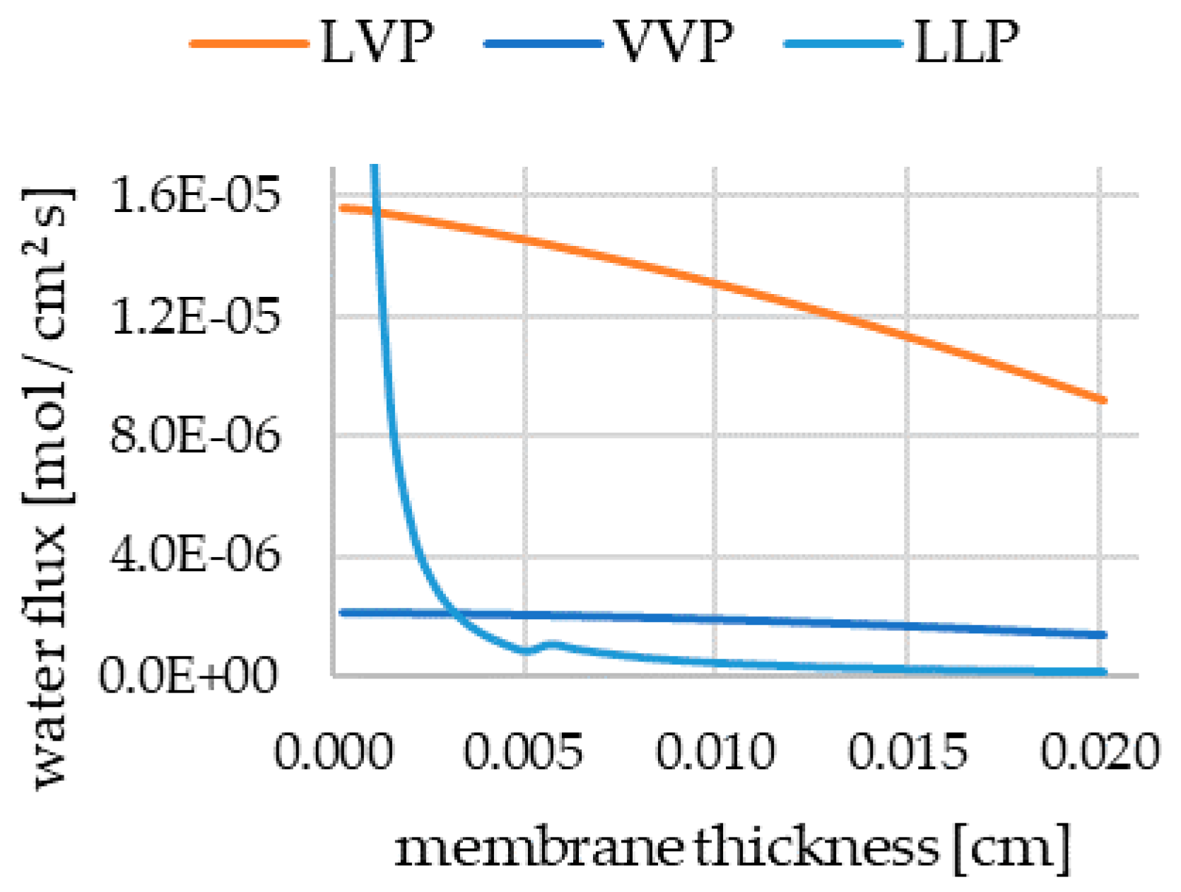
Three major simplifications are applied to reduce the complexity of water transport mechanisms. First, only the flow through the membrane is considered, whilst transport through the porous media of catalyst and gas diffusion layers is neglected. Second, it is assumed that liquid water is only present once the gas mixture is saturated. Finally, liquid and vapor phases are not directly considered. Instead, the chosen equations for diffusive and hydraulic flow are adjusted by several functions (
Figure 2) created with the MATLAB curve fitting application and experimental data from Adachi et al. [
24]. As a result, three cases are described in the following sections: vapor–vapor (VVP), liquid–vapor (LVP) and liquid–liquid permeation (LLP).
2.7.1. Osmosis
Water transport due to osmosis
is expressed by a linear correlation composed of the Faraday constant
, the current
[
11]
and the osmotic coefficient
, which is dependent on the (average) water content of the membrane
[
25]:
2.7.2. Diffusion
In terms of diffusion
, the abovementioned functions to differentiate between the liquid and gaseous phase are utilized. The basis for these calculations is given by [
17]
which considers the cell area
, (average) diffusive coefficient of water
, water concentration gradient
—here: difference between cathode and anode—and membrane thickness
. The latter is treated as a constant (=201 µm) in the above equation and variations are instead considered by the adjustment-functions (Equations (26)–(32)).
To estimate the diffusion coefficient for water through the membrane
, the following expression dependent on membrane temperature
and (average) water content
is applied [
9,
26]:
Subsequently, the diffusive flow
is adjusted for the thickness of the membrane. VVP-correction is applied in the complete absence of liquid water, whilst LVP-correction is used if at least one side is flooded with liquid water. For mixtures of gaseous and liquid phases, a linear scaling is applied:
2.7.3. Hydraulic Permeation
Beyond that, hydraulic permeation is only considered if liquid water is present on both sides of the membrane, since the pressure difference has a minor impact on water vapor transport [
27]. The hydraulic flow
is estimated by a linear correlation with the pressure gradient
—here: difference between cathode and anode—affected by the cell area
, dynamic viscosity of water
as well as water concentration inside the membrane
, its thickness
and hydraulic permeability
[
16]:
For the hydraulic permeability
, a direct dependency on the membrane water content
is assumed [
16]:
Furthermore, the dynamic viscosity of water is approximated by a function of temperature
[
28]
where
denotes a reference value while
,
,
and
are constants. The pressure
has been neglected, since it has a minor impact on
at typical PEMFC operating pressures.
Experimental data suggest a nonlinear relation between the hydraulic flow and membrane thickness [
24], hence an adjustment-function is applied for the hydraulic permeability
at a reference pressure difference of 0.025
:
Subsequently, the hydraulic flow is corrected for the actual pressure difference:
3. Application
Two modes of operation are available for using this model, as displayed in
Figure 3. First, the cell performance can be calculated solely based on physical parameters. Second, the cell performance can be estimated based on the voltage deviation from a supplied polarization table. In the latter case, a distinction can be made between using a single or multiple polarization curves as reference.
For this purpose, the inputs of the MATLAB-function are divided into two categories: one for the state variables mandatory to estimate the cell performance and another for the polarization table references. When running in mode 1, the inputs from the second category are ignored. In mode 2a, the model expects reference values for the experimental conditions of the polarization curve recording. Lastly, in the case of 2b, internal calculations for voltage deviation can be disabled by supplying state variables as table references. e.g., when using polarization curves for different temperatures, supplying the current cell temperature will lead to no additional adjustments for this factor, since current and reference values are identical. The operation mode has no impact on the calculations for concentration overpotential and water transport, however, since these heavily depend on stack composition and media supply.
It is also possible to use this model outside of the MATLAB environment via Co-Simulation. As an example, the program code can be run inside of a MATLAB-Function-block within a Simulink model, which can be compiled as C/C++ code. Depending on the target software, the exact Simulink model composition—regarding inputs, outputs and parameters—and compilation procedure may be wary and has to be looked up in the corresponding documentation. Following this practice allows the fuel cell model to be used in any simulation platform with support for Simulink coupling.
4. Simulation Results
Figure 4 shows a set of polarization curves calculated by the presented model. A variation of the chosen parameters affects the overpotentials and therefore the overall cell voltage (
Section 2). In terms of computational time, creating a polarization curve with hundreds of data points only takes a few s on a modern CPU. This shows the suitability of the model at hand for large system simulations or real-time applications. The inputs and most important parameters for the reference case are represented by
Table 1, and a complete list of all model parameters is supplied as
Supplementary Material.
5. Conclusions
The model at hand represents a one-dimensional, dynamic proton exchange membrane fuel cell. To estimate the cell voltage, activation, ohmic and concentration overpotentials are calculated and subtracted from the ideal cell voltage in every time step. Furthermore, the water transport through the membrane by means of osmosis, diffusion and hydraulic permeation is considered. In order to reduce the complexity and computational load, simplified correlations are used to estimate the cell performance. This approach allows the model to be used in complex systems such as complete vehicle models or real-time applications. Two modes of operation allow for flexible use of the fuel cell model by supplying either polarization tables or physical cell parameters, which enables a quick model setup. The program code is written in MATLAB and designed to be used in a MATLAB-function-block inside of a Simulink model. By compiling the Simulink model as C/C++, this PEMFC model can also be used within any software tool that supports Simulink coupling. It is supplied under an open-access license to make it available to anyone for free.
However, the use of simplified equations for cell performance estimation also reduces the accuracy of the results. In particular, the consideration of the MEA can be further expanded because water and gas transport as well as concentration, can be significantly affected by the MEA composition. Additionally, cell geometry and local differences in the distribution of temperature, current density and reactants can also affect the overall performance. For future expansions, the computational load should be considered, in order to not increase the model’s calculation time too much.
Author Contributions
Formal analysis, investigation, methodology, software, and visualization, writing—original draft, A.L.L.; data curation, S.C.K.; supervision, resources, H.R.; validation, A.L.L. and S.C.K.; writing—review and editing, S.C.K. and H.R.; conceptualization, project administration, A.L.L., S.C.K. and H.R.
Funding
This research received no external funding.
Conflicts of Interest
The authors declare no conflict of interest.
Nomenclature
| water activity |
| catalyst-specific area, cm2/mg |
| constant in the calculation of , bar−1 |
| constant in the calculation of , J/mol bar |
| constant in the calculation of , K/mol bar |
| molar concentration, mol/cm3 |
| membrane water concentration, mol/cm3 |
| diffusion coefficient, cm2/s |
| diffusion coefficient of water through the membrane, cm2/s |
| constant in the calculation of , J/mol |
| voltage, V |
| membrane equivalent weight, g/mol |
| membrane liquid water volume fraction |
| Faraday constant, A s/mol |
| Gibbs free energy, J/mol |
| activation energy, J/mol |
| enthalpy, J |
| current density, A/cm2 |
| exchange current density, A/cm2 |
| reference exchange current density, A/cm2 |
| limiting current density, A/cm2 |
| water flow, mol/s |
| hydraulic permeability of the membrane (liquid water), cm2 |
| hydraulic permeability coefficient (liquid water) |
| catalyst loading, mg/cm2 |
| molar flux, mol/cm2 s |
| number of electrodes involved |
| water transport coefficient |
| power, W |
| pressure, bar |
| partial pressure, bar |
| reference pressure, bar |
| heat flow, W |
| universal gas constant, J/mol K |
| liquid water volume fraction |
| entropy, J/K |
| temperature, K |
| reference temperature, K |
| acid equivalent volume of the membrane, cm3/mol |
| molar volume of water, cm3/mol |
| percentage |
| Greek Letters |
| charge transfer coefficient |
| pressure dependency coefficient |
| thickness, cm |
| electrode porosity |
| efficiency |
| membrane water content |
| reference water dynamic viscosity, Pa s |
| water dynamic viscosity, Pa s |
| density, g/cm3 |
| conductivity, A/V cm |
| electrode tortuosity |
References
- Harvey, D.B.; Pharaoh, J.G.; Karan, K. FAST-FC: Open source fuel cell model: An Open Source Performance and Degradation Fuel Cell Model for PEMFCs. Available online: https://www.fastsimulations.com/source-code.html (accessed on 3 September 2019).
- Falcão, D.S.; Pinho, C.; Pinto, A.M.F.R. Water management in PEMFC: 1-D model simulations. Ciênc. Tecnol. dos Mater. 2016, 28, 81–87. [Google Scholar] [CrossRef]
- Secanell, M.; Putz, A.; Wardlaw, P.; Zingan, V.; Bhaiya, M.; Moore, M.; Zhou, J.; Balen, C.; Domican, K. OpenFCST: An Open-Source Mathematical Modelling Software for Polymer Electrolyte Fuel Cells. ECS Trans. 2014, 64, 655–680. [Google Scholar] [CrossRef]
- Falcão, D.S.; Gomes, P.J.; Oliveira, V.B.; Pinho, C.; Pinto, A.M.F.R. 1D and 3D numerical simulations in PEM fuel cells. Int. J. Hydrog. Energy 2011, 36, 12486–12498. [Google Scholar] [CrossRef]
- Spiegel, C. PEM Fuel Cell Modeling and Simulation Using Matlab; Elsevier: Amsterdam, The Netherlands, 2008; ISBN 978-0-12-374259-9. [Google Scholar]
- Chakraborty, U.K.; Abbott, T.E.; Das, S.K. PEM fuel cell modeling using differential evolution. Energy 2012, 40, 387–399. [Google Scholar] [CrossRef]
- Conti, B.; Bosio, B.; McPhail, S.J.; Santoni, F.; Pumiglia, D.; Arato, E. A 2-D model for Intermediate Temperature Solid Oxide Fuel Cells Preliminarily Validated on Local Values. Catalysts 2019, 9, 36. [Google Scholar] [CrossRef]
- Chakraborty, U.K. A New Model for Constant Fuel Utilization and Constant Fuel Flow in Fuel Cells. Appl. Sci. 2019, 9, 1066. [Google Scholar] [CrossRef]
- Vetter, R.; Schumacher, J.O. Free open reference implementation of a two-phase PEM fuel cell model. Comput. Phys. Commun. 2019, 234, 223–234. [Google Scholar] [CrossRef]
- Chakraborty, U.K. Reversible and Irreversible Potentials and an Inaccuracy in Popular Models in the Fuel Cell Literature. Energies 2018, 11, 1851. [Google Scholar] [CrossRef]
- Barbir, F. PEM Fuel Cells. Theory and Practice, 2nd ed.; Academic Press: Waltham, MA, USA, 2013; ISBN 9780123877109. [Google Scholar]
- Yigit, T.; Selamet, O.F. Mathematical modeling and dynamic Simulink simulation of high-pressure PEM electrolyzer system. Int. J. Hydrog. Energy 2016, 41, 13901–13914. [Google Scholar] [CrossRef]
- Carmo, M.; Fritz, D.L.; Mergel, J.; Stolten, D. A comprehensive review on PEM water electrolysis. Int. J. Hydrog. Energy 2013, 38, 4901–4934. [Google Scholar] [CrossRef]
- Song, C.; Tang, Y.; Zhang, J.L.; Zhang, J.; Wang, H.; Shen, J.; McDermid, S.; Li, J.; Kozak, P. PEM fuel cell reaction kinetics in the temperature range of 23–120°C. Electrochim. Acta 2007, 52, 2552–2561. [Google Scholar] [CrossRef]
- Springer, T.E. Polymer Electrolyte Fuel Cell Model. J. Electrochem. Soc. 1991, 138, 2334. [Google Scholar] [CrossRef]
- Jiao, K.; Li, X. Water transport in polymer electrolyte membrane fuel cells. Prog. Energy Combust. Sci. 2011, 37, 221–291. [Google Scholar] [CrossRef]
- Abdin, Z.; Webb, C.J.; Gray, E.M. PEM fuel cell model and simulation in Matlab–Simulink based on physical parameters. Energy 2016, 116, 1131–1144. [Google Scholar] [CrossRef]
- Chemours. Chemours Product-Bulletin Nafion N115-N117-N1110. Available online: https://nafionstore-us.americommerce.com/Shared/Bulletins/N115-N117-N1110-Product-Bulletin-Chemours.pdf (accessed on 13 May 2019).
- Weber, A.Z.; Newman, J. Transport in Polymer-Electrolyte Membranes. J. Electrochem. Soc. 2003, 150, A1008–A1015. [Google Scholar] [CrossRef]
- Kersting, A.; Aeschbach-Hertig, W. Vorlesungen Physik aquatischer Systeme I. Vorlesung. Available online: http://www.iup.uni-heidelberg.de/institut/studium/lehre/AquaPhys/docMVEnv3_11/MVEnv3_2011_p1_2_Dichte.pdf (accessed on 13 May 2019).
- Musio, F.; Tacchi, F.; Omati, L.; Gallo Stampino, P.; Dotelli, G.; Limonta, S.; Brivio, D.; Grassini, P. PEMFC system simulation in MATLAB-Simulink® environment. Int. J. Hydrog. Energy 2011, 36, 8045–8052. [Google Scholar] [CrossRef]
- Rosén, T.; Eller, J.; Kang, J.; Prasianakis, N.I.; Mantzaras, J.; Büchi, F.N. Saturation Dependent Effective Transport Properties of PEFC Gas Diffusion Layers. J. Electrochem. Soc. 2012, 159, F536–F544. [Google Scholar] [CrossRef]
- Bird, R.B. Transport phenomena. Appl. Mech. Rev. 2002, 55, R1–R4. [Google Scholar] [CrossRef]
- Adachi, M.; Navessin, T.; Xie, Z.; Li, F.H.; Tanaka, S.; Holdcroft, S. Thickness dependence of water permeation through proton exchange membranes. J. Membr. Sci. 2010, 364, 183–193. [Google Scholar] [CrossRef]
- Dutta, S.; Shimpalee, S.; van Zee, J.W. Numerical prediction of mass-exchange between cathode and anode channels in a PEM fuel cell. Int. J. Heat Mass Transf. 2001, 44, 2029–2042. [Google Scholar] [CrossRef]
- Mittelsteadt, C.K.; Staser, J. Simultaneous Water Uptake, Diffusivity and Permeability Measurement of Perfluorinated Sulfonic Acid Polymer Electrolyte Membranes. ECS Trans. 2011, 41, 101–121. [Google Scholar] [CrossRef]
- Karpenko-Jereb, L.; Innerwinkler, P.; Kelterer, A.-M.; Sternig, C.; Fink, C.; Prenninger, P.; Tatschl, R. A novel membrane transport model for polymer electrolyte fuel cell simulations. Int. J. Hydrog. Energy 2014, 39, 7077–7088. [Google Scholar] [CrossRef]
- Likhachev, E.R. Dependence of water viscosity on temperature and pressure. Tech. Phys. 2003, 48, 514–515. [Google Scholar] [CrossRef]
© 2019 by the authors. Licensee MDPI, Basel, Switzerland. This article is an open access article distributed under the terms and conditions of the Creative Commons Attribution (CC BY) license (http://creativecommons.org/licenses/by/4.0/).


