Identification of Noise, Vibration and Harshness Behavior of Wind Turbine Drivetrain under Different Operating Conditions

Abstract

Noise, vibration and harshness (NVH) problems are critical issues to be tackled for wind turbine drivetrains. Tracking the behavior of modal parameters of the machines’ fundamental modes during operation it is of high interest to validate complex simulation models. A powerful approach for this purpose is represented by operational modal analysis (OMA). This paper describes the investigation of an automated technique for continuously tracking the modes of a rotating mechanical system running in normal operating conditions. The modal estimation procedure is based on an automatic version of the pLSCF (poly-reference Least-Square Complex Frequency-Domain) algorithm. The latter is coupled with a method that automatically tracks the modal parameters along different data sets. The use of OMA on a rotating component of the wind turbine creates the need to deal with harmonics in order to satisfy one of the assumptions of OMA. For this purpose, the use of a cepstrum editing procedure is analyzed and implemented. Modal estimates obtained from an automated analysis on stand still data and normal operating conditions data are compared, to test the added value of the cepstrum editing procedure and the robustness of the method when used on real data. To illustrate and validate the implemented methodology, data acquired during a long-term monitoring campaign of a wind turbine drivetrain are used.

1. Introduction

1.1. Motivation

The susceptibility of structures to vibrations and the generation of tonalities is one of the main design issues in the field of rotating machinery. For this reason, eigenfrequencies, damping ratios, mode shapes and modal scaling factors are fundamental parameters for the design. The experimental validation of the values obtained with simulations is essential for model validation and for guaranteeing the safety and reliability of the structure [1]. Since damping and boundary conditions depend on the vibration amplitude and modal parameters depend on the (rotating) speed of the machine and its parts, it is important to experimentally verify the design values in normal operating conditions, that is, around operating points. Industrial design processes currently comprise full-scale machine testing and component-level-testing both in field and laboratory environments. While these tests ensure good observability and precise estimated models due to the limited number of components/machines tested allowing the use of a significant number of sensors, they are generally performed over short time spans trying to catch specific operating conditions of interest.

To solve all noise, vibrations and harshness (NVH) problems and avoid inefficiently optimized machines and higher operational and maintenance costs, it is necessary to have insights into the behavior of machines during their overall lifetime and for each important operating condition [2]. Moreover, since tonalities depend on the transfer path of vibrations through the overall structure [3], the optimization of NVH behavior leads to a reduction of the noise generated by the turbines, ensuring the respect of the legislation [4]. An evolution of the current industrial process is represented by a new kind of design technique that learns from the information acquired on several machines that are already in service and takes decisions on how to improve models. This paper wants to introduce a methodology—named field data-driven design—that, based on advanced vibration analysis combining signal processing and machine learning algorithms, provides the information needed to easily understand the undesirable behavior of the structure and its consequences.

This research focuses then on the identification of the modal parameters of an operating wind turbine drivetrain. Allowing the extraction of the modal parameters from the dynamic response of the structure to unmeasured operational forces, operational modal analysis (OMA) serves as an effective approach at this purpose. However, OMA is built on several assumptions which are not always fulfilled in case of rotating machines. This is the main reason why in the last years researchers started exploring new techniques. An interesting overview of the limits of OMA when applied to complex machines such as wind turbines is given in Reference [5].The main issues affecting the use of OMA for rotating machines are linked to the characteristics of the system under analysis that violates two main assumptions OMA is based on. Since wind turbines consist of subcomponents moving one with respect to the other (e.g., pitch systems), the structure can not be considered time invariant; secondly the presence of rotational components in the excitation forces, makes the assumption of white noise spectrum input violated as well. As stated, several authors are working to push the limits of OMA techniques. In Reference [6], the authors show a technique to address the described problem in the analysis of a wind turbine foundation. The described method has the same objective as this paper: long term dynamic characterization of a structure by means of automated long term operational modal analysis. However, authors that try to adopt this technique on drivetrains still have to overcome a research gap. As described in Reference [7], operational modal analysis on wind turbine drivetrains needs additional attention for several reasons. First of all the number of components in the nacelle that produce vibration harmonics are not negligible—generator, pitch-drive and the yaw-drive. The amount of harmonic components in the signal makes not trivial the separation of the harmonics from the structural modes. Moreover, considering the high frequency band of interest (well above 100 Hz) the structural modes of the gearbox are generally in a frequency band excited by the faster gear stages in which the harmonics are predominant and highly affected by speed variation. Secondly, the complexity of the system under analysis—the gearbox itself has many parts, each featured by modal parameters. Therefore the modal density is significantly high, making the automation of the modal parameter estimation more challenging; moreover, once the parameters have been estimated for one dataset, it becomes difficult to distinguish whether close estimates represent the same mode with shifted modal parameters or two separated (crossing) modes.

This paper wants to propose a method to overcome the mentioned research gap that still needs to be addressed in order to adopt long term operational modal analysis for the identification of modal parameters of a wind turbine drivetrain.

1.2. Field Data-Driven Design

In Reference [5] the authors suggest some methods to deal with the limits of OMA. Concerning the time-variance of the system, they face the variation of yaw and pitch angles by analyzing periods of time when these angles change insignificantly or by performing a simple coordinate transformation in order to account for yaw angle and by averaging characteristic value of pitch angle; for dealing with rotor rotation they suggest to include the rotation into the equations of motion of entire wind turbine. In this paper, a different approach is presented. The main reason that led the authors to look for a different solution, is the will of solving this problem by facing it with a data-scientific approach and significantly reduce the influence of making assumptions and calculations on the final results. The objective is to deal with the time invariance of the system by looking at sub-datasets that are short enough for the system to be considered time-invariant and track the modal parameters extracted from the sub-dataset with respect to the data available from SCADA (i.e., supervisory control and data acquisition) system, representative for the operating conditions. In this way it is possible for the analyst to directly link anomalous behavior to specific operating conditions or to structural problems. This topic is particularly interesting for wind energy applications. Due to the extreme environment in which wind turbines operate, machines and components are subjected to highly variable operating conditions that cause important mechanical stresses [8]. For this reason, the drivetrain has been already analized for long periods as described in References [9,10]. The referenced works, however, analyze the drivetrain in stand still condition. This approach is close to what is suggested in Reference [5]—a particular operating condition has been selected in order to be able to consider the system as time invariant. Moreover the choice of stand still data does not introduce the problem of harmonics—in this condition, harmonics do not dominate the frequency band of interest and OMA can be performed in a reliable way, without any pre-processing needed. The work presented in this paper wants to be an extension of what has been already done—considering normal operating conditions, the variability of the system and the presence of harmonics are introduced. The objective is then to propose methodology for facing these challenges and observe the dynamic behavior of the drive train continuously and independently from the operating conditions.

For dealing with harmonics components in the input signal the methodology has been chosen and implemented in order to minimize the influence of the analyst and make autonomous the analysis of the data. Cepstrum based harmonics lifter is a pre-processing methodology extensively described in the literature [11,12,13,14,15,16] that resulted to be the highly suitable to be automatized.

In order to achieve the goal of this research, an algorithm that allows a continuous tracking of the modal parameters in time is built. The algorithm is shown by means of the block diagram in Figure 1. The algorithm starts with a classification of the data based on their operating conditions. Since the main discriminant in this methodology is the rotational speed, datasets of raw data are classified as stand still data (turbine in parked conditions) and rotating data (turbine producing energy). A third category of data is identified—the data where the turbine is running up or coasting down. This data are not considered by the algorithm as it is, but it is intention of the authors to further investigate a procedure that allows an analysis of this kind of data (named Order Based Modal Analysis). Once the data are classified they go through different procedures depending on their nature—rotating data are pre-processed by means of a cepstrum based harmonics filter. A brief description of the operating principle of this method is given in Section 2, while the main contributions of this work with respect to this part are explained in Section 3.1 and Section 3.2 where the investigation of the effect of different filters and the description of the algorithm that automatically selects the cutoff-quefrency, main parameter of the cepstrum lifter, are given.

After the data are prepared for modal analysis, they are processed by means of an automatic OMA algorithm. A description of classic OMA is given in Section 2 and the automation of the algorithm is described in Section 3.3. This algorithm allows the extraction of the modal parameters for each dataset. The final step of the analysis is thus the tracking of the modal parameters extracted from different dataset, representing the evolution of the natural frequencies and damping ratio in time and for different operating condition. This method is described in Section 3.4.

2. Theoretical Background

As already stated, the direct use of OMA on vibration data coming from rotating systems gives erroneous results. Therefore, classical OMA methods are extended to be used in presence of harmonics in the input signals. These methods either assume the knowledge of the disturbances’ frequency or identify the harmonics via noise poles on the unitary circles [17]. These methods assume the stationarity (constant amplitude, frequency and phase) of the harmonic frequencies. However, most of the practical applications such as diesel motors, turbines and helicopters violate this assumption—the speed variations are not negligible and therefore harmonics influence broader frequency bands, since they are smeared in the spectrum of the signals. As a consequence the harmonic components can not be modeled accurately with the mentioned methods and the modal parameters extraction fails whenever the time varying frequency is close to a resonance [17].

A possible solution is to add in the analysis a pre-processing step to remove harmonic components from the raw before using classical OMA algorithms. Basic signal processing techniques for filtering harmonics are listed in References [12,16]. Another possibility is to perform the parameter estimation on tracked orders rather than on the overall spectrum, implementing the so called order based modal analysis (OBMA) [18]. As the basis of this technique there is the idea that during run-up or coast-down of the machine, the measured responses are mainly caused by rotational excitations, which are considered to be multi-sine sweep excitations in the frequency band of interest. However the goal of this work is the analysis of the system in normal operating conditions, therefore the most appropriated procedure is filtering the harmonics out of the raw data. For this purpose cepstrum editing procedure is adopted to reduce the influence of the harmonics from the signal.

Cepstrum analysis was defined in 1963 [19] as the "Power spectrum of the logarithm of the power spectrum". It has been formulated as a method for detecting echoes in seismic or speech analyses. The original formulation of the (power) cepstrum is:

$$C_p\left(\tau \right)={\left|\mathcal{F}\left\{log\left(F_{xx}\left(f\right)\right)\right\}\right|}^2$$

(1)

where $\mathcal{F}$ is the Fourier transform operator, $F_{xx}\left(f\right)$ is the power spectrum of the signal, $\tau$ is the cepstrum domain vector and f the frequency vector.

The definition of the complex cepstrum is:

$$C_c\left(\tau \right)={\mathcal{F}}^{-1}\left\{log\left(F\left(f\right)\right)\right\}={\mathcal{F}}^{-1}\{ln\left(A\left(f\right)\right)+j\mathsf{\Phi }\left(f\right)\}$$

(2)

where:

$$F\left(f\right)=\mathcal{F}\left\{f\left(t\right)\right\}=A\left(f\right)e^{j\varphi \left(f\right)}$$

(3)

in terms of amplitude ($A\left(f\right)$) and phase ($\varphi \left(f\right)$) of the spectrum.

The new power cepstrum, is given by:

$$C_p\left(\tau \right)={\mathcal{F}}^{-1}\left\{log\left(F_{xx}\left(f\right)\right)\right\}$$

(4)

which for the spectrum of a single record (as in Equation (3)) can be expressed as:

$$C_p\left(\tau \right)={\mathcal{F}}^{-1}\left\{2ln\left(A\left(f\right)\right)\right\}$$

(5)

The so-called real cepstrum is obtained by setting the phase to zero in Equation (2):

$$C_t\left(\tau \right)={\mathcal{F}}^{-1}\left\{ln\left(A\left(f\right)\right)\right\}$$

(6)

which is simply a scaled version of Equation (5).

Cepstrum became a powerful approach for editing time-domain signals when the possibility of going back to the time domain was introduced and after that is has been realized that modifying the amplitude only (i.e., using the real cepstrum) was sufficient [20]. The edited time-domain signal can be generated combining the modified amplitude spectrum with the original phase spectrum to generate the edited time-domain signal.

Bringing time-domain signals in the quefrency domain concentrates the families of harmonics in single lines rahmonics. To remove family of harmonics in the time-domain it is enough to set rahmonics lines to zero. The use of this method as a pre-processing for OMA finds its reason in the fact that the information about the modes is concentrated at low quefrencies [11]. Therefore the use of a short-pass lifter in the quefrency domain allows to keep the modal information of the signal largely intact while removing all the components at higher quefrencies.

Resampling the signal to angular domain before expressing it to the cepstrum domain, allows to have narrower rahmonics. since it has not been shown that resampling the signal does not bring advantages in the use of a cepstrum lifter, two different possibilities are investigated—the application of the cepstrum lifter to both time and angular domain signals. It has been shown that resonances, not tied to the speed of the shaft, are altered by the angular resampling operation [21]. Therefore, after the use of the cepstrum lifter on the raw angular-domain signal, the latter is brought back to the time domain (i.e., samples every $\mathsf{\Delta }t$ seconds, with $\mathsf{\Delta }t$ being the time samples spacing).

Once raw data are made suitable for the use of classic OMA algorithms, modal parameters are estimated. The Poly-reference Least-square Complex Frequency-Domain method (p-LSCF) is used. This algorithm is based on the use of the right matrix model to extract the modal parameters from measured data. The original algorithm makes use of the stabilization diagram from which the analyst has to identify and select the physical poles on the stabilization diagram, a diagram that shows the poles identified by fitting the measured data with increasing order models. Amongst all the possible OMA algorithms [22], this method has been chosen because it estimates the poles with negative damping ratio as non-physical poles excluding them from the stabilization diagram [23], that results to be clearer. However, the method still requires an extensive algorithm-analyst interaction represented by the selection of the physical poles on the stabilization diagram. This is inappropriate if continuous modal parameters tracking wants to be performed automatically on a a stream of data. For this reason an automatic version of this algorithm is introduced and described in Section 3.3.

3. Methodology

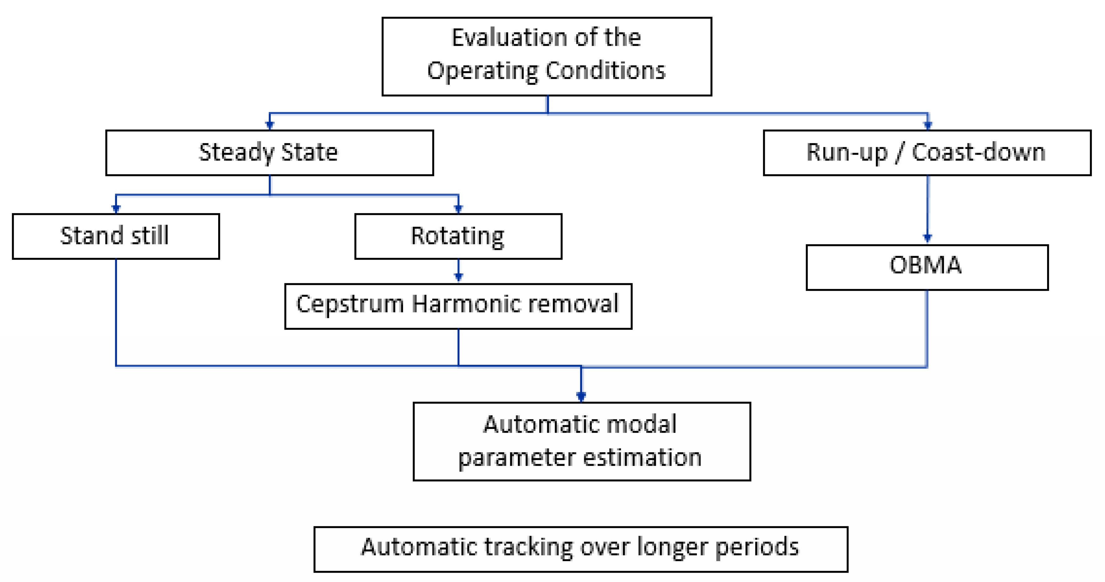
Cepstrum editing procedure must be combined with automated modal parameters estimation and tracking algorithms in order to perform automatic OMA on continuous stream of data coming from a wind turbine drivetrain in real operating conditions. This section describes the methodologies listed in Figure 1 with specific attention to automation of the different procedures.

3.1. Selection of the Cepstrum Lifter

To remove the harmonics, the state-of-the-art algorithm described in Section 2 is implemented. The use of two different low pass lifters in the quefrency domain is investigated—exponential and rectangular. While the rectangular lifter truncates the cepstrum domain signal without influencing its decay, the exponential one adds a known amount of damping in the edited signal. This additional damping can be removed from the estimates by means of the following equation [24]:

$${\xi }_r={\xi }_m-\frac{1}{2\pi f_r\tau }$$

(7)

where, for each estimated mode, ${\xi }_r$ is the real damping $[-]$, ${\xi }_m$ is the measured damping $[-]$, $f_r$ is the real frequency $\left[Hz\right]$ and $\tau$ is the time constant of the exponential window $\left[s\right]$. However it has to be noticed that Equation (7) cannot be used if an angular resampled signal is edited with the cepstrum lifter, due to the fact that the angular cepstrum domain is not equivalent anymore to the time-domain cepstrum.

A pre-analysis using a synthesised signal is performed in order to investigate the optimal low pass filter to be applied to the cepstrum domain signal. The generated signal aims to simulate a real structure, featured by transfer path $H\left(s\right)$.

$$H\left(s\right)=\frac{1}{s^2+2\xi {\omega }_{n}s+{\omega }_n^2}$$

(8)

A three modes system is simulated, with the modal parameters listed in

Table 1. Modal parameters of the simulated system.

	Natural Frequency (Hz)	Damping Ratio (%)
Mode 1	50	1
Mode 2	101	1
Mode 3	154	1

:

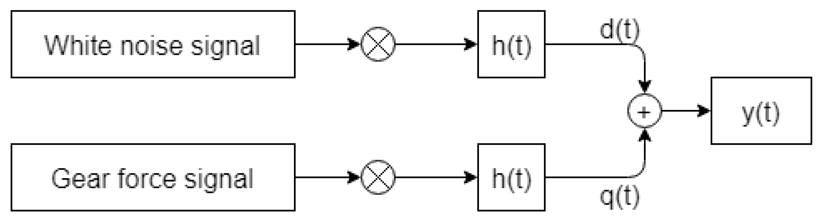
The system is excited by two sources:

• Gear force signal with 20 harmonics of the fundamental 10 Hz;
  $$x_{harm}\left(t\right)=\sum _{n=1}^N(A_n\left(t\right)\sin \left(n\varphi \left(t\right)\right)with\varphi \left(t\right)={\int }_t\omega \left(t\right)dt$$

  (9)

  where N is the number of harmonics, n the harmonic number, $A_n\left(t\right)$ the instantaneous amplitude, $\varphi \left(t\right)$ the instantaneous phase and $\omega \left(t\right)$ the rotational speed.
• White noise signal.
  $$x_{wn}\left(t\right)=e\left(t\right)\in \mathbb{N}(0,{\sigma }^2)$$

  (10)

  where $e\left(t\right)$ is white Gaussian noise normally and independently distributed signal.

The final signal is then given by the sum of two time domain signals:

$$y\left(t\right)=q\left(t\right)+d\left(t\right)$$

(11)

where, being $h\left(t\right)$ the time domain impulse response of the system,

$$\left\{\begin{array}{c}q\left(t\right)=x_{harm}\left(t\right)\otimes h\left(t\right)\hfill \\ d\left(t\right)=x_{wn}\left(t\right)\otimes h\left(t\right)\hfill \end{array}\right.$$

(12)

A schematic explanation of the simulated signal is shown in Figure 2. In Equation (12) and Figure 2 the symbol ⊗ represents the convolution between two signals.

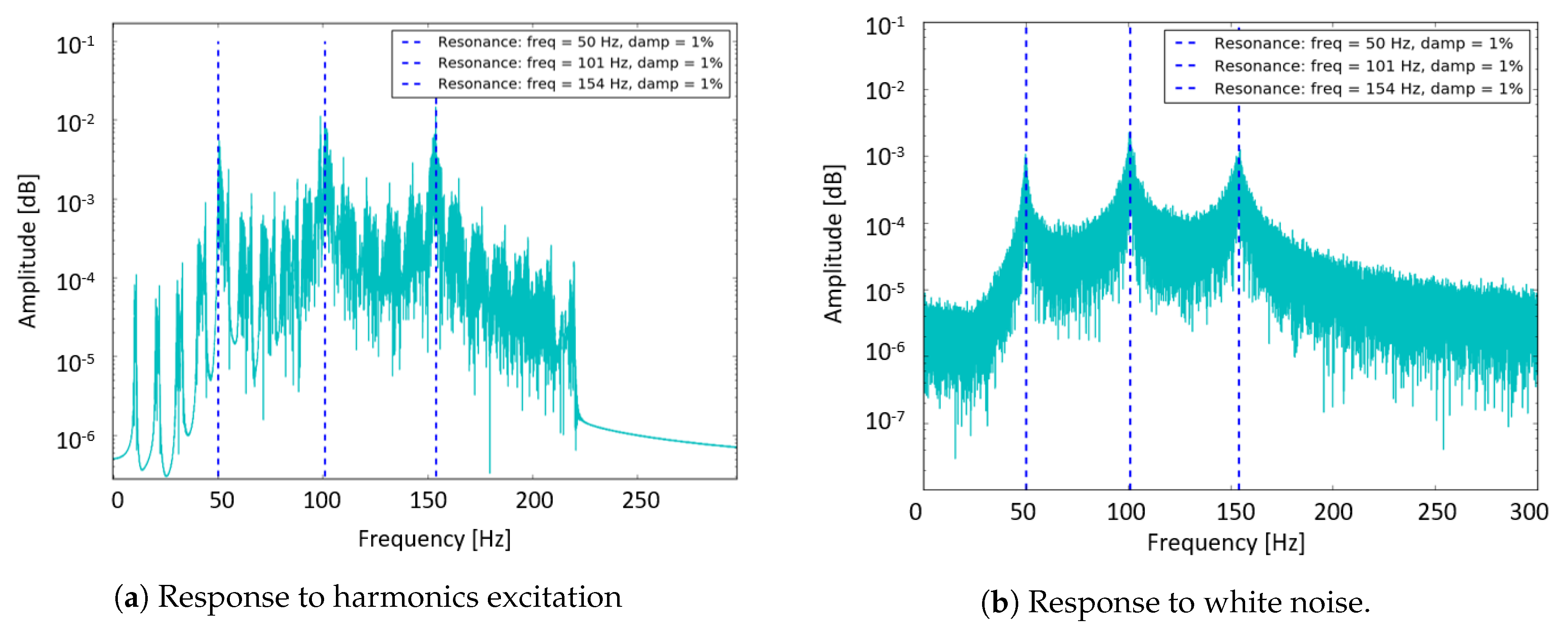
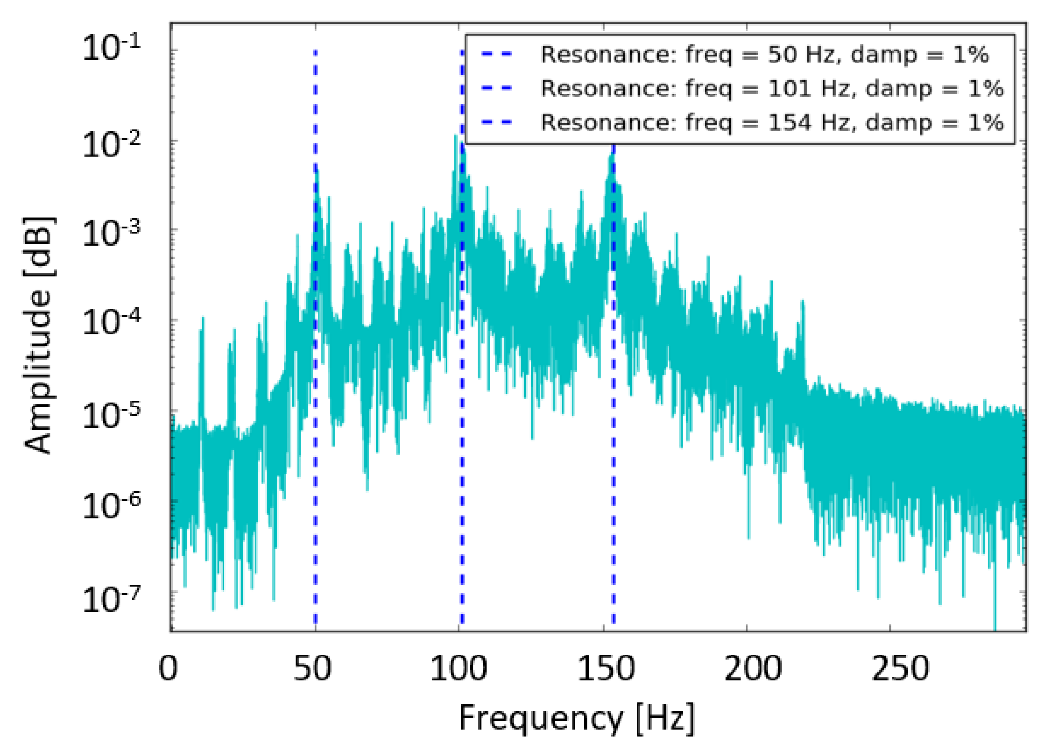
In Figure 3 the two different components of the signal are shown: response to harmonic excitation (Figure 3a, $q\left(t\right)$ in Equation (12)) and response to white noise (Figure 3b, $d\left(t\right)$ in Equation (12)). In Figure 4, the global signal is shown.

The purpose of analyzing this synthesized signal is to test different lifters that can be used—exponential and rectangular lifters applied to time and angular domain signals. After the cepstrum editing procedure, classic OMA is used to verify the validity of the different adopted procedures by means of a comparison of the estimated modal parameters with the expected ones.

To prepare the data for OMA, the periodogram approach [25] is used on the edited signals. The analysis is performed for signals with speed varying around a mean value by amounts of 2% (

Table 2. Results from the use of different cepstrum lifters on the simulated signal when the speed has a 2% variation. Red results are the ones showing values closest to the expected ones.

Time Exponential			Angle Exponential		Time Rectangular		Angle Rectangular
Freq (Hz)	Damp (%)		Freq (Hz)	Damp (%)	Freq (Hz)	Damp (%)	Freq (Hz)	Damp (%)
	Estimated	Corrected
Cutoff Quefrency = 0.05
50.21	6.49	0.16	49.78	5.2	48.73	2.31	49.97	0.91
100.82	3.93	0.77	101.32	0.99	102.56	1.31	101.43	1.12
154.26	2.95	0.9	153.92	2.41	156.01	0.97	154.00	1.13
Cutoff Quefrency = 0.1
50.06	2.63	−0.54	49.94	2.74	49.86	1.05	50.02	0.95
100.38	1.93	0.34	100.88	1.88	100.72	0.94	100.92	0.98
154.693	1.86	0.83	153.98	1.73	153.56	1.07	153.99	1.05
Cutoff Quefrency = 0.2
49.96	0.89	−0.7	49.99	1.66	50.00	0.08	49.99	0.90
100.31	0.93	−0.13	100.99	1.24	100.52	0.27	100.99	0.95
154.20	1.09	0.58	153.88	1.34	153.50	0.18	153.86	0.99

), 10% (

Table 3. Results from the use of different cepstrum lifters on the simulated signal when the speed has a 10% variation. Red results are the ones showing values closest to the expected ones.

Time Exponential			Angle Exponential		Time Rectangular		Angle Rectangular
Freq (Hz)	Damp (%)		Freq (Hz)	Damp (%)	Freq (Hz)	Damp (%)	Freq (Hz)	Damp (%)
	Estimated	Corrected
Cutoff Quefrency = 0.05
50.20	6.70	0.35	49.83	4.28	47.67	3.07	49.93	1.41
101.38	3.96	0.82	101.16	2.54	101.69	1.61	100.92	1.16
154.30	2.96	0.89	153.89	2.10	155.06	1.60	153.91	1.15
Cutoff Quefrency = 0.1
50.54	3.09	−0.05	49.92	2.36	50.95	0.88	49.91	0.97
101.17	2.38	0.80	101.10	1.60	101.20	1.08	101.02	1.05
153.99	1.74	0.72	153.99	1.56	153.92	0.72	153.99	1.10
Cutoff Quefrency = 0.2
50.20	4.70	3.52	49.82	4.28	50.72	0.45	49.87	0.9
101.38	3.96	2.39	101.17	2.54	101.44	0.78	101.08	0.99
154.30	2.96	1.94	153.86	2.10	153.90	0.44	154.07	0.99

) and 15% (

Table 4. Results from the use of different cepstrum lifters on the simulated signal when the speed has a 15% variation. Red results are the ones showing values closest to the expected ones.

Time Exponential			Angle Exponential		Time Rectangular		Angle Rectangular
Freq (Hz)	Damp (%)		Freq (Hz)	Damp (%)	Freq (Hz)	Damp (%)	Freq (Hz)	Damp (%)
	Estimated	Corrected
Cutoff Quefrency = 0.05
50.51	6.9	0.60	49.65	4.54	48.64	3.48	50.10	0.99
100.67	4.30	1.13	100.96	2.40	100.51	1.12	100.89	1.07
154.32	2.68	0.65	154.08	1.84	155.87	1.32	154.30	1.04
Cutoff Quefrency = 0.1
49.82	3.12	−0.07	49.72	2.01	50.35	0.09	50.07	0.94
100.54	2.90	1.32	101.05	1.62	100.58	0.36	101.11	0.99
14.16	1.70	0.60	154.08	1.43	154.17	0.64	154.77	1.05
Cutoff Quefrency = 0.2
49.54	1.73	0.13	49.91	1.15	49.41	0.66	49.96	0.91
100.55	2.00	1.20	100.91	1.30	100.48	1.50	100.90	0.94
154.13	1.15	0.63	154.03	1.25	154.03	0.64	154.00	0.98

). When an exponential window is used in the cepstrum of the time domain signal (first column in the tables), the damping estimates are corrected with Equation (7) to take into account the additional damping introduced by the use of the lifter. Both the values are shown, the estimated one (on the left side) and the corrected one (on the right side). The analyses are performed for different values of the cutoff quefrency, that is, the time constant of the low pass lifter applied in the cepstrum domain. This will help in investigating the influence of this parameter, for which a more thorough analysis is shown in Section 3.2.

Some comments are required on the results shown in Table 2, Table 3 and Table 4. First of all, the estimated frequency and damping values closest to the expected ones are highlighted (i.e., values in red); this helps in understanding what procedure performs best. Results show the non correct estimation of the damping in case an exponential lifter is used on an angular domain signal. This is expected since, as already stated, the damping introduced by the exponential window can not be corrected with Equation (7). However in case the exponential lifter is applied on a time domain signal, the results are also less accurate; after the use of Equation (7) negative damping values are obtained. This is physically impossible because it would lead to an unstable system. Looking at the results obtained with the rectangular window, it can be concluded that resampling raw data helps in improving the estimates of the damping.

Based on these observations, the use of rectangular lifter on an angular resampled signal is selected for processing real data.

3.2. Automatic Selection of the Cutoff Quefrency

Since the objective of this research is to make the algorithm autonomous, this section focuses on the description of a method that allows an automatic selection of the parameter needed by the cepstrum editing procedure—the cutoff quefrency.

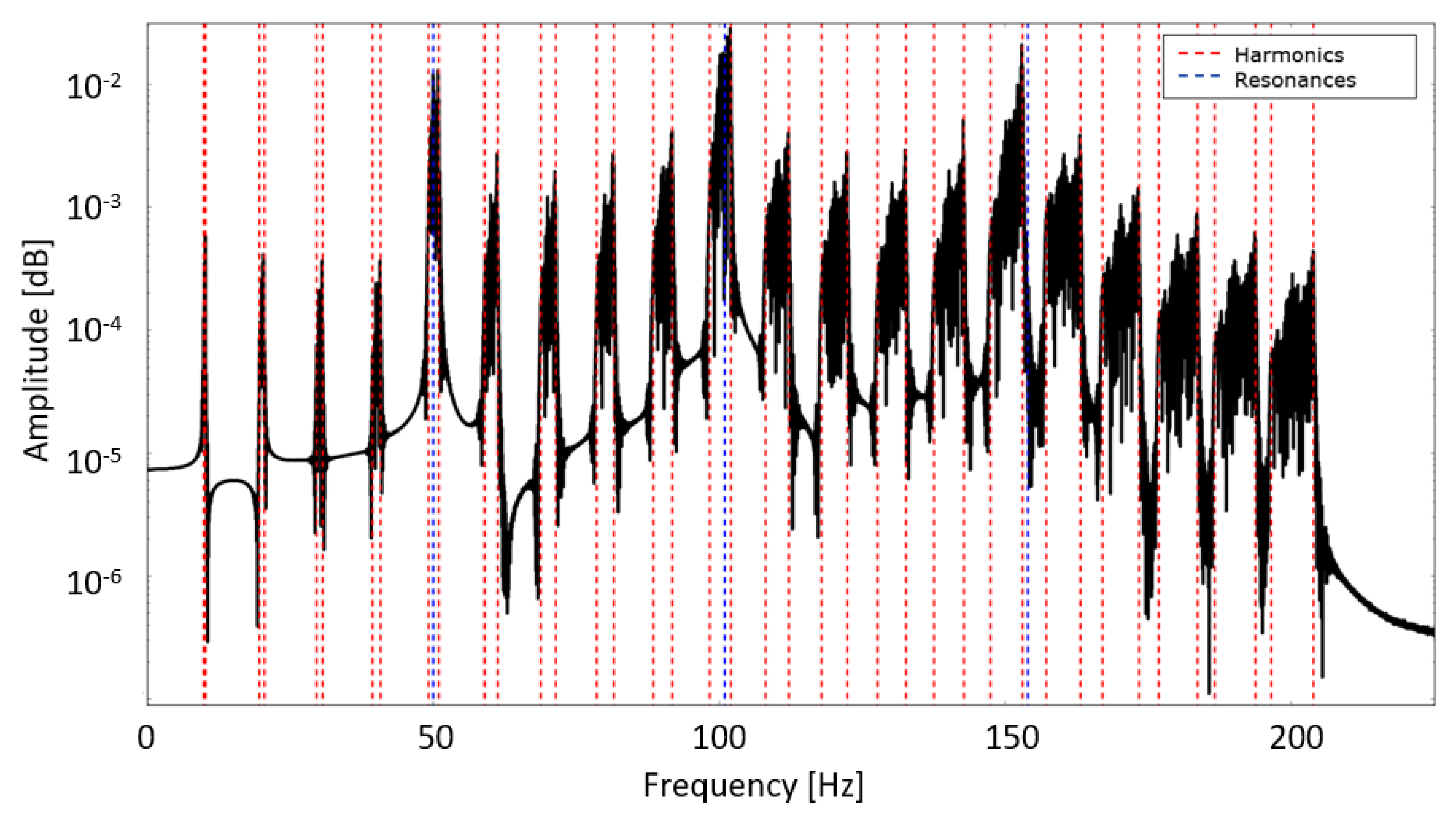
Figure 5 represents the original signal processed with the periodogram algorithm, with the objective of showing the presence of harmonics, and their influence in the spectrum (red lines). The latter is calculated using Equation (13), where $f\left(t\right)$ is the variation of the frequency in time, O is the order of the machine and $\omega \left(t\right)$ the rotational speed. Blue lines in Figure 5 represent the three resonance frequencies.

$$\mathit{f}\left(t\right)=\mathsf{O}\times \frac{\omega \left(t\right)}{2\pi }$$

(13)

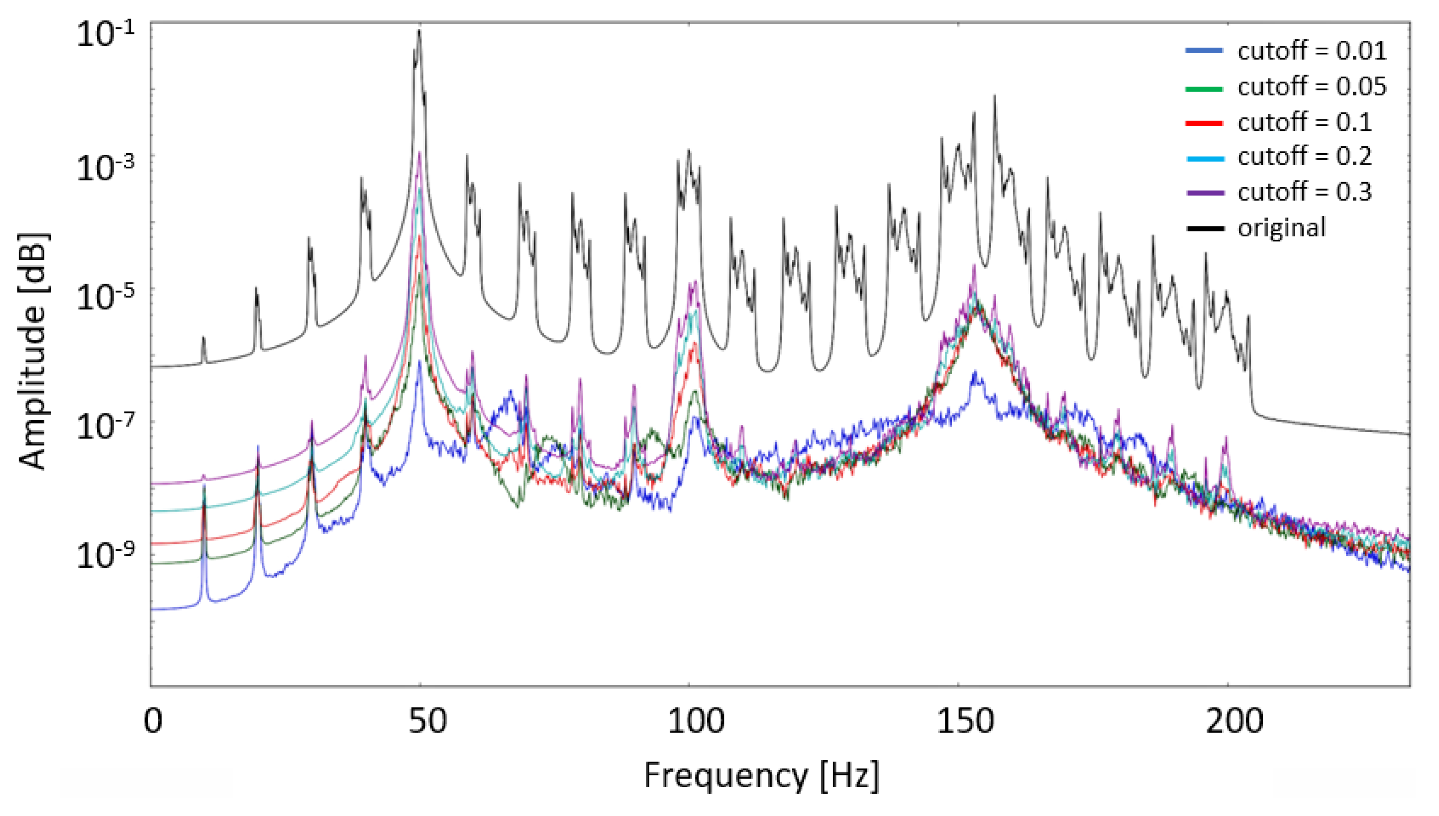
In Figure 6, the iterative use of the cepstrum editing procedure is shown. Decreasing cutoff quefrency values are used. From Figure 6 it can be noticed how higher values of the cutoff quefrency preserve the resonance content, but do not reduce the harmonic-related peaks, while lower values of the cutoff quefrency overly distort the resonances.

The algorithm for the choice of the optimal time constant, is based on the combination of two approaches.

The first one is more empirical and is based on the reduction of the total power introduced by the harmonics. Considering Parseval’s theorem, the latter is calculated with Equation (14) applied in each frequency band that is influenced by harmonic content:

$$P_f=\frac{1}{N}\sum _{k=0}^{N-1}{\left|X\left[k\right]\right|}^2$$

(14)

where $X\left[k\right]$ is the discrete Fourier transform, k is the frequency bin number and N the number of samples. The iterative procedure stops when the amount of energy introduced by the harmonics is 10% of the original value, that is, the energy calculated before applying the cepstrum editing procedure. The choice of this limit value must be defined considering the system under analysis and using a rough prediction on how much the harmonics influence the signal. This procedure presents a disadvantage—if the cutoff quefrency needed to ensure the required energy reduction is too low, it is possible to introduce a distortion in the modal content of the signal. In order to avoid this, the method is coupled with a second algorithm that allows to set a lower bound for the cutoff quefrency value.

This second approach is more theoretical. In Reference [26] it is shown that the damped exponentials are additionally weighted by $1/n$ in the cepstrum domain. Knowing this, it is possible to estimate at which quefrency value the modal content has mostly died out. Of course, to calculate it, information on the frequency and damping of the expected modes must be a priori known, that is not the case in most real applications. Moreover, this is valid only when considering a single degree of freedom system—in the cepstrum domain the contributions of each mode cannot be simply summed (as in the time domain) due to the use of the logarithmic function. However, considering Equation (15) [26] it can be shown that the mode that declines slower in the quefrency domain is the one with a lower frequency. So if the knowledge of the system under analysis allows to roughly estimate a priori the lower expected resonance frequency and the average damping of the structure, it is possible to have an idea of the minimum value of the cutoff quefrency that does not introduce much distortion in the modal content of the signal.

$$\begin{array}{cc}\hfill c_{sdof}\left(n\right)=\frac{c^n}{n}+\frac{c^{*n}}{n}& =\frac{{\left|c\right|}^n}{n}\left[exp\left(jnarg\right(c\left)\right)+exp(-jnarg(c\left)\right)\right]\hfill \\ & =2\frac{e^{-\sigma n\Delta t}}{n}\cos \left(narg\left(c\right)\right)\hfill \end{array}$$

(15)

where n is the quefrency sample number, $\mathsf{\Delta }t$ is the time sample spacing (so that $t=n\mathsf{\Delta }t$), and $\sigma$ is the damping constant corresponding to the exponential decay ${\left|c\right|}^n$.

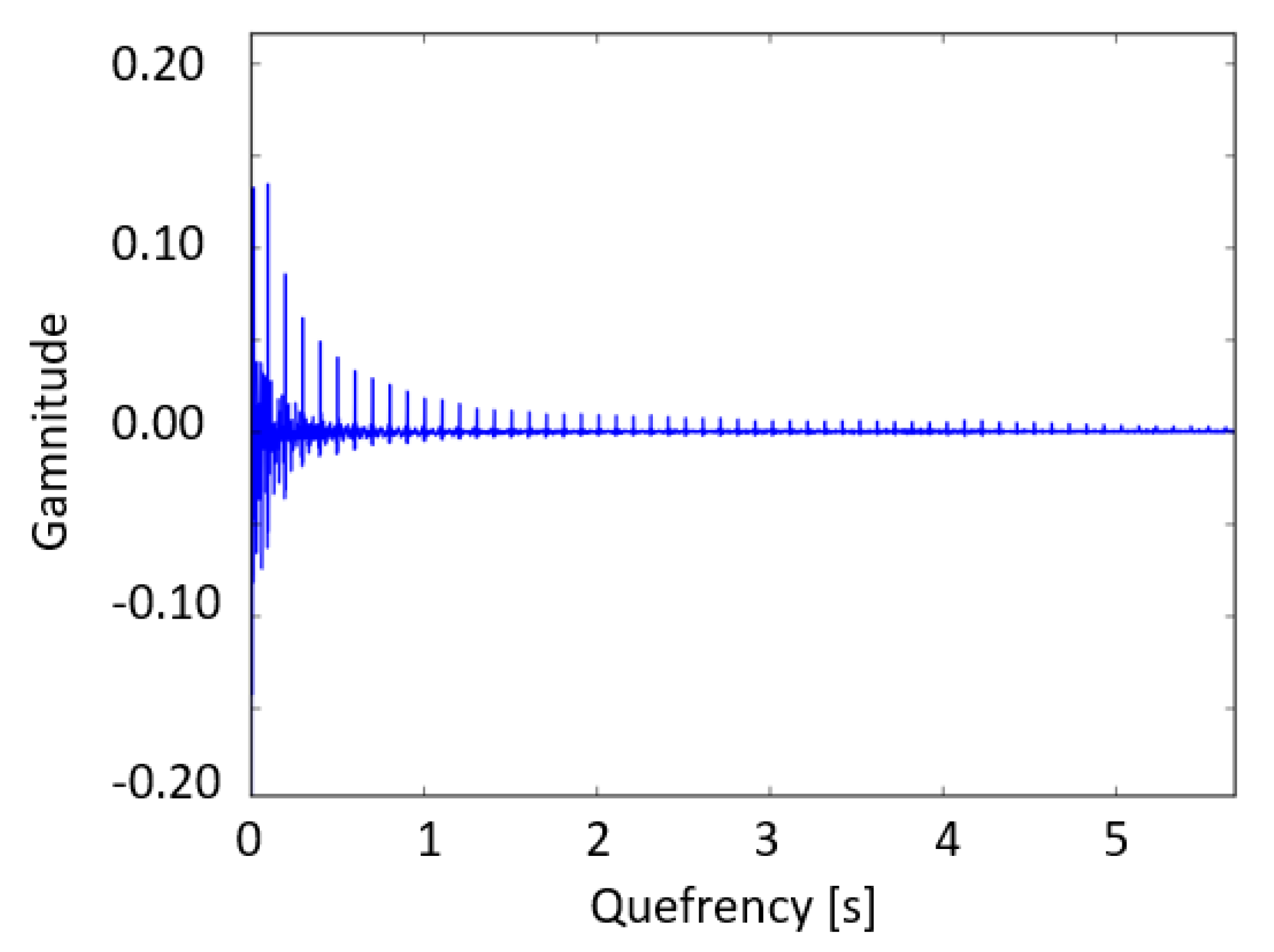
Figure 7 shows the cepstrum of the simulated signal, illustrating the clear distinction of the two regions in the quefrency domain—one containing the modal content and one containing the peaks related to rahmonics. In Figure 7 it is possible to notice how the rahmonics are also present in the modal content region. This makes clear why the definition of this parameter is so critical.

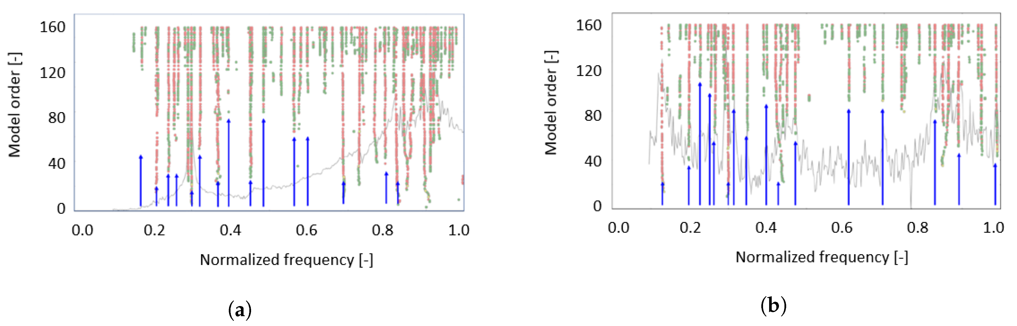
3.3. Automatic Modal Parameter Estimation

As explained in Section 2, the extraction of the modal parameters by means of OMA requires the selection of physical poles from the stabilization diagram. Originally this action was demanded of the analyst, that through an interactive stabilization diagram was able to discriminate the spurious poles from the physical ones, in order to allow the algorithm to synthesize a correct transfer function. However, an automatic selection of the physical poles from the ones represented on the stabilization diagram started to be investigated for several reasons; first of all, to reduce the dependency of the accuracy of the estimation on the level of expertise and reduce this source of uncertainty [27,28]; secondly to allow the analysis of big amount of data continuously. The implementation of fuzzy logics, heuristic rules and clustering analysis as methods to group the modes with similar characteristics [29,30,31,32] can be used as valid solution to make a distinction between spurious and physical poles. Since the method described in Reference [33] resulted in being robust and systematic, it has been adopted in this work. This method uses clustering algorithms in three steps:

• Separation of certainly spurious and possibly physical poles based on single mode validation criteria;
• Grouping the possibly physical poles in separated clusters;
• Selection of the clusters containing physical modes

The authors focused their attention on finding methods to extract the parameters required by the analysis of the data itself.

3.4. Automatic Modal Parameters Tracking

The tracking procedure has been implemented as a comparison between the modal parameters estimated for each data set with a reference set of modes, as investigated in Reference [9]. For the procedure, a reference data set is identified and the relative modal parameters are estimated. The latter are used as reference set to be compared with the modal parameters estimated from the other data sets. The comparison is made measuring in which extent the estimated set of modes is coherent to the reference one terms of frequency/damping values (using poles values) and mode shapes (use of the modal assurance criterion-MAC). The method identifies first a subset of estimates featured by a cross MAC (with respect to the reference set) higher than a threshold value. Then it selects the closest modes to the reference one in terms of damping and frequency from this subset. The threshold value for the cross MAC should be as close to 1 as possible. However, since the observability of the system strongly depends on the number and the position of the sensors, this value must be adapted for the available measurement set up.

4. Results and Discussion

Since a six month monitoring campaign was performed on the drivetrain of a wind turbine, the data are used to describe the implemented procedure. The instrumentation was limited to the drivetrain, with 17 accelerometer channels, 14 of which originated from the gearbox. An overview of the measurement set up is given in Reference [10].

In order to test the performance of the automatic modal parameter estimator and the automatic cepstrum editing procedure on real data, the analysis of two data sets acquired with the turbine respectively in idling condition and running at normal operating conditions is performed and the results are compared. The comparison is made in terms of shape of the stabilization diagram (Figure 8a,b), damping ratio and (normalized) frequency values of the detected modes (

Table 5. Estimates from a data set acquired with the turbine in idling conditions (a) and normal operating conditions (b). Frequency values are normalized for confidentiality reasons.

(a)		(b)
Frequency (-)	Damping (%)	Frequency (-)	Damping (%)
-	-	0.14	1.19
0.17	0.15	0.18	0.13
0.22	0.66	0.22	0.10
0.24	0.25	0.24	0.12
0.27	0.16	0.26	0.11
0.30	0.20	0.30	0.62
0.32	0.29	0.32	0.18
0.35	0.30	0.35	0.11
0.38	0.11	0.39	0.37
0.45	0.30	0.45	0.18
0.48	0.06	0.48	0.17
0.56	0.24	-	-
0.60	0.16	-	-
-	-	0.62	0.18
0.69	0.40	0.69	0.17
0.80	0.18	0.79	0.12
0.82	0.02	0.83	0.28
-	-	0.89	0.2
-	-	0.99	0.12

).

Looking at the stabilization diagram obtained before and after the use of the cepstrum (Figure 8), it can be noticed that there are two harmonics at the normalized values of 0.3 and 0.9. These two harmonics are to be expected based on a priori knowledge of the gearbox characteristics and they are not visible anymore after cepstrum liftering—in Figure 8b the stabilization diagram shows that the energy is more uniformly distributed in the frequency band of interest, without any energy concentration around the two mentioned values (visible in Figure 8a).

The presence of harmonics in the stand still data is due to the fact that the turbine is in parked conditions, meaning that the rotor is not completely locked but it is still rotating at a very low rotating speed. Moreover it has to be considered that the harmonics in the signals from the gearbox housing do not come only from the gearbox but also from external components present in the nacelle (e.g., pumps, fans$...$) that work also when the turbine is not producing energy.

It is also noted that while for the frequency values consistent results are found in the two different scenarios, the same cannot be said for the damping values, which show significant differences. This result can be expected since generally damping values are highly affected by ambient conditions [6].

Once the procedure is tested on single data sets, it can be coupled with the automatic tracking algorithm in order to follow the evolution of the estimates along different data sets. Rotor speed has been used as discriminant to automatically choose the data to be included in the correct subset—idling conditions, if the speed is almost zero, and normal operating conditions, if the speed is higher. It needs to be considered that in both the cases the system is in steady state conditions (i.e., speed almost constant). The results are shown in Figure 9 for the subset of idling condition data and in Figure 10 for the subset of normal operating condition data. From the results it can be observed that while frequency values are consistent in the different data sets, damping ratio registers a high variability, confirming that this modal parameter strongly depends on the operating and ambient conditions of the machine.

The results obtained from the two procedures, are processed in order to obtain, for each tracked order, the punctual values and the standard deviation of the modal parameters. This allows a direct comparison of the estimates obtained with the two different procedures (Figure 11). Values are hidden for confidentiality reasons.

Observing Figure 11 it can be noticed that the results are consistent in terms of both resonance frequencies and damping ratio. What can be noticed is the presence of two modes (number 9 and 10) that show up only in the case in which the turbine is producing energy. To explain this phenomenon, the classic stabilization diagram is observed for the two signals (Figure 12a,b) in the frequency band where the two modes appear. Looking at Figure 8 it can be concluded that the lack of detection of these two modes in the stand still data might be due to the presence of the narrow and pronounced peak in Figure 12a—a harmonics masking the presence of modes in the frequency band around it. Indeed, in Figure 12b this peak has been filtered out by the use of the cepstrum lifter and the stabilization diagram is more regular allowing the detection of two stable modes.

5. Conclusions

This research focused on the implementation of an algorithm that analyzes a continuous stream of data coming from the drivetrain of a field-operational wind turbine by autonomously tracking the evolution of the modal parameters. Before applying the proposed methodology on real vibration data, a thorough analysis of the cepstrum lifter has been carried out, in order to determine the optimum low pass lifter to be used in the cepstrum domain. The analysis, performed on an ad-hoc synthesised signal, showed the validity of the proposed cepstrum editing procedure. After that, real data have been analyzed. since no reference modal parameters were available for the investigated machine, the validation of the procedure has been performed using as benchmark the modal parameters estimated from data acquired while the turbine was in idling conditions (i.e., not producing energy). In this condition the presence of harmonics can be considered negligible, since it affects a limited portion in the frequency band of interest, and no cepstrum editing procedure is needed.

The results obtained have shown consistency in the estimates, showing the benefit of using the cepstrum editing procedure in reducing the influence of harmonics in the signal.

This work confirmed an important phenomenon already highlighted by other authors—the dependence of modal parameters on operating conditions. For this reason, this work poses a fundamental basis to move a step forward in the generation of a valuable approach both for academia and industry. What is interesting is to extend the use of this algorithm to a larger number of data sets in order to observe the evolution of the modal parameters in parallel with the evolution of the operating and environmental conditions (coming from the Supervisory Control and Data Acquisition (SCADA) system) and analyze how the latter influence the modal behavior of a machine when operating in real operating conditions.