CFD Simulation of an Industrial Spiral Refrigeration System

Abstract

In the food industry, heating and cooling are key processes where CFD can play an important role in improving quality, productivity and reducing energy costs. Cooling products after baking is crucial for storage and transportation; the product has to be cooled efficiently to a specified temperature (often to fulfill regulatory requirements) whilst preserving its quality. This study involves the analysis of spiral cooling refrigerators used in cooling food products, in this case, Cornish Pasties. Three separate sets of CFD models were developed and validated against experimental data taken in the laboratory and measurements taken in use in industry. In the first set of models a full CFD model was developed of a refrigeration spiral including the pasties, and used to study the heat transfer from the products to the air. Further simulations were carried out on individual pasties to explore the pasty cooling and heat transfer to the air in more detail, with the pasty geometry being determined from MRI scans. In the final set of simulations, Image Based Meshing (IBM) was used to determine the interior structure of the pasty and develop a full heat conduction model of the interior, which was compared with separate laboratory experiments using jets of cold air to cool the pasty. In all cases, good agreement was obtained between the CFD results and experimental data, whilst the CFD simulations provide valuable information about the air flows and cooling in the industrial system.

1. Introduction

Food manufacture is a multi-step process. One of the key steps, after cooking, is cooling the product for storage and transport. Cooling the product to a low temperature (not necessarily below freezing) is essential to ensure a longer shelf life and to comply with food hygiene regulations. At the same time this process should not affect taste, quality or merchantability in a competitive market. The design of cooling/freezing systems requires a good understanding of the thermal behaviour of the particular food product.

A number of researchers have focused on developing empirical and analytical relations for predicting the cooling/freezing time for typical food products [1,2,3,4,5]. However, these empirical expressions are valid only for specific groups of foods as most of them were developed for fruits and vegetables using uniform shapes [4]. Meanwhile, Choi and Okos [6] have proposed a generic model for approximately predicting thermophysical properties (Specific heat capacity, Heat conductivity and Heat diffusivity) of a range of foods including baked food. The models are temperature dependent and based on the ratio of food components (water, protein, fat, fibre, ash – ash is the non-organic component of the food, defined as the portion left after the food has been incinerated at a very high temperature). Whilst these models take into account the thermophysical properties of the constituents of the product, the heat transfer also depends critically on shape, which is difficult to model in the abstract. This is where CFD can make a contribution.

The main approaches used in cooling/freezing food products are mechanical, cryogenic and impingement [7]. In mechanical refrigeration systems, a standard refrigerant is used to provide a cooled environment for the product; heat transfer to the circulating air drives the temperature reduction. Such a system is relatively easy to build, but cools the product slowly [8] due to the low heat transfer coefficient $h\le 50\mathrm{W}/\left({\mathrm{m}}^2\mathrm{K}\right)$, so residence times are long. For a continuous-feed system, this requires the product to be placed on a slowly-moving conveyor passing through the cooled environment. To reduce the floor footprint, such systems are frequently built as a spiral conveyor within a cylindrical cooled environment; an arrangement frequently referred to as a spiral refrigerator or cooling spiral. In a blast chiller system the air is forcefully circulated through the cooled environment to enhance the heat transfer. Cryogenic systems use ultra-low temperature materials (liquid nitrogen at $-196{}^{\circ }\mathrm{C}$ or dry ice at $-78{}^{\circ }\mathrm{C}$ being commonly used) to achieve cooling. For impingement systems, circulating air is again used, but localised jets feed cooling air directly onto the product at high velocity, increasing h. This provides a fast cooling/freezing technique which has recently been applied in processing food products [9,10,11,12]. Using the impingement approach can improve the quality of food [13] due to its higher speed of cooling. However the highly localized cooling can also give rise to undesirable side effects [14] such as temperature differentials within the product with severe consequences for the quality of the product.

In the last decade CFD techniques have started to be used for predicting the cooling/freezing time in food production and hence to develop efficient processing systems. Smale et al., [15] reviewed different CFD techniques for numerically studying cooling/freezing systems in food manufacturing. A significant area of application is investigation of cold stores; large temperature-controlled enclosures for chilling food products (and preserving them over time). The overall geometry of these enclosures is typically rectangular but is complicated by the necessary inclusion of the racks of products. An early example of the application of CFD in this area was presented by Hoang et al. [16], who represent the geometrically complex regions of the problem such as the humidifier and the product racks as simplified lumped models; they observe a $26\%$ discrepancy between their CFD and experimental measurements. Rouaud and Havet [17] examine a somewhat more complex geometry of a pilot scale clean room, and conclude their model was capable of predicting the large scale flows and thus be used as the basis for clean room design. Both papers examine the effect of different turbulence models. Nahor et al., [18] conducted transient three-dimensional CFD modeling to calculate the velocity, temperature and moisture distribution in an empty and loaded cool store. They have shown that the model was capable of predicting the air and product temperature with reasonable accuracy. Experimental validation of CFD for a similar cold store was reported by Foster et al., [19]. Huan et al., [20] used CFD to study the effect of air blast in a spiral freezing system for freezing large size products. CFD has also been used to calculate other properties of interest such as local mean age of air [21].

A significant challenge in such simulations concerns the modelling of the product racks; these comprise large numbers (100’s) of similar geometric structures which disrupt the air flow. As seen above [16], in early work, limited by computational resources, these have been represented by macro-scale porosity models or removed from the simulation and replaced by simplifed models. More recent work with greater resources attempts to resolve the individual products, such as [21]. Related to this is the challenge of representing the actual shape of the product. Chiller rooms, cold stores, product trays are manufactured to constant, known dimensions and are typically simple geometric shapes (such as rectangles); food products such as pastys and biological objects such as fruit, vegetables and carcases are typically neither. Approaches from reverse engineering can be used here, such as scanning technologies coupled with import into CAD packages. An example of this is simulation of beef carcases. Early work [22] represents these as rectangular blocks within the room; recent work [23] uses laser scanning to build a point cloud which can create an STL representation and from this a volumetric representation to be used for mesh generation.

Another common problem in refrigeration of foodstuffs is the modelling of refrigerated display cabinets, as investigated by several authors [24,25], and most recently by Rossetti et al. [26], who use a detailed CFD model to investigate the maldistribution of air flows within an open cabinet. Closed cooling cabinets were examined by Alfaro-Ayala et al.; [27].

The aim of the current study is to use CFD to analyze the thermofluid behaviour of an air-blast spiral cooling system used for cooling Cornish pasties. The overall industrial cooling process is performed in two steps. Pasties “hot from the oven” are initially cooled in an ambient spiral using air at room temperature, and then when the pasties have cooled to about $T=50{}^{\circ }\mathrm{C}$ they are transferred into a chilled spiral to continue the process. The ambient side uses air at about $T=7{}^{\circ }\mathrm{C}$ in winter and about $T=13{}^{\circ }\mathrm{C}$ in summer in hot weather, and in the chilled side the air is cooled to $T=-28{}^{\circ }\mathrm{C}$. The interest here is mainly focused on the simulation of the chilled side filled with products in order to determine the overall efficiency of the process. In all, three sets of CFD simulations have been performed to examine the cooling process. A model of the complete cooling spiral has been developed to investigate the air flow inside the chilled spiral which is filled with hot food products. In addition to this, models of the cooling of individual pasties have been developed in order to examine the localised heat transfer. To achieve this, MRI scans were used to obtain the real geometry of individual Cornish pasties and build computational models, firstly with a uniform solid interior, and then using Image Based Meshing to construct a model which takes into account the internal structure of the pasty. Results from these simulations were compared with experiments carried out on the pasties for validation.

The structure of the paper is as follows. The design of the spiral refrigerator system is introduced in Section 2. In order to provide validation data, various experiments have been carried out, including measuring the cooling of representative pasties travelling through the system. Given the size of the refrigerator (capable of chilling up to 2400 pasties), simulation of the whole system necessitates the adoption of various levels of simplification of the individual pasties, and so in order to further investigate these simplifications, further experiments and numerical modelling have been carried out on individual pasties. The basic equations governing fluid flow and heat transfer (the Navier Stokes equations and the heat equation) are presented in Section 3.1 and Section 3.2, whilst Section 3.3 sets out equations describing the thermophysical properties of the Cornish pasty. Section 4 discusses the CFD methods used to solve these equations for the complete blast chiller and for the detailed cooling processes. Section 5 presents the results from these simulations, comparing them with the experimental results for validation, and discusses the physical nature of the results. Finally, Section 6 presents some conclusions from our work.

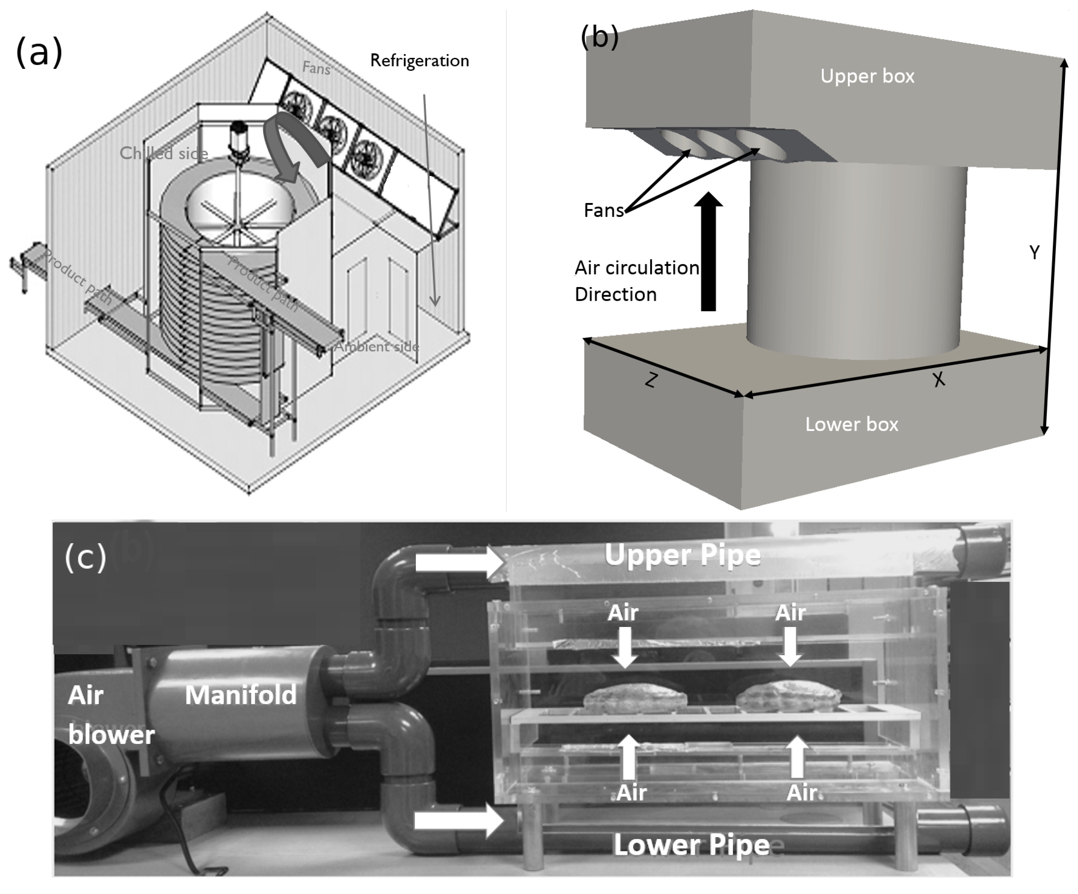
2. Industrial and Experimental Measurements

A schematic of the refrigeration spiral is shown in Figure 1a. The overall aim of the process is to cool the pasties from $85{}^{\circ }\mathrm{C}$ to less than $5{}^{\circ }\mathrm{C}$. This is done in two step; in the first step the product passes through an ambient environment for about 45 min before being moved into a chilled spiral for another 45 min. The spiral-cooling system comprises a large sealed environment with a refrigeration system built in and a spiral conveyor for moving products through at low speed. The spiral comprises 15 complete revolutions, with 360 pasties arranged on each tier (full revolution). The dimensions of the full refrigeration spiral are $8\mathrm{m}$ (X) ×$6\mathrm{m}$ (Y) ×$7\mathrm{m}$ (Z) as shown in Figure 1b. The spiral and fans are all contained within an enclosure with the fans used to circulate the air through the spiral from top to bottom with a return path outside the spiral within the enclosure. The evaporator for the refrigerator is usually installed in the bottom box of the spiral. After being chilled in the evaporator and recirculated, the air leaves the fans at temperature $-28{}^{\circ }\mathrm{C}$ and velocity $12\mathrm{m}/\mathrm{s}$. The diameter of each fan is $1.0\mathrm{m}$, so the three fans pump about $28{\mathrm{m}}^3/\mathrm{s}$ of chilled air around the system. In fluid dynamic terms, the fans raise the pressure in the upper box and decrease it in the lower box; thus forcing the air to make its way down across the mesh conveyor, cooling the product by removing the heat from its surface. In the computational model (see Section 4) this is represented by the domain in Figure 1b. with inlets (the fans) and outlet (the lower box).

In order to provide validation data for the CFD model of the complete spiral refrigeration unit, the air flow behavior inside the chilled spiral was measured at selected points using an $\Omega$ HHF1000 Series air velocity/temperature meter (temperature range $-40{}^{\circ }\mathrm{C}$ to $93{}^{\circ }\mathrm{C}$, velocity range 0 to $25.4\mathrm{m}/\mathrm{s}$, temperature accuracy $0.5\%$ full scale, velocity accuracy $1.5\%$ full scale). In order to further understand the cooling process, the temperature of individual pasties passing through the chiller was also monitored. To monitor the pasty temperature, six TMP36 Low Voltage temperature sensors (temperature range $-40{}^{\circ }\mathrm{C}$ to $125{}^{\circ }\mathrm{C}$, typical accuracy $\pm 1{}^{\circ }\mathrm{C}$ at $24{}^{\circ }\mathrm{C}$ and $\pm 2{}^{\circ }\mathrm{C}$ over complete temperature range) were inserted into the center of a fresh pasty, evenly distributed across the core region, and the pasty placed onto the conveyer. The sensors were connected to an Arduino for data logging, inside an insulated bag, and the maximum temperature recorded against time during the transit through the spiral chiller.

In addition, the cooling profile of a single Cornish pasty is also investigated. An experimental rig was developed for measuring the actual core temperature of a pasty, as shown in Figure 1c. The rig is made of two horizontal pipes, closed at one end but connected through a manifold to an air blower at the other end. The opposite sides of the pipes are connected to a rectangular box (dimensions: length $60\mathrm{cm}\times$ width $30\mathrm{cm}\times$ height $30\mathrm{cm}$) containing the pasties. The opposite faces of the pipes each have a slot ($2\mathrm{cm}\times 6\mathrm{cm}$) as an air outlet. The vertical distance between those slots is $13\mathrm{cm}$. The distance between the top pasty surface and the upper slot, and the bottom pasty surface and the lower slot is $4\mathrm{cm}$. The air blower pumps air into the pipes generating impinging jets of cold air onto both sides of the pasty with a velocity in the range of $15\mathrm{m}/\mathrm{s}$ to $20\mathrm{m}/\mathrm{s}$. A support structure made of metal wire is used in order to support the pasty. For measuring the temperature distribution inside the pasty, TMP36 temperature probes connected to an Arduino were used to store readings of the temperature inside the pasty. The experiment was run inside a freezer cabinet so that the air being circulated was at $-20{}^{\circ }\mathrm{C}$. As the bearing of the fan cannot sustain temperatures below about $-15{}^{\circ }\mathrm{C}$, it was necessary to keep the air blower running for 10 min outside of the freezer until the engine of fan reached about $40{}^{\circ }\mathrm{C}$. The implication of this process is that the air pumped from the fan takes about 10 min to reach the minimum temperature $-20{}^{\circ }\mathrm{C}$.

3. Mathematical and Physical Modelling

3.1. Governing Equations of Fluid Flow

The Navier-Stokes and heat transfer equations are used as mathematical models to solve for fluid flow and heat transfer during the cooling process. It is assumed that the flow is subsonic but the air is subject to thermal expansion, so the density is not constant. The equations are given as follows:

• Mass Conservation Equation

  $$\frac{\partial \rho }{\partial t}+\nabla .\mathbf{u}=0$$

  (1)
• Momentum Conservation Equation

  $$\frac{\partial \rho \mathbf{u}}{\partial t}+\mathbf{u}·\nabla \rho \mathbf{u}=-\nabla \mathbf{P}+\mu {\nabla }^2\mathbf{u}+\rho \mathbf{g}$$

  (2)
• The Heat Transfer Equation for a fluid is

  $$\rho C_{p.f}\frac{\partial T_f}{\partial t}+\rho C_{p,f}\mathbf{u}·\nabla T_f-k_f{\nabla }^2{T}_f=S_f$$

  (3)

Heat transfer in a solid is through conduction, and so the heat transfer equation for this is

$${\rho }_s{C}_p\frac{\partial T_s}{\partial t}=k_s{\nabla }^2{T}_s+S_s,$$

(4)

where $\rho$, $\mathbf{u}$, P, $\mu$, g are air density, velocity of flow field, pressure, dynamic viscosity and gravitational acceleration. $T_f$, $C_{p,f}$, $k_f$ and $S_f$ are: temperature, specific heat capacity and thermal conductivity of the fluid (i.e. the air) and the source term in the fluid field respectively. The parameters of the transport equation in solid respectively are: $T_s$, $k_s$, ${\rho }_s$ and $S_s$ are: the solid temperature, thermal conductivity, density of the solid and the source term in the solid domain. For simplicity it will be assumed that many of the coefficients (eg viscosity) do not vary with temperature, although this may not in fact be the case.

CFD simulation typically employs the Finite Volume methodology, in which the governing equations Equations (1)–(3) are discretised on a mesh comprising numerous individual control volumes or cells. Creating the mesh (or “meshing”) for any given geometry is a complex and challenging problem in its own right. The dependent variables P, $\mathbf{u}$ are represented by values stored at the cell centres, and the governing equations integrated over each individual cell to create a set of difference equations which can be solved implicitly through matrix inversion. Since this is a transient problem, it is solved using timestepping algorithms, PISO and Pimple; within each individual timestep these involve a “guess and correct” iterative procedure to deal with the intrinsic nonlinearity of the Navier Stokes equations. Various commercial and open source codes are available which implement these algorithms; in this work we use the commercial code ANSYS-Fluent and the open source code OpenFOAM.

3.2. Turbulence Modelling

The present problem includes forced air flow which generates convective heat transfer within the refrigeration system. The cooling fans blow the air at high velocity for which $Re=4\times {10}^6$. This suggests that the air flow is likely to be turbulent. The complex nature of turbulent flow means that direct simulation of all the components of the flow is only possible for very simple cases and never possible for complex real world cases. To overcome this, a turbulence model must be used; the equations of motion Equations (1)–(3) are averaged, using a process of ensemble or Reynolds averaging (generating the Reynolds Averaged Navier Stokes or RANS equations), and solved numerically using the same methodologies to calculate the mean flow patterns. The averaging process smooths out the turbulent component of the flow which must be replaced by a simpler statistical model or turbulence model. Commonly, these models solve for two variables, the turbulent kinetic energy k and a second variable which can be the dissipation rate $ϵ$ or the specific turbulence dissipation rate $\omega =ϵ/C_{\mu }k$ (or other variables, see [28] for more details). Here we will use the well-validated $k-\omega$–SST model for the purpose [29,30]. This is a two-equation eddy viscosity model which combines the $k-\omega$ model for the near-wall region and the standard $k-ϵ$ model for the far field, gaining the best elements of each model in doing so. Hence; the $\omega$ variable has good mathematical properties near the wall, and so the $k-\omega$ model can be integrated near-wall without recourse to a wall model. Since heat transfer from a surface is largely governed by boundary layer effects this is advantageous for our cases. However in the free stream the $k-\omega$ model is known to be sensitive to inlet boundary conditions, so the $k-\omega$–SST model switches to use the standard $k-ϵ$ formulation away from the wall. Both OpenFOAM and Fluent implement the $k-\omega$–SST model as a turbulence model option.

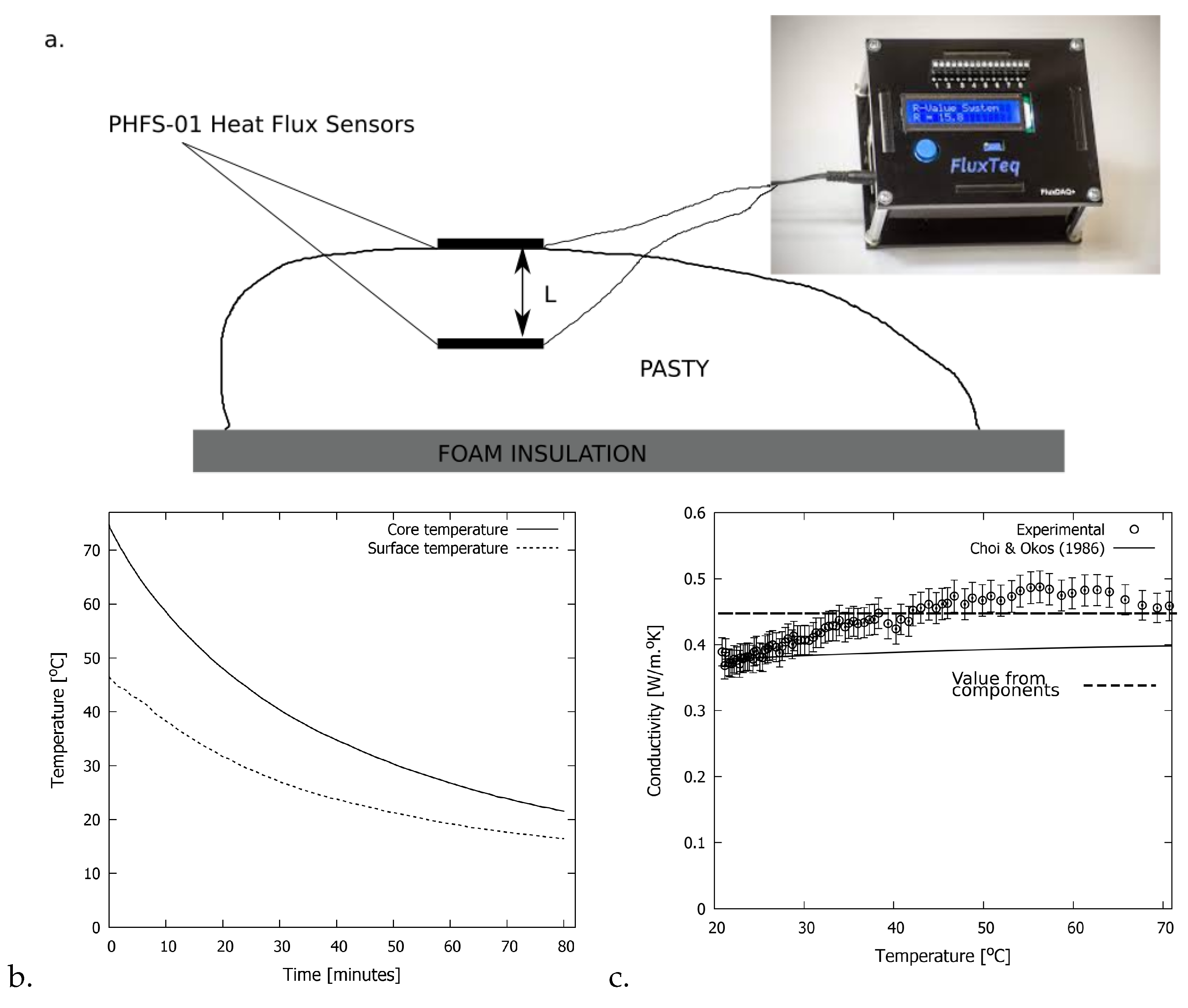
3.3. Thermal Properties of the Cornish Pasty

To complete the computational model, we need to determine the thermal properties of the different materials. The thermal properties of air are well known; however a Cornish Pasty is made of a number of separate food ingredients which differ in their thermal properties, so determining an exact value becomes very difficult [31], and there can be a considerable range in published values for any given food product [32]. In particular, for the calculations in Section 4.2.1 the pasty is treated as a homogeneous solid domain, for which we require a single set of thermodynamic coefficients representative of the mean properties. For the Cornish pasty, the density is obtained from the use of the ScanIP software (see below) to determine its volume, and the heat capacity can be determined experimentally [33]. However, determining the coefficient of thermal conductivity k is more complex. Based on analogy with electrical resistance, the mixture thermal conductivity can be calculated from the component thermal conductivities by considering them as a series of components in parallel

$$k=\sum _i{X}_i\times k_i$$

(5)

or in series

$$\frac{1}{k}=\sum _i\frac{X_i}{k_i}$$

(6)

where $X_i$ is the volume fraction of component ${}_i$ (determined from the mass fraction and density), and these different mixture thermal conductivities are recognised as predicting the upper and lower bounds of the thermal conductivities of most foods [34]. In the case of a pasty the filling is a jumbled mixture of components and so we have chosen to evaluate the system as a parallel system, recognising that this provides a plausible upper estimate of the value. The main pasty ingredients are beef mince, vegetables, liquids and pastry, and their thermophysical properties are available in the literature (see Ref [35]). The value of the conductivity coefficient determined this way is $k=0.47\mathrm{W}/\mathrm{m}\mathrm{K}$. However this figure is calculated for unbaked constituents at ambient temperature. Another option is to use the empirical equations proposed by Choi & Okos [6]. For heat conductivity, the coefficient is given as a function of temperature as follows:

$$k_p=1.7881\times {10}^{-1}+1.1958\times {10}^{-3}T-2.7178\times {10}^{-6}{T}^2$$

$$k_{fa}=1.8071\times {10}^{-1}-2.7604\times {10}^{-4}T-1.7749\times {10}^{-7}{T}^2$$

$$k_c=2.0141\times {10}^{-1}+1.3874\times {10}^{-3}T-4.3312\times {10}^{-6}{T}^2$$

$$k_{fi}=1.8331\times {10}^{-1}+1.2497\times {10}^{-3}T-3.1683\times {10}^{-6}{T}^2$$

$$k_a=3.2962\times {10}^{-1}+1.4011\times {10}^{-3}T-2.9069\times {10}^{-6}{T}^2$$

$$k_w=5.7109\times {10}^{-1}+1.7625\times {10}^{-3}T-6.7036\times {10}^{-6}{T}^2$$

where T is the temperature; and $k_p$, $k_{fa}$, $k_c$, $k_{fi}$, $k_a$ and $k_w$ are thermal conductivity of protein, fat, carbohydrate, fibre, ash and water respectively. These represent the primary components of the Cornish pasty, and their proportions in a typical Cornish Pasty [36] are given in

Table 1. Composition of processed Cornish Pasty

Name	Ratio %
water	47.3
Protein	7.0
Fat	17.8
Carbohydrate	24
Fibre	2.2
Ash	1.7

.

An alternative approach is simply to measure the various physical coefficients for a typical pasty. An experimental rig was set up to measure the coefficient of thermal conductivity by measuring temperature and heat flux from a cooling pastry (Figure 2a). FluxTeq PHFS-01 Heat Flux sensors were used; these are differential-temperature thermopile sensors each consisting of a square array of type T thermocouple sensors of size $2.5\times 2.5\mathrm{cm}$, giving a sensing area of $6.45{\mathrm{cm}}^2$ and thickness $0.38\mathrm{mm}$. Each sensor has a heat flux range of $\pm 150\mathrm{kW}/{\mathrm{m}}^2$ and an operating temperature range $-50{}^{\circ }\mathrm{C}$ to $+120{}^{\circ }\mathrm{C}$. The sensors were connected into a channel-in data reader through a set of cables. The data reader was then connected to a computer for storing the data. To get an appropriate reading of the heat flux and temperature, two sensors were attached to the bottom surface of the pasty whilst the third sensor was inserted inside the pasty. The bottom surface was used to avoid measuring through the air gap typically present in the top side of the pastry due to the cooking process; we were interested in measuring the heat transfer through solid filling and pastry. The pastry was placed upside down on an expanded foam board to minimise heat flux through the uninstrumented section of the pasty. To maximize the contact between the sensors and the surface of the pasty, a very thin layer of toothpaste was applied at the contact area. The distance between the two points of the core and surface was measured to be $L=2.5\mathrm{cm}$. The corresponding coefficient of thermal conductivity k was calculated using the solid heat conduction equation,

$$k=\frac{q\times L}{\Delta T},$$

(7)

assuming the measurement timescale is much shorter than the cooling timescale (around 80 minutes to cool from $70{}^{\circ }\mathrm{C}$ to room temperature). Here q is the measured heat flux, L is the distance between the measured temperature at the core of pasty $T_{in}$ of the pasty and its surface $T_{surface}$, and $\Delta T=T_{in}-T_{surface}$ is the temperature gradient between the inner and the surface of the pasty. Figure 2b shows the data for temperature for the Cornish pasty. The measurement was conducted at an ambient temperature below $5{}^{\circ }\mathrm{C}$. The temperature measured at the core and the surface of the pasty is presented in Figure 2b.

The values of thermal conductivity of Cornish pasty calculated using both Equation (7) and the various empirical methods are shown in Figure 2c. We recognise that all of these methods used to determine k have limitations, but are giving broadly similar values. The experimental values and those based on the empirical equations of Choi & Okos [6] both show some degree of temperature dependence; however this was felt to be within the range of uncertainty of the values and was ignored in the final computational model. Based on the above results and bearing in mind the temperature range of interest for the simulations (the pasty temperature is not expected to go below zero at any time), the coefficient of thermal conductivity for the current simulation is chosen as an average value $k=0.4\mathrm{W}/\mathrm{m}\mathrm{K}$. The finalised thermophysical properties of the Cornish pasty used in the numerical simulations are listed in

Table 2. Thermal properties of Cornish Pasty ($T>0{}^{\circ }\mathrm{C}$)

$\mathit{\rho }[\mathbf{kg}/{\mathbf{m}}^3]$	${\mathit{C}}_{\mathit{p}}[\mathbf{kJ}/\left(\mathbf{kg}\mathbf{K}\right)]$	$\mathit{k}[\mathbf{W}/(\mathbf{m}\mathbf{K}\left)\right]$
568	$3.3$	$0.40$

.

Where $\rho$, $C_p$ and k are the density, specific heat capacity and thermal conductivity of a Cornish pasty. The value of the density is calculated from the geometry of pasty generated using the ScanIP software, while the value of $C_p$ is already experimentally determined [33].

4. CFD Simulations

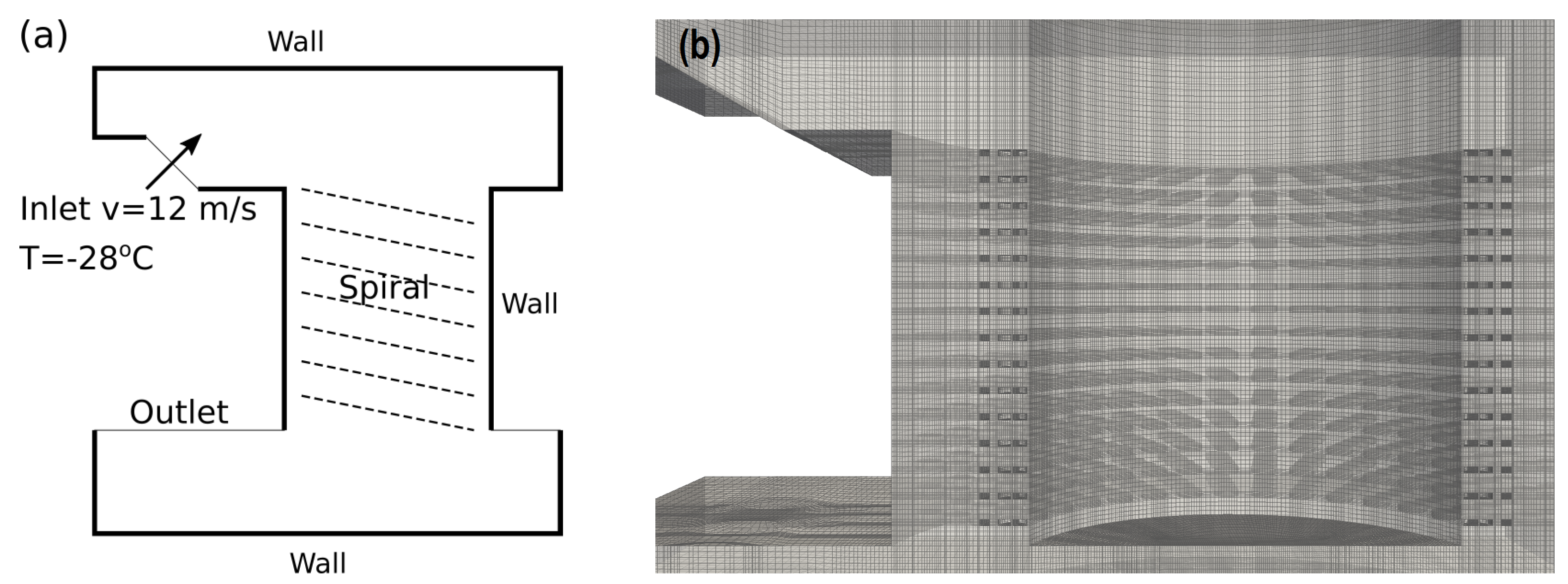
4.1. CFD Setup—Spiral Cooling System

The computational domain and the mesh used for conducting the simulation of the full spiral are presented in Figure 3. In reality the entire apparatus is enclosed in an enclosure with fans to circulate the air, but in the computational model this is represented by a single domain with inlets (the fans) and outlet (the base panel). The fans circulate about $28{\mathrm{m}}^3/\mathrm{s}$ of chilled air around the system; for the computational domain the fans are represented by fixed velocity inlets with inlet velocity $12\mathrm{m}/\mathrm{s}$ at a temperature of $-28{}^{\circ }\mathrm{C}$. For simplicity a standard D-shape is used to represent the pasties within the spiral, as the focus at this stage is understanding the air flow through the system. Since the starting and final temperatures for the pasties passing through the spiral are known, as is the time for them to travel through the system, the approximate temperature of a pasty at any location within the spiral can be approximated sufficiently well for the purpose of calculation of the air flow conditions throughout the system, and this was used to determine the boundary conditions for each individual pasty (fixed temperature boundary condition, with the temperature determined by the location within the spiral).

The open source code OpenFOAM (foam-extend-3.1) was used employing the $conjugateHeatFoam$ solver to solve the conjugate flow-field and heat transfer problem for predicting the cooling profile inside the spiral. The meshing tool Pointwise was used to generate the mesh. Meshes were generated with total cell counts of 10 million, 20 million and 70 million cells; results for 20 million and 70 million cells were found to be the same for the flow properties compared (velocities and temperatures at experimental locations; see Section 5.1), and so results in this paper are presented for the 20 million cell case. The mesh is clustered near the surface of the pasties for which $10>y^{+}>5$. An adjustable time step was used with an initial value of $\Delta t={10}^{-6}\mathrm{s}$ with the maximum Courant number (a non-dimensionalised representation of the timestep) set to 10 and the maximum time step was set to $\Delta t=0.01\mathrm{s}$. In order to maintain numerical stability, the standard numerical schemes for $conjugateHeatFoam$ have been adapted along with $limitedLinearValue0.33$ for the velocity and temperature advection terms. In addition, the coupled pressure-velocity equation was solved by employing the Pimple algorithm and the time marching was calculated with the implicit scheme $CrankNicolson0.5$. The properties of the air used in the current investigation are $1.225\mathrm{kg}/{\mathrm{m}}^3$ for density and kinematic viscosity $1.48\times {10}^{-5}{\mathrm{m}}^2/\mathrm{s}$. The results obtained for the spiral model are based on the setup of the boundary conditions in which the values of velocity and temperature are fixed and gravity is included in the y-direction. Both radiation and mass transfer are ignored as they do not significantly affect the heat transfer and the cooling profile.

4.2. CFD Setup – Single Cornish Pasty

To examine the detailed cooling process for the pasty, simulations have also been performed for the local air flow and heat transfer for a single pasty. This is obviously likely to be affected by the exact geometry of the pasty, and so Image Based Meshing (IBM) techniques have been employed. IBM was originally developed in the field of biomedical engineering and is used to generate meshes directly from medical scans produced using CT or MRI methods [37,38,39,40]. These scans provide 3d information about the inside of the patient in the form of regular spaced slices (2d images) which can be recombined to generate a voxelised (voxels are 3d pixels) representation of the internal structure, and this can be divided (segmented) into distinct computational regions representing blood vessels, bone, muscle etc. However the technique is widely applicable outside the medical area, and in particular can be used for reverse-engineering in any case where the geometry is complex and/or where no CAD model exists, but an example of the geometry is available for scanning [41,42]. In this case, MRI scans have been used to obtain the actual shape and internal structure of the pasty. Scanning was performed on a 1.5T Gyroscan magnet equipped with a Surface RF Coil (Philips, Amsterdam, The Netherlands) at the Exeter MR Research Centre. A 3-D T1-weighted Turbo Spin Echo (TSE) sequence was used (repetition time = $550\mathrm{ms}$, echo time = $14\mathrm{ms}$, flip angle $90{}^{\circ }$, field of view = $120\mathrm{mm}$, 65 transverse slices, $1\mathrm{mm}$ slice thickness and $1\mathrm{mm}\times 1\mathrm{mm}$ in plane resolution). This was then used as the basis of two separate simulations, as follows:

4.2.1. Localised Model, Homogeneous Pasty

The software package ScanIP (Synopsys Simpleware Software, Bradninch Hall, Castle St. Exeter EX4 3PL, UK) was used to convert the MRI scan into a CAD geometry for the surface of the pasty. This was exported to Pointwise and meshes created for the interior and exterior volumes as shown in Figure 4a. The interior was treated as a homogeneous solid with physical properties as determined in Section 3.3. Average values for the local air flow speed and temperature (determined from the simulation of the spiral cooling system by extracting values $5\mathrm{cm}$ above the pasties in the simulation) and used as boundary conditions for the simulation of the single pasty. Results from this model and comparison with experimental data taken from measurements of pasty temperatures in the industrial spiral itself and are shown in Section 5.1.

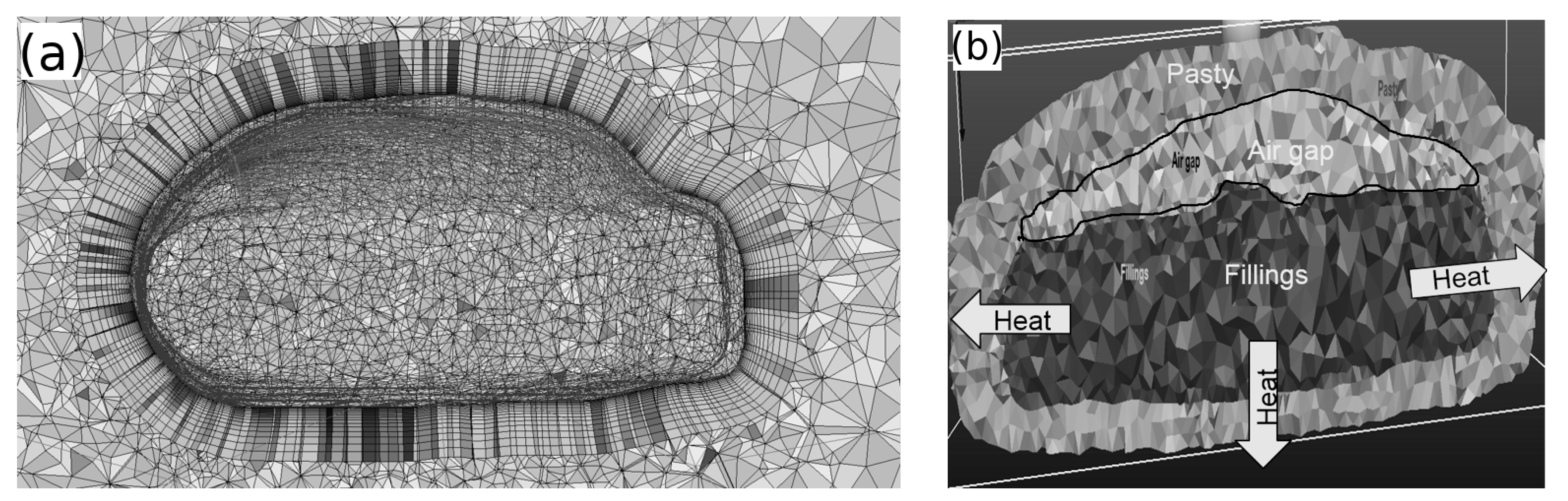
4.2.2. Localised Model, Resolved Pasty

The scan was segmented using the software ScanIP to identify the internal structure of the pastry, filling and the air gap (generated during cooking), generating separate meshed domains for these different components as shown in Figure 4b. Properties for the individual components (pastry, filling) were determined from literature. A separate experiment was performed to provide further experimental data for this case. The computational geometry was created to match this experiment, and results from this model and comparisons with the experimental results are shown in Section 5.3. Inlets at the top and bottom were set up to replicate the air jets in the real experiment. Coupled fluid and heat transfer calculations were performed to obtain the cooling profile, and for validation the results were compared against the experimental cooling profile. This allowed us to use CFD analysis to understand the actual effect of air velocity and temperature on the cooling process. For this simulation the conjugate heat transfer solver available in ANSYS-Fluent is used. As the interest is focused on the prediction of the heat extraction at the wall of the Cornish pasty, the mesh was generated ensuring a fine mesh at the thermal boundary layer meeting the condition $y{}^{+}$~1 at the interface of the fluid and the wall of the Cornish pasty. Whilst it is difficult to perform a mesh refinement study on IBM meshes (the geometry determined from the data and hence the mesh depends on the resolution of the scan, see [43] for details) the $y+$ values used indicates that the mesh is fine enough to resolve the physics of the heat transfer adequately in the boundary layer.

5. Results and Discussion

5.1. Spiral Cooling System

The experimentally measured speeds as registered by the HHF1000 anemometer as it travelled through the spiral are presented in Figure 5a. These measurements are registered in the centre of the conveyer belt $5\mathrm{cm}$ above the tops of the pastries. The distribution of the air velocity is not uniform at the upper tiers (first to third tier) so that at some points the velocity is higher but at other points the velocity is relatively low. At the lower tiers the distribution of the velocity across the conveyor becomes less variable. The peak values of the velocity shown on the curve correspond to the moment when the measuring device passes above one of the fans, which are installed about ~2 m below the conveyor so they blow the air up at an angle of $45{}^{\circ }$ to the horizontal towards the conveyor (the values of the velocity of air at these locations is the same as at the outlet of the fans).

The values of measured and numerically calculated velocities are averaged at each tier across the Right plane (see Figure 6a which identifies this plane in the geometry) and compared, the data is represented on Figure 5b. This clearly shows a good agreement between the measured and numerically calculated profiles, with an average discrepancy of $9.5\%$. The shape of the profiles are similar, although the simulation values are underpredicted. In the upper tiers the velocity is higher while at the lower tiers the velocity values decreased, levelling out at about $2\mathrm{m}/\mathrm{s}$. The difference in velocities must relate to the redistribution of flow across the spiral, and suggests that the cooling rate at the upper tiers is likely to be faster than for the lower tiers. Figure 5c,d show the time evolution of a representative pasty in transit through the system. Figure 5c shows the surface heat transfer coefficient; this is significantly affected by the air temperature and so shows an spike when the pasty is moved from the ambient to the chilled spiral. The temperature at the centre of the pasty was also monitored and the time variation compared with the calculated value in Figure 5d. Again, the profiles agree very well, although with some discrepancy beyond 70 min. This may be related to the thermodynamic coefficients (heat conduction coefficient etc) being taken to be constant rather than varying with the declining temperature. The desired target temperature of $5{}^{\circ }\mathrm{C}$ is marked on the graph.

Figure 6 demonstrates the pasties’ distribution across the conveyor and the streamlines that illustrate the air pattern inside the chiller spiral. At the upper tiers the pasties are warm (red color) but by reaching the lower tier the core’s temperature of pasties has dropped below $5{}^{\circ }\mathrm{C}$ (blue color) as Figure 6a shows. The behavior of the air flow within the spiral is described by the streamlines shown in Figure 6b. The flow is turbulent at the top and bottom boxes but at the level of the conveyor, which is confined between the belt and drum, the streamlines are more lined up and concentrated across the meshed conveyor. The behaviour of the flow can be more clearly seen by examining the linked animation Line2Spiral155.avi provided as a supplimentary animation file. The simulation for this animation was performed on the finest mesh (70 million cells) and shows the full time resolved behaviour of the flow.

5.2. Individual Cooling; Homogeneous Pasty

The model described in Section 5.1 concentrates on describing the air flow around the multiple pasties inside the spiral chiller. The energy equation is solved for the air domain only, and the surface temperatures of the individual pasties are fixed. This temperature record was then compared with results from the CFD model described in Section 4.2.1, which models the conjugate heat transfer problem of a single homogeneous pasty cooling in air. Boundary conditions for the local environment were based on averaged values extracted from just above the pasties in the spiral model.

The typical heat transfer coefficient (HTC) values at the Cornish pasty surface and the cooling profile of the pasty during whole cooling process, which includes ambient and chilled side, are shown in Figure 5c–d. The curve of Figure 5c illustrates the cooling process through heat extraction at different locations while traveling on the conveyor within the ambient and chiller sides. In the ambient spiral there is no forced circulation and so cooling is purely driven by buoyancy effects. Therefore, the heat extraction is purely influenced by the large gradient in temperature between the pasty and the surrounding air. Therefore, the heat extraction rate is expected to be low when the conveyor is intensively populated with Cornish pasties. In addition to this, the ambient air remains confined in the vicinity of the pasties between the drum and the belt, which leads to an increase in the air temperature because of heat accumulation in the ambient side. In the chiller side, the heat extraction is increased significantly due to the forced convection, in particular in the top tiers where the velocity of the air is relatively higher. Reduction in the HTC at the lower tiers can be explained by two factors. In addition to the drop in the velocity of the air, the difference in temperature inside and outside of the pasty also affects the heat removal from the surface of the pasty. Figure 5d represents the corresponding cooling profile of a Cornish pasty where both the measured and and numerically calculated profiles are compared. The numerical data are obtained by using the inlet boundary conditions from the data of measured air velocity presented in Figure 5b. As Figure 5c illustrates, the numerical prediction of the cooling profile is in good agreement with the measured values. However, differences between the experimental and numerical results become apparent when approaching the freezing point. To capture more accurate results, there would be a need to measure the actual thermo-physical properties of the Cornish pasty near and below the freezing point, which is out of the scope of the current study. In addition too, the cooling rate is plausibly affected by the internal pasty configuration. It is a difficult task to numerically capture effectively the poor compactness of the filling and air gaps which increase the thermal resistance to the heat flux from the core of the pasty to the surroundings, but this is the subject of the next section.

5.3. Local Cooling Processes

An equivalent numerical simulation has been conducted using a realistic geometry for the Cornish pasty which is shown on Figure 7a, developed using the Image Based Meshing methods described in Section 4.2. Figure 7c. depicts the flow impinging on the top and bottom surfaces of the pasty. The flow is uniform at the top and bottom surfaces wrapping the pasty but at the intersection of upper and lower air jets the air recirculation develops close to the wall pasty. Figure 7d. presents the comparison between numerical and experimental core temperatures for the pasty evolving over time. The numerical data was obtained using average velocity and temperature averaged values of chilled air. The air velocity was $18.5\mathrm{m}/\mathrm{s}$ and the temperature was $T=-1{}^{\circ }\mathrm{C}$ in the first 10 min and $T=-21{}^{\circ }\mathrm{C}$ in the rest of the simulation. Overall the results show a good match between the numerical and experimental results. The slight divergence of the simulation curve at the late time of cooling is due to the fact that the thermophysical properties of the pasty become heavily dependent on the temperature at lower temperatures.

Figure 8a,b show the distribution of the temperature in two different planes cut horizontally and vertically at the core point of the pasty. Figure 8c,d depict the corresponding profiles of temperature at the lines crossing the region of high temperature on the contours. Interestingly, one may note that where there is no air gap, the cooling uniformly progresses from the surface of the pasty towards the core body of pasty as indicated in Figure 8a,c. Therefore, the temperature profile is almost symmetric; the heat is extracted with the same rate at both sides of the pasty. Figure 8b,d demonstrate the effect of a thin air gap between the upper surface and the filling. The cooling rate at the bottom surface is faster than at the upper surface and so the higher temperature region is concentrated near to the upper surface (Figure 8b). The temperature profile is not symmetric as Figure 8d indicates, the peak value of the temperature being shifted towards the location of the air gap at the upper side of the pasty. Above the air gap, the temperature profile is varying linearly similar to the case of a wall separated by two fluid regions with different temperatures. These results predict that the heat extraction is more efficient at the bottom and side surfaces of the pasty.

6. Conclusions

In the present study CFD simulations have been conducted to investigate the industrial cooling of a specific food product (Cornish pasties). An initial experiment was conducted to determine the thermal conductivity of the pasty, which was used with the already determined thermophysical properties for the subsequent CFD simulations. Three sets of CFD simulations were carried out, as follows:

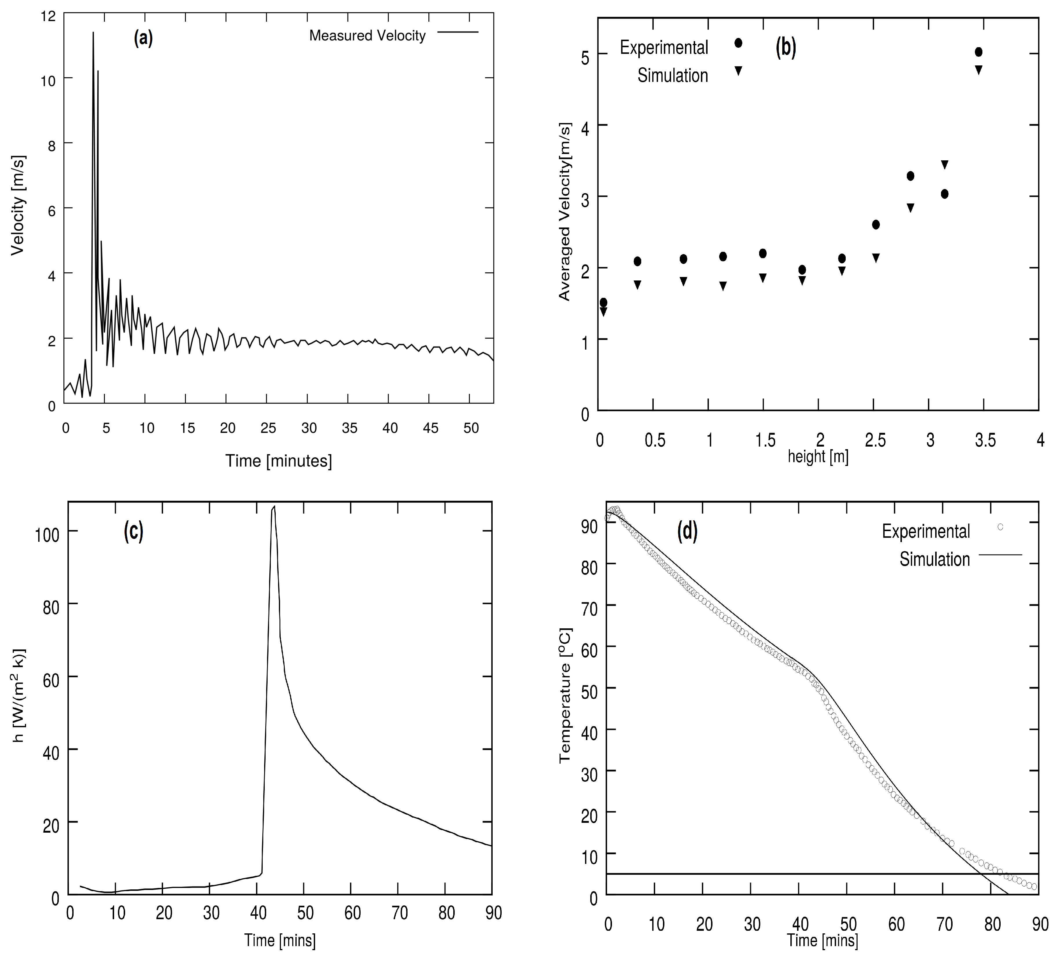
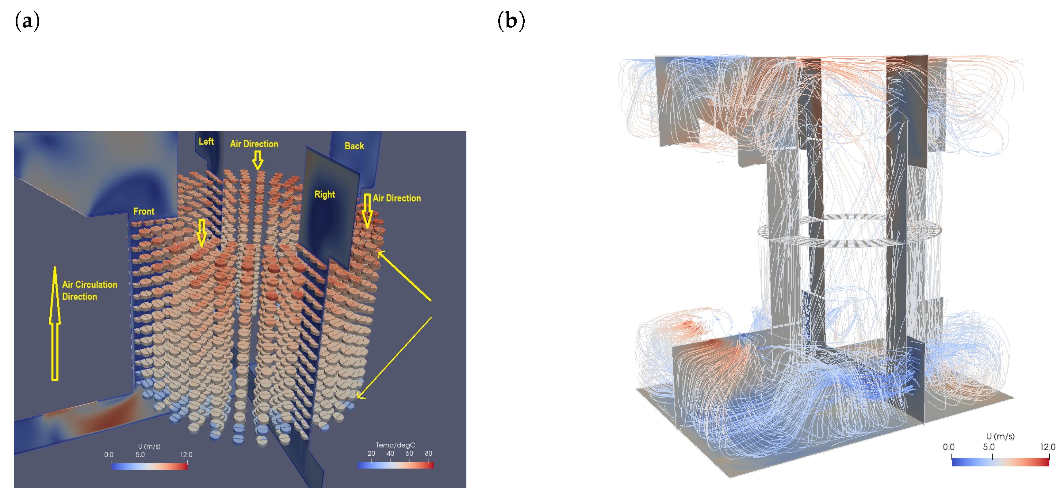
• A full simulation of a spiral chiller. This represented the individual pasties as D-shaped blocks at fixed temperatures, with 360 pasties in each $360{}^{\circ }$ revolution (the spiral containing 15 complete turns), and focussed on the thermofluid simulation of the air through the equipment. Results were compared and validated against air flow data measured in the actual industrial spiral.
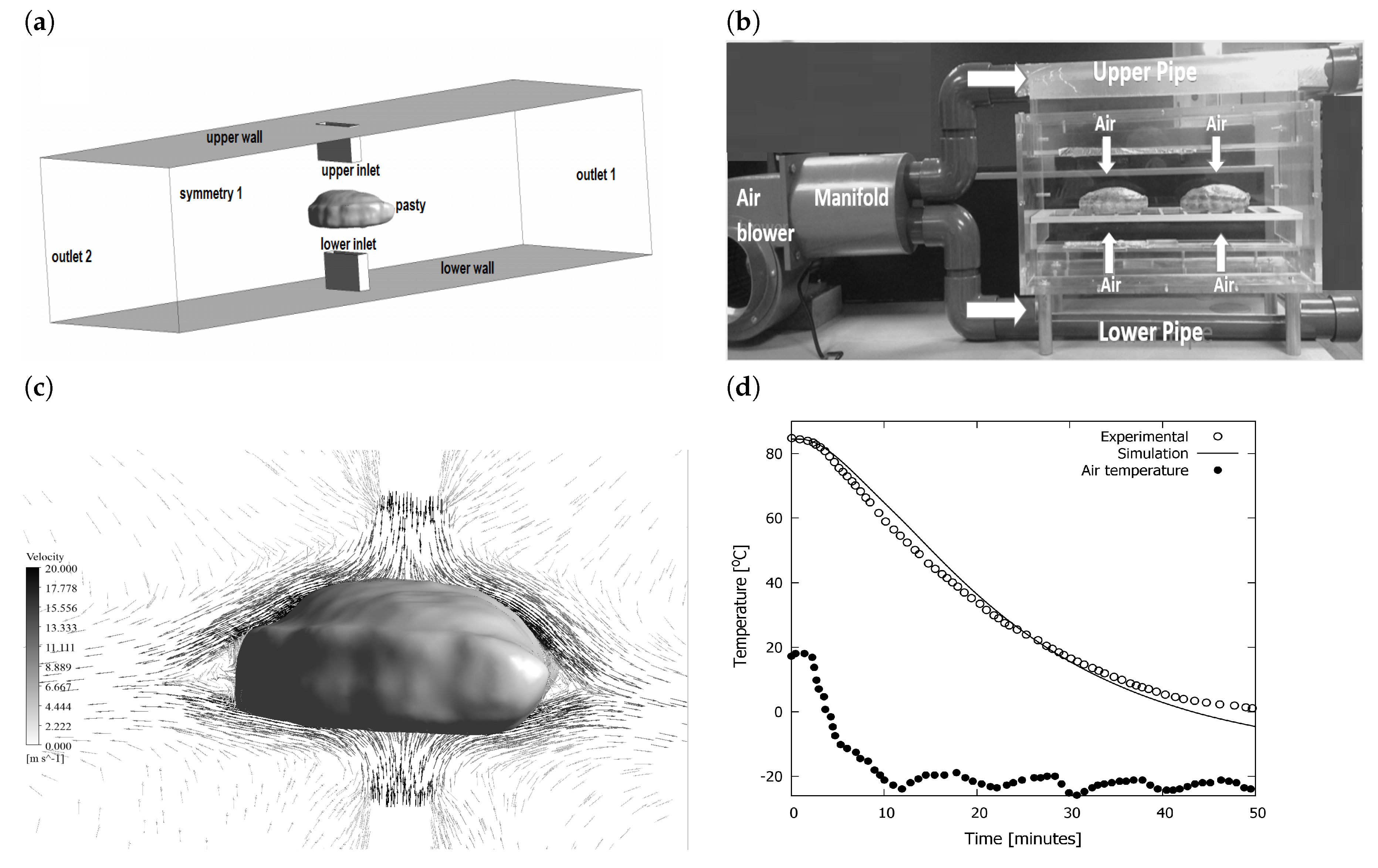
• A Conjugate Heat Transfer simulation of an individual, isolated pastry. This used MRI scans to determine the external geometry of the pastry, which was then represented as a single homogeneous solid region cooling via heat transfer to the surrounding air. The air boundary conditions were based on data extracted from the first simulation of the full spiral. Results from these simulations were compared with time series temperature data recorded in individual pasties travelling through the system.
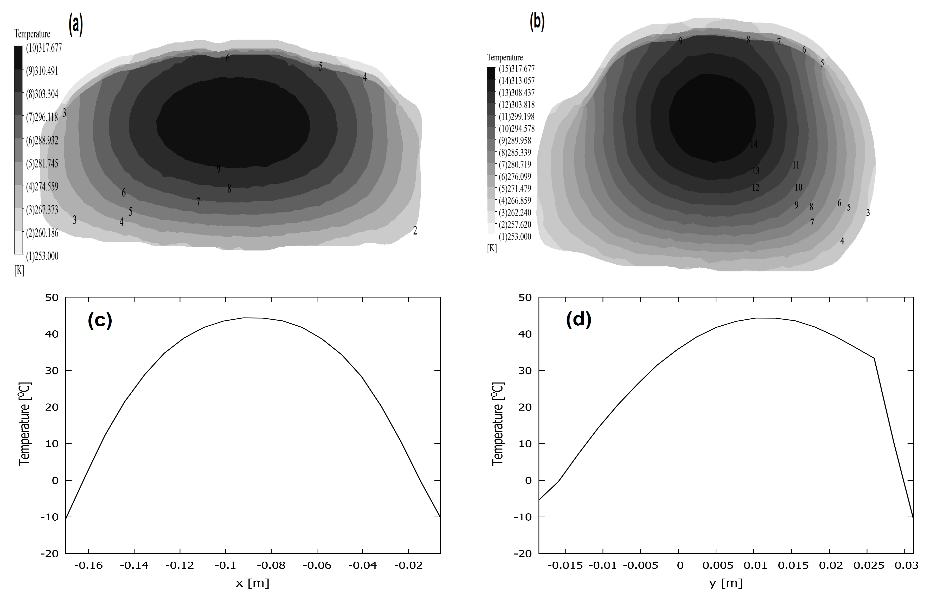
• A third set of simulations was carried out in which the interior structure of an individual pasty was resolved using Image Based Meshing (IBM) techniques. MRI scans of the pasty were segmented using ScanIP to provide separate domains for air, pastry, filling and air gap. A full simulation of the cooling and heat transfer was then performed. This model matched a separate experiment in which individual pasties were cooled by the impact of jets of cold air, and the results from the experiment and CFD were compared.

Very close agreement was found between the results from the CFD simulations and the equivalent experimental data, both captured from measurements made in the industrial system and for the isolated experiment. Whilst the interior structure and thermophysical properties of the pasties is complex, simplifying assumptions (such as constant values for k) can be made in order to make the problem computationally tractable. Numerical simulations are always a process of approximation, and our results demonstrate that even where we have made significant approximations the results correlate well enough with measurements to give confidence in the results. Predictions of the overall thermofluid dynamics in the spiral system can be reliably made using CFD, even with such a large number of pasties within the spiral, whilst the cooling of the individual pasties can also be reliably predicted. Such calculations could in future be used to optimise the system and/or process operation of the cooling spiral, for instance to reduce the carbon footprint of this energy-intensive operational process by exploring its cooling behaviour under a range of different input paramters. Given the computational cost of running individual simulations, this is likely to involve the construction of a surrogate model, tuned on a limited number of computational runs and able to interpolate the results to predict the results for any combination of input parameters. We have also demonstrated the ability of IBM to construct a detailed model of the interior structure of a pasty.

References

1. Hung, Y.; Thompson, D. Freezing time prediction for slab shape foodstuffs by an improved analytical method. J. Food Sci. 1983, 48, 555–560. [Google Scholar] [CrossRef]
2. Gaffney, J.J.; Baird, C.D.; Chau, K.V. Method for calculating heat and mass transfer in fruits and vegetables individually and in bulk. ASHRAE Trans. 1985, 91, 332–352. [Google Scholar]
3. Hossain, M.; Cleland, D.; Cleland, A. Prediction of freezing and thawing times for foods of three-dimensional irregular shape by using a semi-analytical geometric factor. Int. J. Refrig. 1992, 15, 241–246. [Google Scholar] [CrossRef]
4. Dincer, I. Methodology to determine temperature distributions in cylindrical products exposed to hydrocooling. Int. Commer. Heat Mass Transf. 1993, 19, 359–371. [Google Scholar] [CrossRef]
5. Carroll, N.; Mohtar, R.; Segerlind, L.J. Predicting the cooling time for irregular shaped food products. J. Food Process. Eng. 1996, 19, 385–401. [Google Scholar] [CrossRef]
6. Choi, Y.; Okos, M.R. Effects of temperature and composition on the thermal properties of foods. In Food Engineering and Process Applications; Elsevier Applied Science: London, UK, 1986; Volume 1, pp. 93–101. [Google Scholar]
7. Kaale, L.D.; Eikevik, T.M.; Kolsaker, K. Superchilling of food: A review. J. Food Eng. 2011, 107, 141–146. [Google Scholar] [CrossRef]
8. Salvadori, V.; Mascheroni, R. Analysis of impingement freezers performance. J. Food Eng. 2002, 54, 133–140. [Google Scholar] [CrossRef]
9. Midden, T.M. Impingement air baking for snack foods. Cereal Foods World 1995, 40, 532–535. [Google Scholar]
10. Acosta, J.L.; Moreira, R.G.; Yagoobi, J.S. Air impingement drying of tortilla chips. Dry. Technol. 1997, 15, 881–897. [Google Scholar]
11. Nitin, N.; Karwe, M.V. Heat transfer coefficient for cookie shaped objects in a hot air jet impingement oven. J. Food Process. Eng. 2001, 24, 51–69. [Google Scholar] [CrossRef]
12. Erdogdu, F.; Sarkar, A.; Singh, R.P. Mathematical modeling of air-impingement cooling of finite slab shaped objects and effect of spatial variation of heat transfer coefficient. J. Food Eng. 2005, 71, 287–294. [Google Scholar] [CrossRef]
13. Wahlby, U.; Skjoldebrand, C.; Junker, E. Impact of impingement on cooking time and food quality. J. Food Eng. 2000, 43, 179–187. [Google Scholar] [CrossRef]
14. Sarkar, A.; Singh, R.P. Spatial variation of heat transfer coefficient in air impingement applications. J. Food Sci. 2003, 68, 910–916. [Google Scholar] [CrossRef]
15. Smale, N.; Moureh, J.; Cortella, G. A review of numerical models of airflow in refrigerated food applications. Int. J. Refrig. 2006, 29, 911–930. [Google Scholar] [CrossRef]
16. Hoang, M.; Verboven, P.; Baerdemaeker, J.D.; Nicolaï, B. Analysis of the air flow in a cold store by means of computational fluid dynamics. Int. J. Refrig. 2000, 23, 127–140. [Google Scholar] [CrossRef]
17. Rouaud, O.; Havet, M. Computation of the airflow in a pilot scale clean room using K-ϵ turbulence models. Int. J. Refrig. 2002, 25, 351–361. [Google Scholar] [CrossRef]
18. Nahor, H.; Hoang, M.; Verboven, P.; Baelmans, M.; Nicolaı, B. CFD model of the airflow, heat and mass transfer in cool stores. Int. J. Refrig. 2005, 28, 368–380. [Google Scholar] [CrossRef]
19. Foster, A.; Swain, M.; Barrett, R.; James, S. Experimental verification of analytical and CFD predictions of infiltration through cold store entrances. Int. J. Refrig. 2003, 26, 918–925. [Google Scholar] [CrossRef] [Green Version]
20. Huan, Z.; Ma, Y.; He, S. Airflow blockage and guide technology on energy saving for spiral quick-freezer. Int. J. Refrig. 2003, 26, 644–651. [Google Scholar] [CrossRef]
21. Chanteloup, V.; Mirade, P.S. Computational fluid dynamics (CFD) modelling of local mean age of air distribution in forced-ventilation food plants. J. Food Engng. 2009, 90, 90–103. [Google Scholar] [CrossRef]
22. Mirade, P.S. Prediction of the air velocity field in modern meat dryers using unsteady computational fluid dynamics (CFD) models. J. Food Eng. 2003, 60, 41–48. [Google Scholar] [CrossRef]
23. Kuffi, K.D.; Defraeye, T.; Nicolai, B.M.; Smet, S.D.; Geeraerd, A.; Verboven, P. CFD modeling of industrial cooling of large beef carcasses. Int. J. Refrig. 2016, 69, 324–339. [Google Scholar] [CrossRef]
24. Cortella, G.; Manzan, M.; Comini, G. CFD simulation of refrigerated display cabinets. Int. J. Refrig. 2001, 24, 250–260. [Google Scholar] [CrossRef]
25. D’Agaro, P.; Cortella, G.; Croce, G. Two- and three-dimensional CFD applied to vertical display cabinets simulation. Int. J. Refrig. 2006, 29, 178–190. [Google Scholar] [CrossRef]
26. Rossetti, A.; Minetto, S.; Marinetti, S. A simplified thermal CFD approach to fins and tube heat exchanger: Application to maldistributed airflow on an open display cabinet. Int. J. Refrig. 2015, 57, 208–215. [Google Scholar] [CrossRef]
27. Alfaro-Ayala, J.A.; Uribe-Ramirez, A.R.; Minchaca-Mojica, J.I.; de, J.; Ramírez-Minguela, J.; Alvarado-Alcalá, B.U.; López-Nëz, O.A. Numerical prediction of the unsteady temperature distribution in a cooling cabinet. Int. J. Refrig. 2017, 73, 235–245. [Google Scholar] [CrossRef]
28. Jiang, L.; Tabor, G.; Gao, G. A new turbulence model for separated flows. Int. J. Comput. Fluid Dyn. 2011, 25, 427–438. [Google Scholar] [CrossRef]
29. Menter, F. Two-Equation Eddy-Viscosity Turbulence Models for Engineering Applications. AIAA J. 1994, 32, 1598–1605. [Google Scholar] [CrossRef]
30. Menter, F.; Esch, T. Elements of industrial heat transfer prediction. In Proceedings of the 16th Brazilian Congress of Mechanical Engineering (COBEM), Minas Gerais, Brazil, 26 November 2001. [Google Scholar]
31. Carson, J.K. Thermal Conductivity Measurement and Prediction of Particulate Foods. Int. J. Food Prop. 2015, 18, 2840–2849. [Google Scholar] [CrossRef]
32. Carson, J.K. Measurement and Modelling of Thermal Conductivity of Sponge and Yellow Cakes as a Function of Porosity. Int. J. Food Prop. 2014, 17, 1254–1263. [Google Scholar] [CrossRef]
33. Rodriguez, R.; Rodrigo, M.; Kelly, P. A Calorimetric Method To Determine Specific Heat of Prepared Foods. J. Food Eng. 1995, 26, 81–96. [Google Scholar] [CrossRef]
34. Murakami, E.G.; Okos, M.R. Measurement and prediction of thermal properties of foods. In Food Properties and Computer-Aided Engineering of Food Processing Systems; Singh, R.P., Medina, A.G., Eds.; Kluwer Academic: Dordrecht, The Netherlands, 1989; pp. 3–48. [Google Scholar]
35. Owen, M.S. (Ed.) ASHRAE Handbook: Refrigeration Systems and Applications; American Society of Heating, Refrigerating and Air Conditioning Engineers: Atlanta, GA, USA, 1986. [Google Scholar]
36. Roe, M.; Church, S.; Pinchen, H.; Finglas, P. Nutrient Analysis of a Range of Processed Foods with Particular Reference to Trans Fatty Acids; Technical report; Institute of Food Research, Institute of Food Research, Norwich Research Park: Colney, UK, 2013. [Google Scholar]
37. Weber, I.; Young, P.G. Automating the generation of 3D finite element models based on medical imaging data: application to head impact. In Proceedings of the 2D Modelling, Paris, France, 23–24 April 2003. [Google Scholar]
38. Xuan, V.B.; Weber, I.; Füreder, R.; West, T.B.; Young, P.G. Automating the Generation of Finite Element Models based on 3D data: Generation of a mesh for CFD analysis of the trachea. In Proceedings of the 6th International Symposium on Computer Methods in Biomechanics and Biomedical Engineering, Madrid, Spain, 25–28 February 2004. [Google Scholar]
39. Collins, T.P.; Tabor, G.R.; Young, P.G. A computational fluid dynamics study of inspiratory flow in orotracheal geometries. Med. Biol. Eng. Comput. 2007, 45, 829–836. [Google Scholar] [CrossRef] [PubMed]
40. Young, P.; Beresford-West, T.; Murphy, F. Imaged based meshing and its role within computational biomechnics. In Proceedings of the International Biomechanics Conference, Ottowa, ON, Canada, 2–6 June 2008. [Google Scholar]
41. Tabor, G.; Xuan, B.; Füreder, R.; West, T.; Young, P.G. On Automating the Generation of CFD Models Based on 3D Data: Industrial and Biomedical Applications. In Proceedings of the ECCOMAS Congress, Jyvaskyla, Finland, 24–28 July 2004. [Google Scholar]
42. Tabor, G.; Young, P.G.; West, T.B.; Benattayallah, A. Mesh construction from medical imaging for multiphysics simulation: Heat transfer and fluid flow in complex geometries. Eng. Appl. Comput. Fluid Mech. 2007, 1, 126–135. [Google Scholar] [CrossRef]
43. Baker, M.; Young, P.; Tabor, G.R. Image based meshing of packed beds of cylinders at low aspect ratios using 3d MRI coupled with computational fluid dynamics. Comput. Chem. Eng. 2011, 35, 1969–1977. [Google Scholar] [CrossRef]
Figure 1. Experimental setups to measure data for validation comparison. (a) shows a schematic of the air flow domain for the refrigeration spiral. The spiral comprises 15 complete revolutions, with 360 pasties are arranged on each tier (full revolution). The overall height of the spiral is 6 m. (b) shows the air flow domain as simulated in CFD. (c) shows a photograph of the experimental rig developed for measuring the core temperature of a singe pasty.
Energies 12 03358 g001
Figure 2. Experimental measurement of the thermal coefficient k for a representative pasty. (a) shows a schematic representation of the experimental setup with PHFS-01 Heat Flux sensors inserted at the centre and surface of the pasty. Data in (b) represents the temperature profiles at the core and the surface of the Cornish pasty, the distance between the core and surface being 2.5 cm . Data in (c) shows the experimental and empirical values of the heat conductivity coefficient of the Cornish pasty. Error bars in the experimental measurements have been estimated from measurement errors for the different input parameters.
Energies 12 03358 g002
Figure 3. (a) Schematic of the computational domain for the full industrial spiral, and (b) structured mesh of the interior of the domain. The spiral comprises 15 complete revolutions, whilst 360 pasties are arranged on each tier (full revolution). The overall height of the spiral is 6 m .
Energies 12 03358 g003
Figure 4. (a) shows a slice through the homogeneous pastry model divided into interior (solid) and exterior (air) regions. This demonstrates the clustered mesh around the pasty, where the mesh is very fine across the boundary layer ( y + ~1) to accurately calculate the conjugate heat transfer. (b) shows the segmented scan for the resolved pasty dividing the interior into pastry, filling and air gap.
Energies 12 03358 g004
Figure 5. Data in (a) represents the measured velocity profile inside chiller spiral, the values of the velocity were measured from the upper tier to the lower tier (as shown in Figure 6a) across the chilled spiral. Data in (b) represents the average-velocity at each tier compared with the measured velocity at each tier. Data in (c) represents the heat transfer coefficient at the surface of a representative Cornish pasty obtained in ambient and chilled side. Data in (d) presents the measured and simulated temperature profiles at the core of pasty across whole cooling time in ambient and chilled sides.
Energies 12 03358 g005
Figure 6. Flow field pattern visualization in the spiral for (a) the pasties distributed in the spiral and (b) the Streamlines which illustrate air flow behavior inside the spiral system. In (a) the surface temperature of the pasties is indicated by the right hand colour map; the flow speed on the cutting planes by the left hand colour ma; the same colour map being used on the streamlines for figure (b).
Energies 12 03358 g006
Figure 7. Computational simulation of the cooling of a single Cornish pasty. (a) demonstrates the overall computational domain which closely matches the experiment. (b) shows the equivalent experiment whilst (c,d) show results from the simulation for air flow and core temperature; the latter being compared with the actual measured results.
Energies 12 03358 g007
Figure 8. (a,b) represent the temperature contours across the length and width planes respectively, the numbers on the contours are referring to the values of the temperature on the legend. (c,d) represent the temperature profiles at horizontal in x-direction (length of pasty is 186 cm ) and vertical in y-direction (the thickness of pasty is 5.1 cm ) lines crossing the region of high temperature on the contours.
Energies 12 03358 g008