1. Introduction
In Japan, power-related administrative reforms have been progressing since the 2011 earthquake. The liberalization of the electricity market is a major pillar of this policy. From the ministry of economy, trade and industry (METI) report [
1], until now, the power market has been monopolized by regional corporations, and a single large power company has provided almost all of the power in a given region. The Tokyo Electric Power Company, which caused a nuclear accident, is one such company. The public reaction on the accident has led to a demand for a system that will allow consumers to select a preferred power company. In fact, the liberalization of electricity retail began in 2016, and it is expected to continue being liberalized going forward.
The Japanese government is promoting the liberalization of electricity concurrently with the introduction of renewable energy; furthermore, it is trying to promote power trading through one market player, namely the Japan Electric Power Exchange (JEPX). In the spot market, all bids are matched every 30 min; thus, 48 products are traded every 30 min per day. The minimum volume that can be traded during a 30-min bid is 1 MW (equivalent to 500 kWh). The bid supply and demand are matched by using the price auction method. In the case of congestion of electricity, the exchange is split by a regional hub, and the transaction is carried out in each split market. When there is no intersection between the supply and demand caused by oversupply, the spot price is deemed to be zero (see JEPX website [
2]).
However, as we explain in
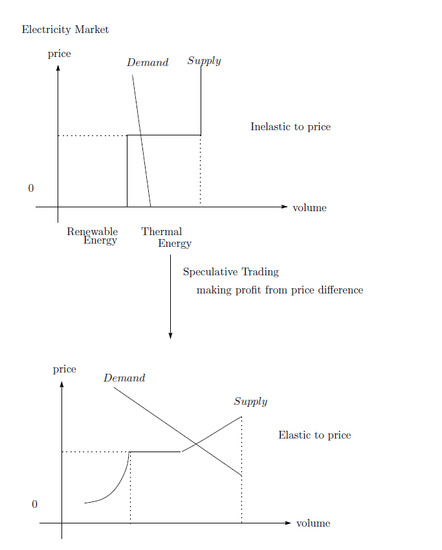
Section 3, the electricity market possesses some special properties (such as demand price-in-elasticity and merit order curve) that are different from the normal goods handled in economics. For this reason, electric power industries in regions such as Europe also supplement the electricity market through various mechanisms. The forward market (that is, the opening up of an electricity market before electric power is actually supplied) is one of the mechanisms for increasing the liquidity of electric power.
Of course, the forward market has already been opened by using JEPX. There are four types of forward products, including monthly 24-h products, weekly 24-h products, monthly daytime products, and weekly daytime products. Bid supply and demand is matched through continuous sessions.
The development of forward markets is also important from the perspective of renewable energy propagation. The growing popularity of renewable energy is, of course, a natural consequence of nuclear power plant accidents. Nuclear power has a lower environmental impact compared to thermal power, and it has been introduced for that purpose in Japan. Furthermore, the policy for cleaner renewable energy achieved national attention after the earthquake. However, renewable energy is produce through a variable energy system in which the amount of power generation is affected by various environmental factors such as sunshine hours, wind speed, and rainfall. Because weather information changes from moment to moment, the existence of markets with various timelines that correspond to such information is also essential for considering business operator’s risk aversion.
Previous research has pointed out that increasing the liquidity of renewable energy is also an important factor in the penetration of renewable energy; thus, based on this aspect as well, the forwards market is an essential system. For example, researchers investigating wind power generation in Germany pointed out the importance of increasing the liquidity of electricity (Holttinen (2005) [
3], Ummels et al. (2006)) [
4]. Markets with several timelines raise the liquidity of electricity and it becomes easy to trade electricity produced by renewable energy.
However, increasing the amount of trading opportunities includes one other aspect: allowing market participants to dynamically perform speculative actions. Electric power is difficult to save, but if the liquidity of the market increases, and the electricity transaction becomes easier, it is natural that some market players make profits by using price differences. In this paper, we use a simple model based on JEPX to analyze the speculative behavior in the dynamic power market. Moreover, we show that the demand inelasticity is improved by the speculative trading. The inelasticity of demand in the electricity market is well known, and it is one of the causes of inefficiencies, such as price manipulation by suppliers. However, our findings show that speculative action may improve the inelasticity and increase market welfare. Our model is based on JEPX; however, the basic factor of the model is not specific to Japan. This model can be applied as a more general model in electricity markets.
The rest of the paper is organized as follows.
Section 2 introduces related literature, and
Section 3 explains the standard electricity market features.
Section 4 then introduces the heterogeneous belief model, and it includes many of the electricity market features noted in
Section 3.
Section 5 presents the theoretical results and discusses some policy implications. Finally,
Section 6 provides some concluding remarks.
2. Related Literature
Following the full-scale liberalization of electricity retailing, constructing forward market has become an urgent agenda for the further vitalization of the electricity wholesale market, which is an important source of power procurement for electricity retailers. It is crucial to develop an electricity forwards market that can effectively aid the formation of fair and transparent price indicators and help to hedge against the risk of fluctuations in electricity wholesale prices.
Lucia et al. (2002) [
5] and Pilipovic (1998) [
6] examined the importance of the regular pattern in the behavior of electricity prices and its implications for the purposes of forward pricing. Other empirical papers, such as those by Escribano et al. (2002) [
7], Eydeland et al. (2003) [
8], Huisman et al. (2003) [
9], and Maekawa et al. (2018) [
10], have introduced a panel model for determining hourly electricity prices in forward markets and thus examined their characteristics. These models consider several factors: seasonality, regime switching, or price spikes.
Research in this field has been actively conducted recently. For example, Botterud et al. (2010) [
11] analyzed 11 years of historical spot and forward prices from the hydro-dominated electricity market and found that forward prices tended to be higher than spot prices.
By using multivariate models, Raviv et al. (2015) [
12] demonstrated that the disaggregated hourly prices contained useful predictive information of the daily average price in the Nord Pool market.
All these papers utilized an empirical perspective. However, to understand the relationship between spot prices and forward prices, it is essential to construct a microeconomic theoretical model. The power market has many special conditions, and it is difficult to simply adopt any particular economic point of view.
In response to these empirical studies, power market prices are being modeled in many studies. There is a long list of papers for wholesale power prices and electricity derivatives (e.g., Cartea et al. (2005) [
13], Weron (2007) [
14], Hikspoors et al. (2007) [
15], Benth et al. (2008) [
16], and Jaimungal et al. (2011) [
17]). Their models are very sophisticated and their relevance to the empirical data is deep. However, because they emphasize the relationship between investors and the market, they are not an economically closed model. To understand the relationship between spot prices and forward prices, it is essential to construct a microeconomic theoretical model. However, the power market has many special conditions, and it is difficult to simply adopt any particular economic point of view. The construction of theoretical model is expected to facilitate easier utilization of economic findings. We introduce a speculative model with heterogeneous beliefs to the electricity market.
Similar to our research, Cartea et al. (2018) [
18] derived an investor’s optimal trading strategy of electricity contracts traded in two locations. Their strategy was based on ambiguity averse to price spikes. Our model is to analyze speculative behavior of the more essential power market. We add more fundamental condition of electricity market features to a speculative market model and analyze speculative trading by electric suppliers, not investors.
The purpose of this paper is to provide a new theoretical foundation to understand the factors that drive the electricity markets. In our model, speculative behavior has a strong influence on the price of the electricity market. In addition, it is due to the strong presence of market participant heterogeneity.
The field of speculative model construction along with heterogeneous belief has been the target of study for a long time. If all investors possess a common belief, there is no incentive for trading assets. However, as some heterogeneity exists in investors’ belief, each investor assigns a different value to the asset, and a trade can occur.
At first, Miller (1977) [
19] and Harrison et al. (1978) [
20] created speculative models by using the heterogeneous belief agent. Townsend (1983) [
21] and Singleton (1987) [
22] pointed out the importance of heterogeneous beliefs in economics. Market prices are influenced by fundamentals, but players’ beliefs are also essential factors for determining prices. Sheinkman et al. (2003) [
23] evolved these models to adapt to more general asset models. Thus, heterogeneity is treated in the theoretical model as a large driving force that drives the market.
For instance, in the energy market, as discussed by Gabriel et al. (2009) [
24], investors can exert both strategic and hedging behaviors by utilizing heterogeneous expectations. Utilizing significant evidence, Joets (2015) [
25] found that energy markets are composed of heterogeneous traders who exhibit different behaviors depending on the intensity of the price fluctuations and the uncertainty.
This paper uses the heterogeneity of market participants to create a new price model of speculative electricity market. We found that the speculative trading relaxes the price spikes. Electric price spikes are discussed in many papers (Huisman et al. (2003) [
9], Weron et al. (2004) [
26], Cartea et al. (2005) [
13], Escribano et al. (2002) [
7], Knittel et al. (2005) [
27] and Chan et al. (2008) [
28]). In these papers, some quantitative models are embedded with price spikes by using several factors such as seasonality, risks and events. Although the relationship between our speculative behavior and the price spike is simple, it can also contribute to the development of these studies.
3. Model Bases and Materials: Electricity Market Features
Our model was created based on the features of these JEPX market attributions. The following conditions are assumed in our model.
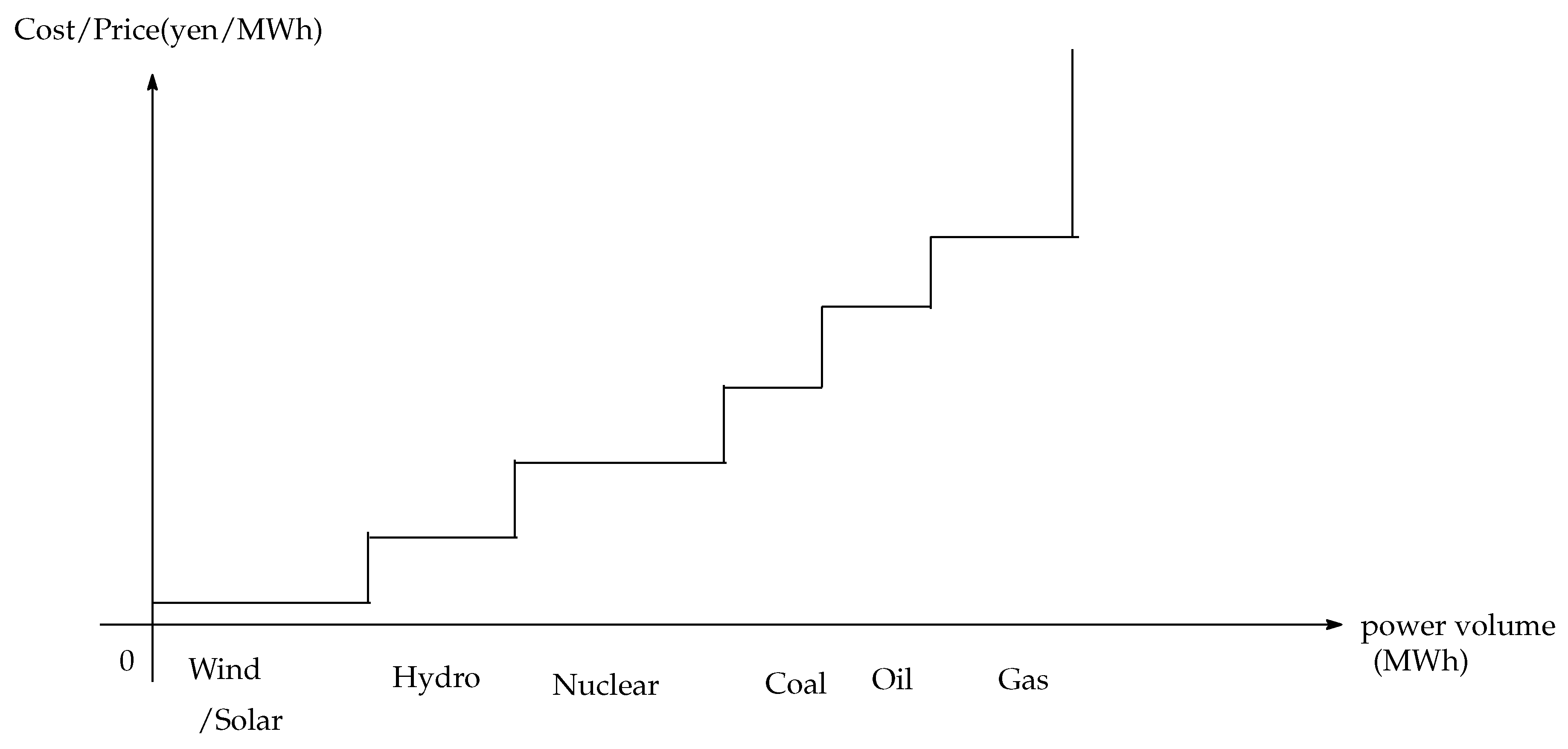
Cost function follows the “merit order curve”.
There are two types of suppliers: normal and renewable suppliers.
There are two markets: forward market and spot market.
Consumers’ demand curve is inelastic to the price.
Only non-renewable suppliers have budgets for speculative trading.
All suppliers and consumers are price-takers.
Since the marginal cost is almost constant under the same power generation method, the power generation company efficiently generates power to meet the limits such that marginal costs remain low in accordance with the demand.
In a power market, “merit order effect” is used as a term to describe the mechanism by which the market price is determined. The electric power supply is determined based on the “merit order”; among these, the sources with the cheapest marginal costs (mostly renewable energy sources such as wind power, solar energy, hydroelectric power, and nuclear power) will be sold more quickly. Renewable energy sources such as photovoltaic solar power, wind power, and hydroelectric power are located at the left end in the merit order curve because they have little marginal costs. Based on this, nuclear power, coal, oil, and natural gas follow in order (see
Figure 1).
For the purposes of this study, we assumed that there are two types of suppliers: normal suppliers and renewable suppliers. Although regional monopolistic companies participate in the electricity market, there are no regional differences in power prices in areas other than Hokkaido, and, as a result of inter-regional competition, a single company cannot wield exclusive market power in JEPX. Recently, new suppliers who deal with renewable energy sources have begun to participate in JEPX, but most of them are small and local companies.
This paper’s major results include determining the relationship between forward price and spot price. Two types of products are currently being traded on JEPX: spot market products and forward market products. Moreover, there are four types of forward products: monthly 24-h products, weekly 24-h products, monthly daytime products, and weekly daytime products. For simplicity, we assume that there are two market types in the model: spot market and forward market.
Power demand also has specific characteristics in economic theories. It is well-known that electricity demand is very inelastic to price. Naturally, a major reason is that electricity is an essential item. Electric power is one of the essential infrastructures of modern society, and it is very difficult to live without electric power in countries where urbanization has advanced. The difficulty of saving electricity is another factor of the inelasticity. If an appropriate storage system is not in place, it is inflexible with respect to price, as it is impossible to buy electricity when its price is low and to consume it when its price is high.
In our model, electricity was supplied through two resources: renewable resources where the marginal costs are zero and non-renewable energy resources, such as thermal power, where the marginal costs can be denoted with a positive real number a.
Our model is based on the particular situation of JEPX. In Japan, JEPX, the only power trading market, was established during the trend of electricity liberalization. JEPX was established through investments from electric power companies and new electric power companies, and started trading from 2005 onwards. Since only members of JEPX can trade in the market, general consumers cannot buy electricity directly. Therefore, we assumed that all market players were price-takers. No one has the market power required for controlling electricity prices.
4. Theoretical Method
4.1. Model Settings
We formulated the following equations as an original model. Suppliers can produce electricity at , and they can trade them at . The trading good for is not electricity; rather, it is the right to sell electricity at . Therefore, at date 1, the suppliers who expect higher prices at date 2 have an incentive to buy them, and those who expect lower prices at date 2 have an incentive to sell them.
There are two types of electricity suppliers: renewable suppliers and normal suppliers.
Renewable suppliers can produce electricity by utilizing renewable resources, and their marginal costs thus tend to be zero. They are small firms and have no budgets for speculation.
Normal suppliers are conventional suppliers. They produce electricity at marginal costs . They have budgets for speculative trading.
At , the electricity supplied at is traded in the market. is price, and is price.
At , all firms can watch and determine the trading volume. All suppliers can sell electricity, but only normal suppliers can buy electricity in the market (renewable suppliers have no budgets for this activity).
All suppliers have beliefs about renewable supply at , . If some firms expect high volumes of renewable supply at , they must also expect low electricity prices at , .
They determine their trading strategy based on their beliefs about .
Profit maximization at
is as follows:
x is the selling volume,
is the purchase volume, and
is the value function for
.
They determine the appropriate date for selling their electricity by comparing the prices and marginal costs. For example, if is higher than their expected forward price and higher than marginal cost a, they sell the electricity.
Renewable suppliers are authorized to sell
units of electricity.
is interpreted as the minimum supply value for renewable energy sources (
can be zero). The main problem of renewable suppliers can be expressed as follows:
x is the selling volume, and is the value function for .
At
, renewable suppliers can sell an additional
units of electricity.
is a random variable, and it is realized at date
.
Because their marginal costs amounts to 0, their strategy is simpler than that of the normal suppliers. If , they usually sell electricity at ; otherwise, they tend to wait until .
The main way to solve the problem can be expressed as follows:
Normal suppliers’ strategy at
can be expressed as follows:
Renewable suppliers’ strategy at
is:
Normal suppliers’ strategy at
can be expressed as follows:
Renewable suppliers’ strategy at
can be expressed as follows:
The consumers’ demand is at . This is the industrial firm’s demand. The consumers’ demand at is . We assumed that little elasticity would exist. That is, , and . We assumed , and .
4.2. Model Equilibrium
The market equilibrium is determined by the intersection between the supply and demand. We can solve this model by conducting backward induction.
The equilibrium at
matches the normal electricity noted in
Section 3.
To explain the equilibrium, we note the total electricity sold at date 1 as
.
The market equilibrium is determined with some price
(see
Figure 2).
Total demand
is expressed as follows:
Total supply
is expressed as follows:
The market equilibrium is determined through the intersection of the demand and supply functions:
The electricity price at
,
is expressed as follows:
depends on the renewable supply and the price at , .
The market equilibrium is determined by the intersection of the demand and supply functions:
The belief of depends on the belief of and .
Let be the distribution of the expected price at at price . For solving the equilibrium, we need the following assumption.
Assumption 1. If, for all,.
Although this is an assumption, we check whether this assumption is satisfied through the market equilibrium.
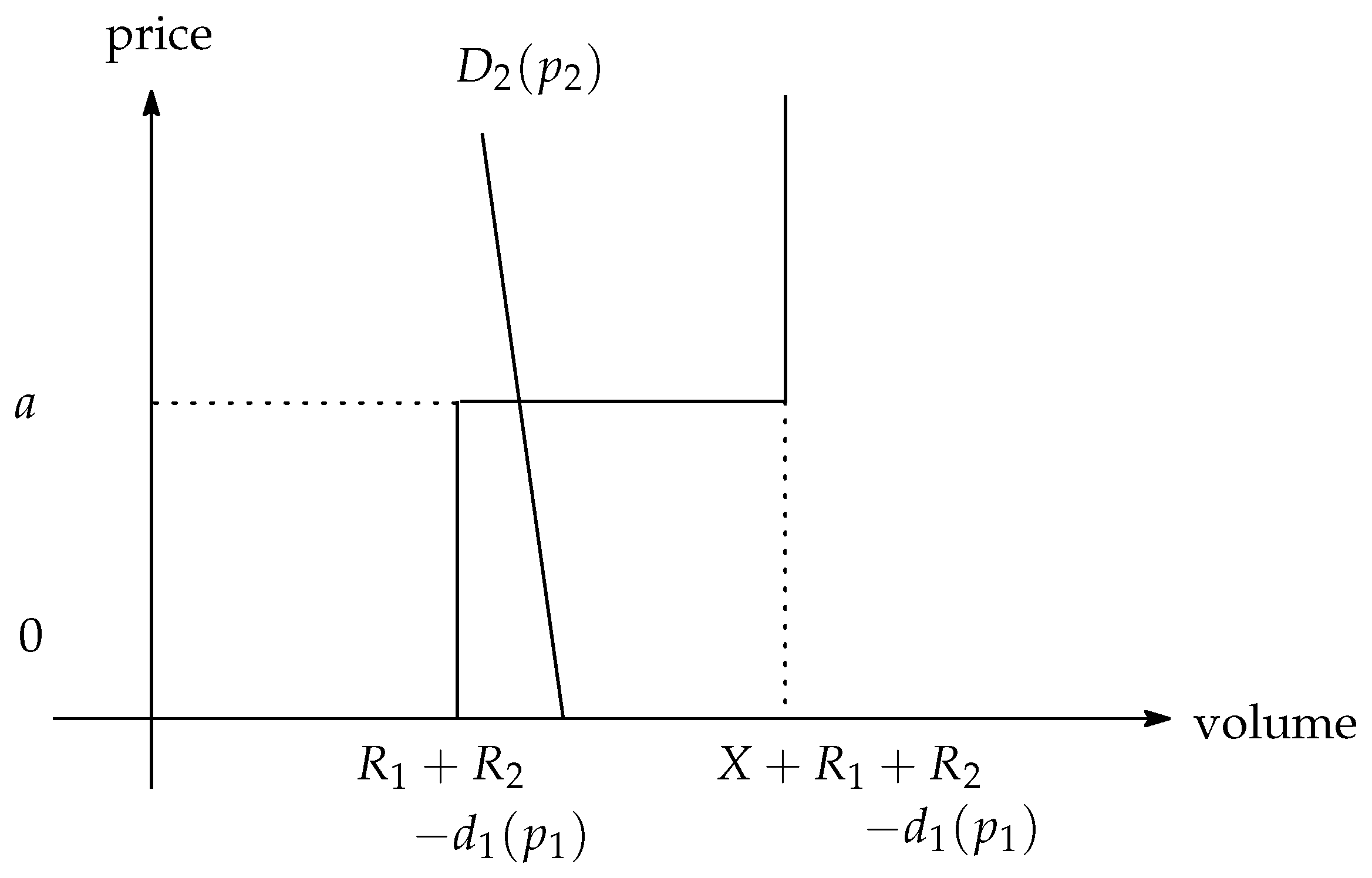
At , the population of suppliers who have beliefs is .
Therefore, at , if , normal suppliers buy electricity, and renewable suppliers sell electricity.
, normal suppliers buy electricity, and renewable and normal suppliers sell electricity.
Total demand
is expressed as follows:
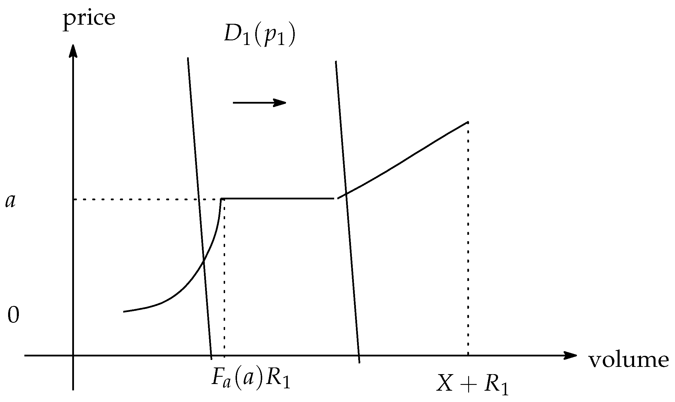
An analysis of Assumption 2 showed that the demand function is decreasing:
, and
. Total supply
is expressed as follows:
An analysis of Assumption 2 showed that the supply function is increasing in
, and
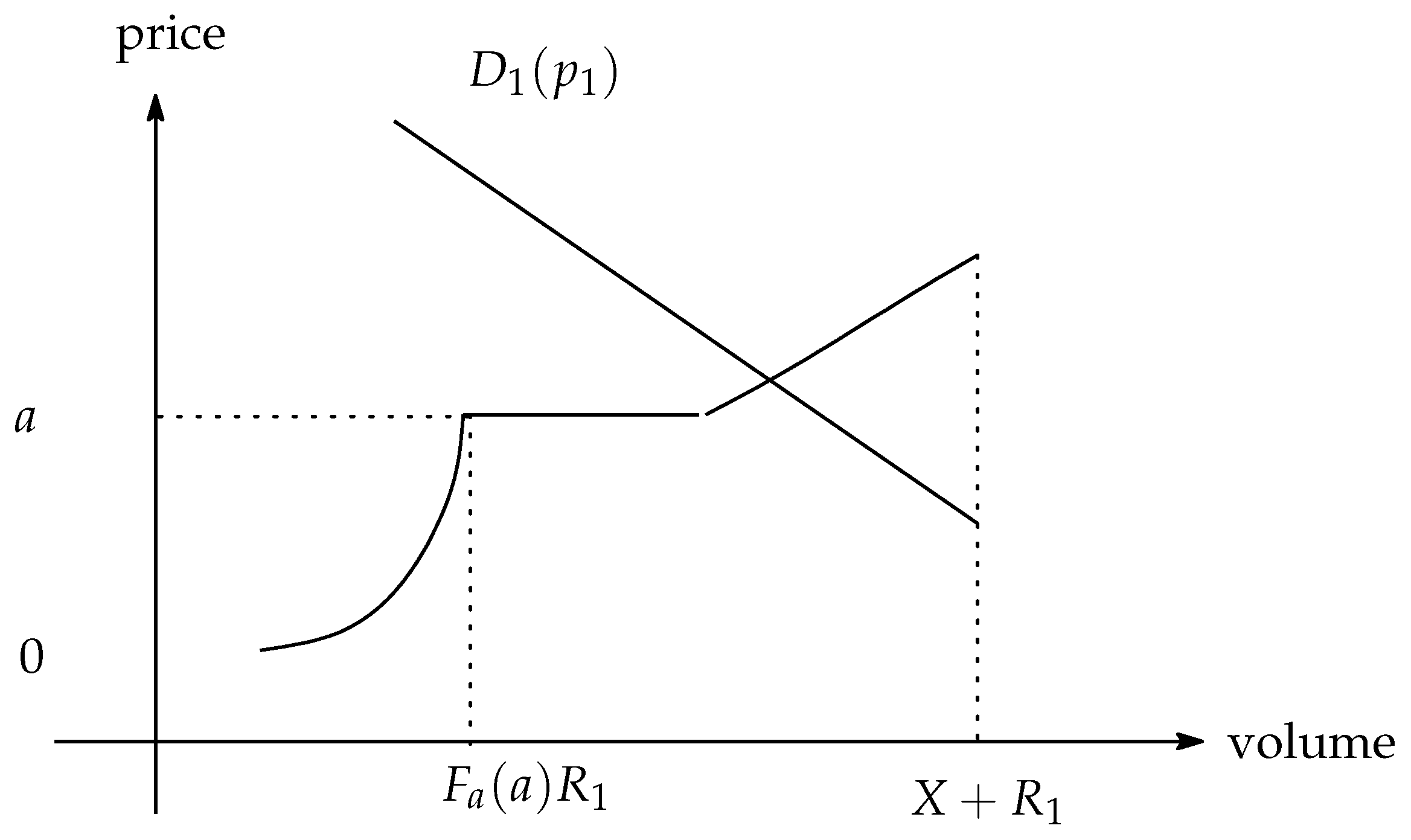
. The market equilibrium is determined by the intersection of the demand and supply functions (see
Figure 3):
The electricity price at
,
is expressed as follows:
is decreasing, and
is increasing.
5. Results and Discussion
This model has a mixed structure; it includes aspects of the heterogeneous belief model as well as the electricity market. Therefore, it includes many special features that are not available in other models. As noted, the shape of supply curve at date 1 is one of them. This shape is derived from the electricity market model. Electricity suppliers have ladder cost-related functions, and their strategy depends on the shape of that functions. We analyzed three major points of this model: price relation, speculative trading effect, and belief effect.
5.1. Price Relation
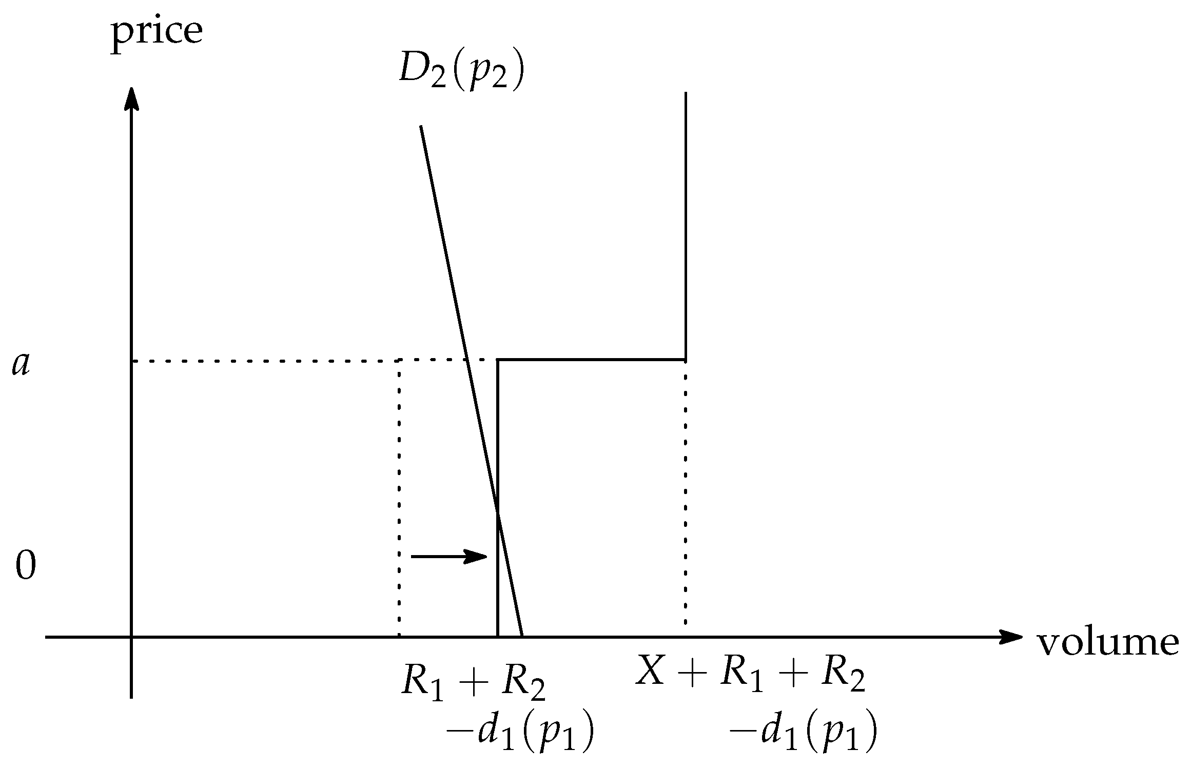
The market at date 2 is simpler than the market at date 1. However, the date 2 price is influenced by the date 1 price . The next lemma shows the relation between and .
The market equilibrium at date 2 is simpler than the date 1 equilibrium. As noted, total supply
is expressed as follows:
electricity units are sold by normal suppliers at date 1. Therefore, based on the date 1 equilibrium, the following can be expressed:
Therefore,
is an increasing function of
. Moreover,
is a decreasing function of
. Thus, if
gets higher (and other conditions at date 2 remain equal), total supply moves towards the right. As a result,
decreases (see
Figure 4).
We can examine Assumption 2 by this price relation. Higher
implies lower
for all suppliers; therefore,
for all
.
This implies that Assumption 2 is satisfied by this equilibrium.
5.2. Speculative Trading
Interestingly, the date 1 supply spikes at price . The optimistic normal suppliers have the incentive to sell electricity at date 1, but their marginal cost is a. Therefore, they choose to sell electricity only if exceeds a.
If the speculative trade is prohibited, the market structure become very simple. Suppliers cannot buy electricity at
; that is,
must be 0. Therefore, normal suppliers’ profit maximization at
changes as follows:
is the selling volume, and
is the value function for
.
The renewable suppliers face the same problem. Thus, the market without speculative trading equilibrium is as follows:
Because suppliers cannot buy the electricity, the demand on date 1 is only .
Because optimistic suppliers expect that renewable supplies are low and electricity prices at is high, they buy date 1 electricity for the purpose of making profits through resale. The date 1 price is affected by the elasticity of the demand. Even if the consumers’ demand is inelastic with regard to the price, total demand is not inelastic with regard to the price.
Lemma 1. The total demand becomes more elastic with regard to the price through speculative trading at.
Proof. In the speculative trading model, the date 1 total demand is elastic.
Even if the consumers’ demand is perfectly inelastic with regard to the price, the total demand is not inelastic with regard to the price. □
This simple lemma implies that the trade of the suppliers has a role in establishing stability in the electricity market. If speculative trade is prohibited, the price
jumps from 0 to
a, with demand for
shifting (see
Figure 5).
Governments may often worry about consumers’ surplus in the speculative electricity market. Interestingly, consumers’ surplus is not always lower than that of the market without resale.
5.3. Heterogeneous Belief
The market equilibrium is heavily influenced by the suppliers’ beliefs. It is essential to compare some measures of optimistic beliefs.
Assumption 2. .
This means that, with distribution , for all , the population that expects to encounter a date 2 price that is higher than , which is larger than that with . Therefore, is a more optimistic distribution than .
Lemma 2. The market priceis higher undercompared to that under.
Proof. This implies
under
is lower than that under
for all
d. Similarly,
is higher than that under
. Then, the date 1 price
p is lower than that under
. This is because the date 2 price
is expressed as follows:
Based on the assumption, for all,
is expressed as follows:
Therefore, the total demand under is larger than that under , and the total supply under is less than that under . As a result, the market price increases under . □
Because of heterogeneous beliefs, the price of the electricity is higher compared to the no-resale market price. Firms have the incentive to buy the electricity for the speculative resale, and the consumer suffers the higher prices.
This model involves a heterogeneous bubble. Heterogeneous beliefs among investors create such bubbles. In such models, investors’ beliefs differ because they have different prior belief distributions. Agents’ heterogenous beliefs can occur because of many factors. For example, overconfidence about the precision of signals among investors can lead to different prior distributions (with lower variance) regarding the signals’ noise term. Investors without common prior beliefs can agree to disagree even after they share all their information with each other. In the heterogeneous beliefs model with short-sale constraints, the asset price can result in the creation of bubbles. Optimistic agents buy the asset, and the price rises. Under the conditions of a short-sale constraint, pessimistic traders cannot make use of the high asset prices (Miller (1977) [
19], Harrison et al. (1978) [
20]). In a dynamic model, the asset price can even exceed the valuation of the most optimistic investor’s expectation regarding the economy. In the model, firms with pessimistic beliefs about the demand on the next day sell the electricity immediately; this implies that the supply on the next day increases. Therefore, a pessimistic belief distribution, such as G(x), is very beneficial for the consumers’ surplus.
As noted in
Section 4.1, higher
implies lower
in this model. Therefore, the next lemma shows some negative correlations between the expected price and the realized price.
Lemma 3. The market priceis lower underthan that under.
Therefore, if the suppliers’ belief is optimistic (that is, they expect higher ), tends to be lower. This can be interpreted as a heterogeneous belief bubble, and this bubble burst on date 2.
6. Policy Implications and Conclusions
6.1. Policy Implications
By utilizing the three lemmas discussed in
Section 5.2 and
Section 5.3, we can propose two policy implications. First, through speculative trading, electricity price spikes can be reduced. Pricing is one of the signals for market conditions. Therefore, in terms of efficiency, price jumping is not desirable. Price spikes are considered in several research papers (Huisman et al. (2003) [
9], Weron et al. (2004) [
26] and others as noted in
Section 2). Price spikes occur because the electricity market is characterized by inelastic demand and a stair-like supply curve. However, speculative trading allows suppliers to be electricity buyers on date 1. This increases the elasticity of the total demand, and the price change becomes relaxed.
Abrupt price fluctuations are undesirable because they increase the market risk. The presence of forward markets is motivated by speculation, so they become more sensitive to price differences. As a result, forward market will be effective for reducing price fluctuations.
Second, the forward market is also an important factor for making policy decisions that may cause prices to move in the opposite direction. If the price on date 1 is large, the price on date 2 tends to be lower. As the government’s main policy target includes consumers who lack market power, it is important to keep the price of the second quarter (that is, the real-time price) low.
The main risk posed by forward markets may be the speculative price hikes. In the case of other asset bubbles, high prices are factors that can hurt efficiency. However, the situation is different in the case of the electricity market. The power market cannot save power because of the characteristics of power; therefore, the power capacity within a certain time zone loses the opportunity cost if it is not sold. Therefore, prices do not remain high, as is the case for ordinary assets. As a result, it is unlikely that the consumer’s utility will be impaired by the high electricity prices. Conversely, as Lemma 2 shows, price increases in the forward market are likely to increase consumer utility. From this viewpoint as well, the effectiveness of the forward market for electricity can be demonstrated.
6.2. Conclusions
Increasing market liquidity is an indispensable factor for introducing renewable energy. However, attempts to raise liquidity in economics can generally lead to speculative behavior. In this paper, we outline such problems with a simple model. Based on the results of the model’s speculative behavior, we determined that, even if the consumer demand for electricity is inelastic with regard to the price, the price elasticity of the demand is newly born; in this way, price change becomes stable. However, the forward market creates speculative trading. Speculative trading naturally accompanies a decrease in consumer surplus. Policymakers, especially the Japanese government, have a strong tendency to vigorously construct speculative actions in the electricity market and strengthen regulations. However, this model shows that some regulation, in terms of optimistic prospects to the future electricity price, can increase consumers’ surplus.
In addition, it has often been pointed out that, in the existing power market model, the market price is dominated by several corporations. In this situation, the market price can be easily raised by these corporations because of the special nature of electric power. However, in this model, the company is assumed to be a price-taker; this also shows that there are cases in which consumer surplus can increase. Thus, inviting new corporations is an important policy for the liberalization of the power market. Our main findings is that the speculative tradings can improve the inelasticity of the demand. This finding of our theory is the first one that points out this effect. This finding is also a very useful result when considering the market design of the electricity market. Speculative trading is an important factor in introducing the forward market to electricity. The results of this paper show that speculative trading has a positive externality and is likely to be a desirable policy in the electricity market.
Our model is based on JEPX. However, the basic elements are common to electricity markets in other countries, and can be applied as a more general electricity model. It would be necessary to comprehensively analyze the linkage between dynamic markets rather than individual markets. We propose a basic model as one of the attempts to describe these two types of markets.


