Article

Short-Term Forecasting of Wake-Induced Fluctuations in Offshore Wind Farms

by
Arslan Salim Dar
1,2,* and
Lüder von Bremen
1,3
1
ForWind-Center for Wind Energy Research, Department of Physics, Carl von Ossietzky University of Oldenburg, 26129 Oldenburg, Germany
2
Wind Engineering and Renewable Energy Laboratory (WIRE), École Polytechnique Fédérale de Lausanne (EPFL), 1015 Lausanne, Switzerland
3
Department of Energy Systems Analysis, DLR-Institute of Networked Energy Systems e.V., 26129 Oldenburg, Germany
*
Author to whom correspondence should be addressed.
Energies 2019, 12(14), 2833; https://doi.org/10.3390/en12142833
Submission received: 21 May 2019 / Revised: 10 July 2019 / Accepted: 17 July 2019 / Published: 23 July 2019
(This article belongs to the Section A3: Wind, Wave and Tidal Energy)

Abstract

:
The increasing share of offshore wind energy traded at the spot market requires short term wind direction forecasts to determine wake losses and increased power fluctuations due to multiple wakes in certain wind directions. The information on potential power fluctuations can be used to issue early warnings to grid operators. The current work focuses on analyzing wind speed and power fluctuation time series for a German offshore wind farm. By associating these fluctuations with wind directions, it is observed that the turbines in double or multiple wake situations yield higher fluctuations in wind speed and power compared to the turbines in free flow. The wind direction forecasts of the European Center for Medium-Range Weather Forecast model are compared with Supervisory Control and Data Acquisition (SCADA) data observations of the turbine yaw. The cumulative probability distribution of the difference in forecasted and observed wind directions shows that for a tolerance of +/−10 , 71% of the observations are correctly forecasted for a lead time of 1 day, which drops to 54% for a lead time of 3 days. The circular continuous rank probability score of the observed wind directions doubles over the lead time of 72 h.

1. Introduction

In modern power systems, high shares of conventional generation (fossil, nuclear) are replaced with fluctuating renewable energies. In the past forecasting tools to predict the generation of PV and wind power plants became essential for safe and economic grid integration. In general, increasing shares of wind and solar generation capacities require higher and regionalized forecast skills of feed-in for power trading, re-dispatch and grid congestion management. Wind power forecasting skills using ensemble prediction methods devised from numerical weather prediction models have been assessed in [1,2]. In particular, large local generation capacities like offshore wind farms ask for specialized short-term (<48 h) forecasts associated with uncertainty information (quantiles) and intra-hour information on power fluctuations. Very strong intra-hour power fluctuations have been observed at various offshore wind farms [3]. The implications to grid integration in the case of the offshore wind farm Horns Rev are outlined in [4]. Lately, research focussed on power fluctuations caused by mesoscale wind fluctuations ([5,6,7]) that occur in specific meteorological conditions (e.g., open cellular convection (OCC)).
In this paper we characterize and investigate observed power fluctuations of an offshore wind farm caused by double and multiple wake situations that do only occur for very distinct wind directions (e.g., along a row of turbines).
The impact of wakes on (mean) power performances and losses of offshore wind farms are studied for a long time (e.g., [8,9]) and smart wind turbine layouts derived with dedicated wake models (e.g., [10] or [11]) try to minimize power losses. Different wake models have been used traditionally to estimate wake losses in planning phase of offshore wind farms (e.g., Fuga [12]). More specifically to wind direction dependencies, Dahlberg [13] found that wake effects have a major impact on power performance along the rows of turbines for the Lillgrund offshore wind farm.
These methods, however, do not account for power fluctuations at time scales that matter for grid integration. Mehrens and von Bremen [14] proposed different methods to characterize mesoscale wind speed fluctuations using data from the offshore met mast FINO1. They concluded that rather simple detection methods can be used to detect situations of fluctuating wind speeds which are relevant for wind power integration. Such a method is adopted to compute wind speed and power fluctuations in this study to detect increased power fluctuations when double and multiple wake situations occur for distinct wind directions.
Double and multiple wake situations on a short time scale get important for two major reasons: (i) grid stability [15] and (ii) predictive control of wind turbines to reduce loads.
The motivation for this paper is to forecast fluctuations with lead times up to 72 h that occur due to double and multiple wake situations in offshore wind farms. The objective is to analyze the occurrence of fluctuations in wind speeds and power by different wake situations and to forecast wind directions that lead to increased fluctuations. Precise forecasts of wind directions are necessary as the wind direction interval for wake situations is generally very narrow.
The paper is organized as follows: the site under consideration and data used in the study is described in Section 2. Section 3 describes the methodology used, including the used method for fluctuation measure, wake detection and processing of the Numerical Weather Prediction (NWP) data. The results from the study are presented in Section 4 and a summary of the work is given in Section 5.

2. Site and Data Description

Wind speed and power fluctuations are characterized for the German offshore wind farm Riffgat, which consists of 30 Siemens SWT-3.6-120 turbines. The hub height is 90 m and the turbine spacing ranges between 4.5 and 5 rotor diameters (Figure 1). The data used is obtained from the Supervisory Control and Data Acquisition (SCADA) systems of all individual turbines. The temporal resolution of data is 5 min and it consists of wind speed, power and yaw angle measurements for the years 2014 and 2015. The data is checked for plausibility in the sense that data entries with no power production due to wind speeds exceeding turbine cut-off are removed from the respective time series. For short-term wind forecast in the years 2014 and 2015, data from the European Center for Medium-Range Weather Forecasts (ECMWF) is used. Wind speed components at the height of 100 m are interpolated to the site of the wind farm Riffgat. Afterwards wind speeds and wind directions are computed. The used lead time of the forecasts is 72 h and the forecasts are initialized twice a day i.e., at 00 and 12 UTC, respectively. The ECMWF model generates forecast data on an hourly basis, whereas, the Riffgat data has a resolution of five minutes. In order to make the two datasets compatible, only information from SCADA data for the same time stamps of the ECMWF forecasts are used to assess wind direction forecast skill.

3. Methodology

3.1. Fluctuation Measure

Based on wind speed and power time series, fluctuation time series were computed using the squared increment sum method described in [14]. It uses a running window over the entire time series and calculates difference between two consecutive measurement values, squares them (for increased sensitivity) and sums over a certain window length. It is ensured that for each time window all time stamps in the original time series are valid, otherwise, no fluctuation is computed for the time window. This method is sensitive to the length of the selected time window selected. Two different time windows (2 h, 6 h) were tested and fluctuation values are normalized with the number of time steps. The following equation is used to compute the fluctuation measure
i n c = 1 n 1 i = 1 n 1 | x i + 1 x i | 2 ,
where x is the quantity of interest, i.e., wind speed or wind power. In consistency with results in [14], it is found that for longer window length, the fluctuation measure becomes smaller. In this paper, the fluctuation measure was computed with a 2 h window and was centered at the time stamp in the middle of each window. Figure 2 shows the wind speed fluctuation measure for window length of two hours at wind turbine R01. In general, the fluctuations were higher in winter and autumn compared to summer and spring. The fluctuation time series were computed for all wind turbines, individually and for the whole wind farm.

3.2. Wake Detection

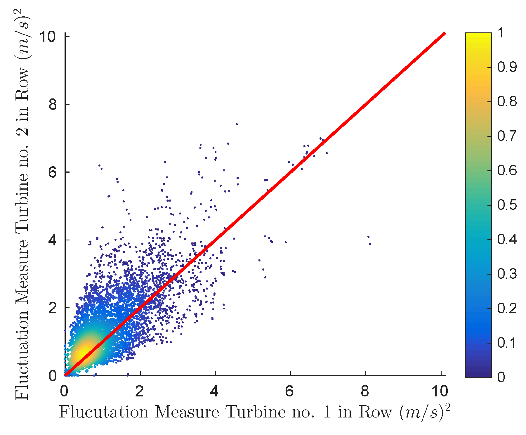
The fluctuation time series computed in the previous section are used to detect wake situations. For this reason, it was necessary to relate computed fluctuations with specific wake situations. This can be done by comparing the observed fluctuations of a free flow turbine with a turbine that is located in the wake at a certain directional sector. If the downstream turbine has higher fluctuations, it can be concluded that it is in the wake of the up stream free flow turbine.
Figure 3 shows the comparison of fluctuations observed at the turbines R01 and R02 for the westerly wind sector (247.5 –262.5 ). The majority of the data lies above the diagonal, which indicates a higher fluctuation at turbine R02 than at R01 for a certain time stamp. This higher fluctuation observed at R02 can be related to the fact that it is in the wake of R01.
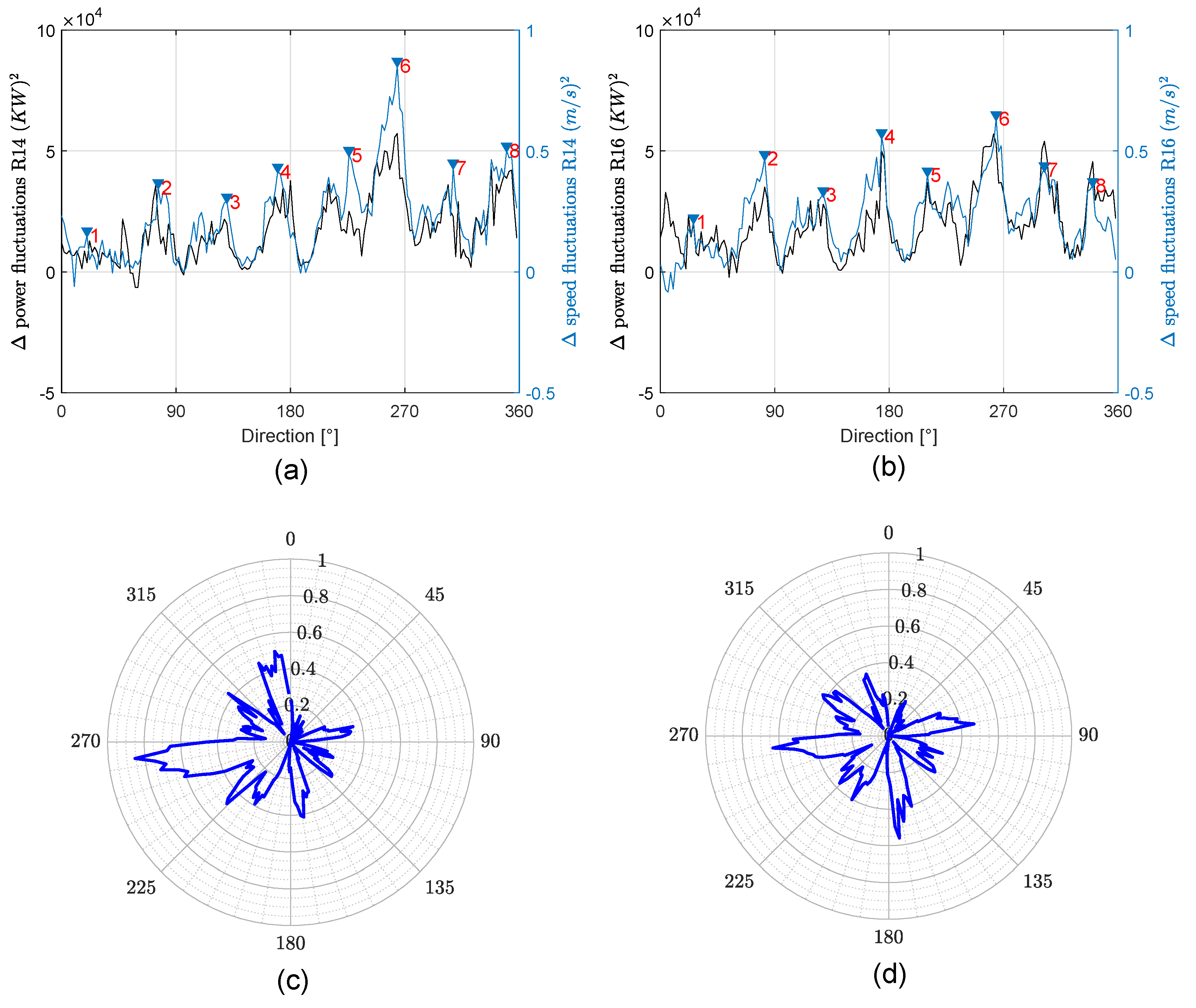
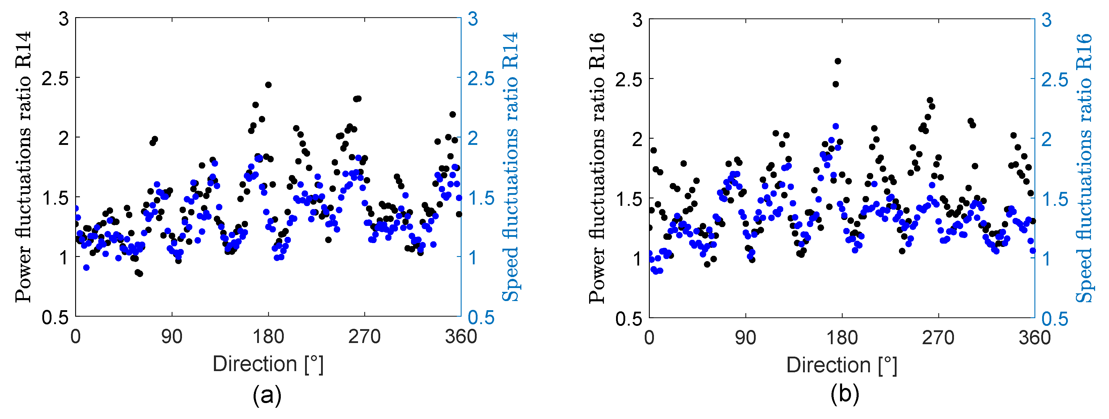
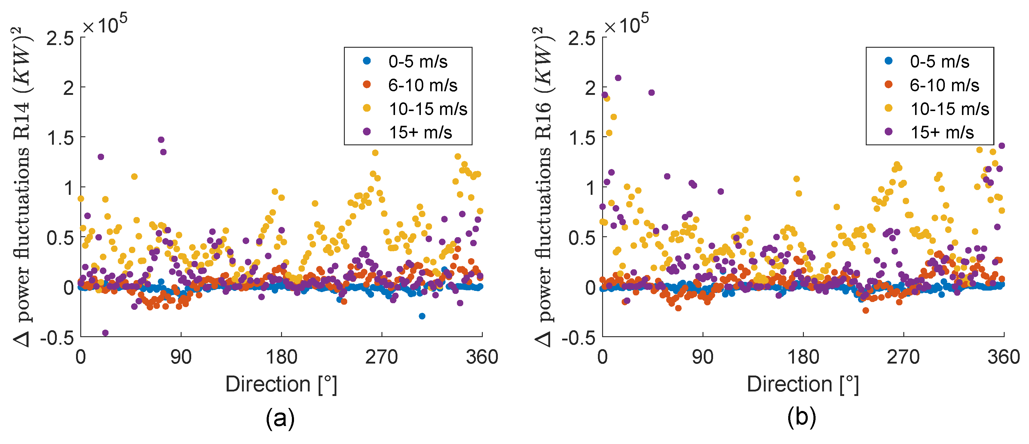
Two measures were used to illustrate fluctuation enhancement. In one case, the difference between fluctuation values of turbine in wake and corresponding turbine in free flow was computed. Alternatively, the ratio between fluctuations of the wake turbine and the free flow turbine was used. Both time series were conditioned to 180 wind direction sectors of 2 width and bin averages are computed.
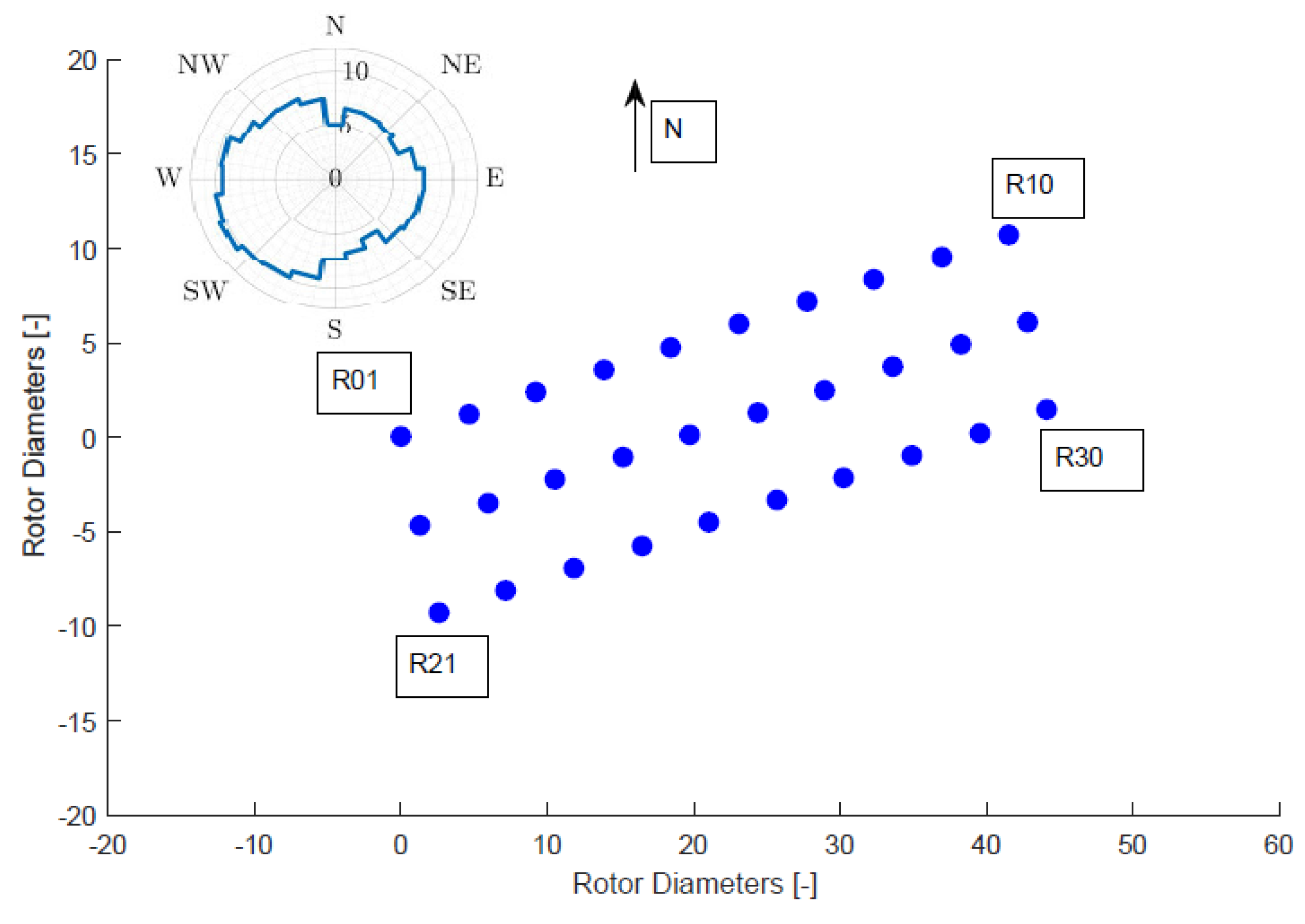
For the turbines fully surrounded by other turbines in all directions (R12–R19) the difference and the ratio of fluctuations with respect to turbines in free flow were computed. Turbines R01, R10, R11, R20, R21 and R30 are taken as free flow turbines in NW, NE, W, E, SW and SE direction respectively. For the north and south directions, however, the closest turbine in free flow in the respective direction is taken as reference. The occurrence of single or multiple wake situations is governed by the wind direction and can be identified by associating wind directions with the geometry of wind farm.

3.3. Wind Direction Forecast Skill

The forecast skill of wind direction forecasts from the ECMWF model for a lead time of 72 h was assessed. The yaw angle of the wind turbine was used as a substitute for the observed wind direction. Figure 4 shows the comparison of turbine yaw angles with wind direction forecast for lead times of 72 h for turbines R01 and R11. However, a negative (or positive) forecast bias can be seen, as the majority of the observations were above (or below) the diagonal. This yaw misalignment is further discussed in the following section and requires correction.
In order to quantify the skill of ECMWF wind direction forecasts, the root mean square error (RMSE) and correlation between the forecast and actual yaw angles and circular correlation is computed. The correlation between the two wind direction datasets requires circular wrapping of data, which was accounted by using the correlation coefficient [16]:
ρ = k = 1 n s i n ( x 1 , k M 1 ) s i n ( x 2 , k M 2 ) k = 1 n s i n 2 ( x 1 , k M 1 ) k = 1 n s i n 2 ( x 2 , k M 2 ) ,
where x 1 , k , x 2 , k are the two sets of directions available and M 1 and M 2 are the averaged directions of the two datasets.
The root mean square error for wind direction data was computed as follows:
R M S E = σ 1 ρ 2 ,
where, σ is the circular standard deviation of directional dataset obtained from yaw angles of turbines.

3.4. Yaw Correction

While analyzing SCADA data for wind directions, varying offset values have been observed for the turbines (Figure 4). It can be concluded that the north of each turbine did not match with real north direction. This mismatch was possibly caused during the construction phase of the wind farm when the nacelle body is placed on top of the tower.
The first step in correction of yaw misalignment was selecting a reference dataset with supposedly correct wind directions. Unfortunately, it was not possible to know if any turbine had the correct directional alignment. The ECMWF data with lead time of 72 h is, therefore, selected as reference data assuming the wind direction forecast of ECMWF has no systematic error (bias). This has been checked with independent FINO1 [17] observations. For the purpose of finding the offset, a linear regression is done. The Y-intercept of this regression yields the value of yaw correction for each individual turbine. Yaw angle observations for all turbines are corrected with the respective offsets found. The average wind direction time series for the whole wind farm was computed using the corrected yaw angles of all individual turbines and was used throughout the study when the whole wind farm is concerned.

4. Results

4.1. Wake-Induced Fluctuations

Figure 5 shows the mean fluctuation difference for speed and power between in-wake turbines (R14, R16) and free flow turbines. Eight different peaks can be identified. The polar plots illustrate the directions causing highest fluctuation differences and the comparison with the geometry of wind farm when wake situations occur. Due to the fine bin width and the phenomena of wake expansion, the maximum peak of a certain direction is observed to be accompanied by several smaller peaks, yielding a width of approximately 30 . It is important to state that directional dependency of wake-induced fluctuations can be identified with a metric that was primarily developed to detect mesoscale wind fluctuations.
Obviously, the peaks of fluctuation enhancement for wind speed and power occur at similar locations. As wind power scales with the cube of wind speed, the quantitative values for wind power fluctuations are on average slightly higher than for wind speed fluctuations. This yields higher fluctuation ratios for power than for wind speed as can be seen in Figure 6 for the wind turbines R14 and R16.
The non-linear wind turbine power curve motivates to analyse whether the strength of wake-induced power fluctuations is dependent on the average wind speed. For this purpose, power fluctuation differences are conditioned to mean wind speed of the respective free-flow turbines and to wind direction. The mean wind speed is computed as a 2 h average. Figure 7 shows that highest fluctuations occur in the wind speed interval of 10–15 m/s, where wind speed is fluctuating around the rated wind speed of 12–13 m/s. Conclusively, sometimes the nominal power is reached and sometimes not, while the free-flow turbine is steadily operating at the nominal power. In addition, the wake-induced and free flow fluctuations are smaller when wind speeds are consistently above the rated wind speed i.e., >15 m/s. For lower wind speed intervals, the fluctuations are relatively insignificant at all wind directions.
While the study of fluctuations for individual turbines is interesting for load management and control of wind turbines, power fluctuations of the whole wind farm are important from the grid integration perspective. The fluctuations of the whole wind farm are expressed relative to the fluctuations of a single reference free-flow turbine. The power fluctuation time series of the whole wind farm is computed from the average wind power time series of the whole wind farm. Depending on the wind direction the power fluctuation time series of a free-flow wind turbine in one of the corners of the wind farm is used as reference power fluctuation time series.
A rose plot of the ratio of fluctuation of the whole wind farm to the fluctuation of the reference free-flow turbine is shown in Figure 8. Wind directions with enhanced fluctuations for the whole wind farm can be clearly identified. The smoothing of the wind power time series due to averaging over the whole wind farm results in a ratio consistently lower than 1 for all wind directions.

4.2. ECMWF Wind Direction Forecast Skill

ECMWF wind direction forecasts are validated with the mean SCADA yaw angles which is computed as the average over all the turbines and will be called observed wind direction hereafter. The forecast skill for a specific wind direction sector is important in the proposed applications as the wake-induced fluctuations develop only in specific wind direction intervals. To assess the ability of the ECMWF model to forecast wind directions within certain ranges (sectors), we compute the difference between the corresponding forecasted and observed wind directions (fc-obs). Based on the computed difference, we draw the probability distribution and cumulative probability distribution for lead times of 1 day (0–24 h) and three days (49–72 h) in Figure 9. From the cumulative probability distribution, we can estimate the quality of wind direction forecasts for any particular tolerance in the difference between the two datasets. For instance, if we allow for a range of +/−10 , it can be seen from the cumulative probability that in 29% of the cases a particular wind direction interval was not forecasted (1 day lead time). At day 3, whereas, 46% of the forecasts fall outside the observed wind directions allowing for a tolerance of +/−10 (illustrated with red dotted lines in Figure 9). However, this result means that in 71% of the cases a particular wind direction interval was forecasted correctly (54% for day 3). Note that we discuss the results for a tolerance of +/−10 as Figure 8 suggests that induced fluctuations occur for direction intervals of 20 width or even broader. The broader the tolerance, the better the anticipated forecast skill. In the future, wind directions can be forecasted with ensemble prediction systems providing a distribution of the forecasted wind direction.
In order to simulate this, we put Gaussian distributions with standard deviation of 10 , 15 and 20 around the deterministic forecast and compute the respective circular continuous ranked probability score (CRPS) as a function of lead time (Figure 10). The circular CRPS [18] is a common skill score to assess the quality of a probabilistic forecast and considers the resolution and the reliability of the forecast. The chosen standard deviations are supposed to be representative for a certain sector width. The CRPS almost doubles over the 72 h lead time. It must be noted that in reality the distribution of ensemble members will not be Gaussian. However, it can be seen that the CRPS is not very sensitive to the increased standard deviation. It can be concluded that the CRPS is mainly driven by the deterministic forecast error.
This is supported by the comparison between ECMWF wind direction forecast and observed yaw angles averaged over all wind turbines (Figure 11). The root mean square error roughly doubles for 72 h forecast compared to the zero forecast step. Note, that the random model error of the wind direction is already at the model start considerably high.

5. Conclusions

With the continuous growth of wind energy, the information on potential fluctuations in power on time scales relevant to grid integration becomes essential. In the current work, we characterized wind speed and power fluctuations caused due to wake situations over a time scale of two hours. For this purpose, an increment sum method is used to compute a fluctuation measure for wind speed and power of a German offshore wind farm using a time window of two hours. The computed fluctuation measure is utilized to detect wake situations by comparing the fluctuations between the in-wake turbines and the free flow turbines for certain wind directions. The strongest enhancement in power fluctuations is observed to occur for wind speeds between 10 and 15 m/s. As wind turbine wakes only develop in specific wind directions, the capability of wind direction forecasts from ECMWF over a lead time of 72 h is assessed. The probability distributions of difference between the forecasts and observed wind directions for lead times of one and three days are computed. These probability distributions show that for a tolerance of +/−10 , 71% of the forecasts correctly predict the observed wind directions for lead time of one day, whereas, 54% of the forecasts correctly predict the observed wind directions for lead time of three days. In the future, ensembles of wind direction forecasts can be used to alert if certain wind directions will occur.

Author Contributions

This study was done as a part of A.S.D.’s internship at ForWind, supervised by L.v.B.

Funding

This research received no external funding.

Conflicts of Interest

The authors declare no conflict of interest.

References

  1. Pinson, P.; Nielsen, H.A.; Madsen, H.; Kariniotakis, G. Skill forecasting from ensemble predictions of wind power. Appl. Energy 2009, 86, 1326–1334. [Google Scholar] [CrossRef] [Green Version]
  2. Alessandrini, S.; Sperati, S.; Pinson, P. A comparison between the ECMWF and COSMO Ensemble Prediction Systems applied to short-term wind power forecasting on real data. Appl. Energy 2013, 107, 271–280. [Google Scholar] [CrossRef]
  3. Akhamatov, A.; Rasmussen, C.; Eriksen, P.B.; Pedersen, J. Technical aspects of status and expected future trends for wind power in Denmark. Wind Energy 2007, 10, 31–49. [Google Scholar] [CrossRef]
  4. Sorensen, P.; Cutululis, N.A.; Vigueras-Rodriguez, A.; Jensen, L.E.; Hjerrild, J.; Donovan, M.H.; Madsen, H. Power fluctuations from large wind farms. IEEE Trans. Power Syst. 2007, 22, 958–965. [Google Scholar] [CrossRef]
  5. Vincent, C.; Pinson, P.; Giebel, G. Wind fluctuations over the North Sea. Int. J. Climatol. 2010, 31, 1584–1595. [Google Scholar] [CrossRef]
  6. Vincent, C.L.; Hahmann, A.N.; Kelly, M.C. Idealized mesoscale model simulations of open cellular convection over the sea. Bound.-Layer Meteorol. 2012, 142, 103–121. [Google Scholar] [CrossRef]
  7. Mehrens, A.R.; von Bremen, L.; Larsen, X.; Hahmann, A. Correlation of mesoscale wind speeds in the North Sea. Q. J. R. Meteorol. Soc. 2016, 142, 3186–3194. [Google Scholar] [CrossRef]
  8. Frandsen, S.; Barthelmie, R.; Pryor, S.; Rathmann, O.; Larsen, S.; Hojstrup, J.; Thogersen, M. Analytical modelling of wind speed deficit in large offshore wind farms. Wind Energy Int. J. Prog. Appl. Wind Power Convers. Technol. 2006, 9, 39–53. [Google Scholar] [CrossRef]
  9. Japar, F.; Mathew, S.; Narayanaswamy, B.; Lim, C.M.; Hazra, J. Estimating the wake losses in large wind farms: A machine learning approach. In Proceedings of the ISGT, Washington, DC, USA, 19–22 February 2014; pp. 1–5. [Google Scholar]
  10. Schmidt, J.; Stoevesandt, B. The impact of wake models on wind farm layout optimization. J. Phys. Conf. Ser. 2015, 625, 012040. [Google Scholar] [CrossRef]
  11. Kirchner-Bossi, N.; Porté-Agel, F. Realistic Wind Farm Layout Optimization through Genetic Algorithms Using a Gaussian Wake Model. Energies 2018, 11, 3268. [Google Scholar] [CrossRef]
  12. Ott, S.; Nielsen, M. Developments of the Offshore wind Turbine Wake Model Fuga; No. 0046; DTU Wind Energy: Roskilde, Denmark, 2014. [Google Scholar]
  13. Dahlberg, J.A. Assessment of the Lillgrund Wind Farm: Power Performance Wake Effects; 61 LG Pilot Report; Vattenfall Vindkraft AB: Solna, Sweden, 2009. [Google Scholar]
  14. Mehrens, A.R.; von Bremen, L. Comparison of methods for the identification of mesoscale wind speed fluctuations. Meteorol. Z. 2017, 26, 333–342. [Google Scholar] [CrossRef]
  15. Tande, J.O.G. Grid integration of wind farms. Wind Energy 2003, 6, 281–295. [Google Scholar] [CrossRef]
  16. Fisher, N.I.; Lee, A.J. A correlation coefficient for circular data. Biometrika 1983, 70, 327–332. [Google Scholar] [CrossRef]
  17. FINO1 Data Courtesy. Available online: http://www.bsh.de/de/Meeresdaten/Projekte/FINO/index.jsp (accessed on 27 March 2017).
  18. Grimit, E.P.; Gneiting, T.; Berrocal, V.J.; Johnson, N.A. The continuous ranked probability score for circular variables and its application to mesoscale forecast ensemble verification. Q. J. R. Meteorol. Soc. J. Atmos. Sci. Appl. Meteorol. Phys. Oceanogr. 2006, 132, 2925–2942. [Google Scholar] [Green Version]
Figure 1. Layout of the Riffgat wind farm. The wind rose is computed from Supervisory Control and Data Acquisition (SCADA) data of the years 2014 and 2015.
Energies 12 02833 g001
Figure 2. Wind speed fluctuation time series at wind turbine R01 for a time window length of two hours.
Energies 12 02833 g002
Figure 3. Density plot of wind flucutations at wind turbine R02 versus free-flow wind turbine R01 for the westerly wind sector.
Energies 12 02833 g003
Figure 4. Density plots between forecast wind direction and observed yaw angles for (a) wind turbine R01 and (b) wind turbine R11 for lead time 72 h.
Energies 12 02833 g004
Figure 5. Mean fluctuation difference (a,b) between inner turbines and free-flow turbines for all wind directions and wind turbines R14 (c) and R16 (d), respectively. Left axis shows power fluctuations and right axis shows wind speed fluctuations. Polar plot of wind speed fluctuation difference for turbines R14 and R16, respectively. The radial axis is the difference of wind speed fluctuations [(m/s) 2 ] between inner turbine and a free-flow turbine.
Energies 12 02833 g005
Figure 6. Ratio of fluctuations between in-wake and free-flow wind turbines for (a) R14 and (b) R16.
Energies 12 02833 g006
Figure 7. Difference of fluctuations characterized with respect to wind speed intervals for (a) R14 wind turbine and (b) R16 wind turbine.
Energies 12 02833 g007
Figure 8. Wind power fluctuation enhancement of the whole wind farm for certain wind directions. The radial axis is the ratio of fluctuations between the whole wind farm and a free-flow reference wind turbine.
Energies 12 02833 g008
Figure 9. (Top) Probability distribution and (bottom) cumulative probability distribution of the difference between the forecasted and observed wind directions. Black line represents lead time of one day (0–24 h) and green line represents lead time of three days (49–72 h).
Energies 12 02833 g009
Figure 10. Circular continuous rank probability score for the observed wind directions for lead times from 0–72 h. Black solid line: standard deviation 10 ; blue dashed line: standard deviation 15 and green dashed line: standard deviation 20 .
Energies 12 02833 g010
Figure 11. European Center for Medium-Range Weather Forecasts (ECMWF) wind direction forecasts skill validated with averaged yaw observations of all wind turbines in terms of root mean square error.
Energies 12 02833 g011

