Article

Unsteady RANS Simulations of Flow around a Twin-Box Bridge Girder Cross Section

Department of Mechanical and Structural Engineering and Materials Science, University of Stavanger, Postboks 8600 Forus, 4036 Stavanger, Norway
*
Author to whom correspondence should be addressed.
Energies 2019, 12(14), 2670; https://doi.org/10.3390/en12142670
Submission received: 21 May 2019 / Revised: 4 July 2019 / Accepted: 8 July 2019 / Published: 11 July 2019
(This article belongs to the Special Issue Engineering Fluid Dynamics 2019-2020)

Abstract

:
The aerodynamic performance of bridge deck girders requires a thorough assessment and optimization in the design of long-span bridges. The present paper describes a numerical investigation of the aerodynamic characteristics of a twin-box bridge girder cross section in the range of angles of attack between −10.0° and +10.2°. The simulations are performed by solving 2D unsteady Reynolds-averaged Navier–Stokes (URANS) equations together with the k–ω shear stress transport (SST) turbulence model. The investigated Reynolds number (Re) based on the free stream velocity ( U ) and the height of the deck (D) is 31,000. The predicted aerodynamic characteristics such as the mean drag, lift and moment coefficients, are generally in good agreement with the results from the wind tunnel tests. Changes of flow patterns and aerodynamic forces with different angles of attack are investigated. Flow characteristics during one vortex shedding period are highlighted. Relative contributions of each of the two bridge decks to the overall drag and lift coefficients, with respect to the angle of attack, are also discussed.

Graphical Abstract

1. Introduction

In wind-resistant bridge design, many factors should be considered, such as static wind load, wind forces due to turbulence, aerodynamic instability and vortex-shedding excitation. For bridge spans around 1 km and longer, twin-box girders are being increasingly used, due to their favorable aerodynamic properties in term of flutter stability. This is due to a favorable effect of the central gap on the surface pressure distribution, and a higher ratio between the twisting and the heaving eigen-frequencies [1,2]. On the other hand, this configuration is prone to vortex-induced vibration, since vortices shed from the windward box can cause a significant excitation of the leeward box and thereby important oscillations of the bridge girder [3,4]. In the early design stage of long-span bridges, several bridge deck design alternatives are usually considered, and their aerodynamic performance must be assessed to ensure the most feasible design for the specific project.
Both experimental and numerical approaches are available for the assessment of the bridge deck aerodynamic performance [4,5]. Extensive wind tunnel experiments are normally performed to optimize the design of long-span bridges. However, wind tunnel investigations have limitations in terms of time, cost, applicable Reynolds numbers and the representation of the details such as railings and stabilizers at small scales. For an improved bridge design, computational fluid dynamics (CFD) based simulations can facilitate a deeper understanding of complex flow conditions around a bridge girder, as demonstrated by [6,7,8,9,10,11,12,13].
The application of a 2D unsteady Reynolds-averaged Navier–Stokes (URANS) model for flow around simple rectangular geometry has been validated thoroughly in previous research [14,15,16,17,18]. Mannini et al. [16] applied 2D URANS equations with advanced turbulence modeling closures for predicting flow around a 5:1 rectangular cylinder at Re = 1 × 10⁵. They found that the predicted force coefficients are in reasonable agreement with the experimental data reported by Schewe [19,20]. Ong [17] conducted CFD simulation for the same structure at high Re numbers (5 × 10⁵, 1 × 10⁶, 1.5 × 10⁶ and 2 × 10⁶) using the 2D URANS together with the standard high Reynolds number k–ω model. For engineering design purposes, it gave reasonably good agreements with the published experimental data in terms of time-averaged drag coefficients, Strouhal numbers and time-averaged base pressure coefficient. Patruno et al. [18] studied the flow field around the 5:1 rectangular cylinder with an angle of attack of 0 to 4 degrees using both Large Eddy Simulation (LES) and URANS (i.e., k–ω shear stress transport (SST)) turbulence models. They found that LES and URANS approaches appeared to provide comparable results in terms of accuracy of first and second order pressure statistics measured at the central section of the considered prism. The asymmetric characteristics of the flow field induced by small angles of attack were under-estimated by LES as compared to URANS simulations, and the experimental data were between them generally.
The main goal of the present study is to evaluate the validity of 2D URANS simulations with k–ω SST turbulence model [21] for the flow around a twin-box bridge girder cross-section. One of the preliminary bare deck designs of the Halsafjord suspension bridge in Norway will be considered in the present study, see Figure 1. This bare deck design was chosen due to the availability of experimental data for validation studies. Several CFD studies of flow characteristics around the sharp-edged twin-boxes, particularly with asymmetric geometry as in the present case, have been carried out [22,23,24]. These studies have mainly dealt with the overall flow conditions and their variations with the relative gap size, Reynolds number and turbulence models used in the simulations. To the authors’ knowledge, there is a limited number of studies addressing the flow characteristics around the bridge girder subject to flow at different angles of attack. The present study will provide a thorough 2D CFD investigation of the flow conditions around the twin-deck inclined to the approaching flow at angles of attack (AoA) ranging from −10.0 to +10.2 degrees (°).
The study utilizes data from a wind tunnel investigation for validation. The tests were performed with a 1:40 section model at Re = 31,000, as reported in [25]. The cross-section geometry and the Reynolds number in the simulations are thus adopted as for the section model, which was exposed to a uniform flow. The results are discussed in terms of the time-averaged drag coefficient ( C D ¯ ), the time-averaged lift coefficient ( C L ¯ ) and the time-averaged moment coefficient ( C M ¯ ) in the range of AoA from −10.0° to +10.2°, respectively. The time histories of the force coefficients as well as the flow physics changes with different AoA are investigated. The vortex shedding process and the associated variation of the instantaneous drag and lift coefficients for each of the two decks with different AoA are also presented and discussed in detail.

2. Mathematical Formulation

2.1. Flow Model

The Reynolds-averaged equations for conservation of mass and momentum are given by:
u j x j = 0
u i t + u j u i x j = 1 ρ p x i + v 2 u i x j x j u i ' u j ' ¯   x j
where i, j = 1, 2. Here x 1 and x 2  denote the streamwise and cross-stream directions respectively; u 1 and u 2 are the corresponding mean velocity components; u i ' u j ' ¯ is the Reynolds stress component, where u i ' denotes the fluctuating part of the velocity; p is the pressure; ρ is the density of the fluid and t is the time.
The k– ω SST turbulence model [26] used in the present study is a blending of the k– ω and the k– ε models. The original k– ω model of [27] is implemented in the near-wall region and the standard k– ε model of [28] in the outer wake region and in the free shear layers. Following [26], the equations for the k– ω SST turbulence model is taken as:
D ( ρ k ) D t = P k ˜ β * ρ ω k + x j [ ( μ + σ k μ t ) k x j ) ]
D ( ρ ω ) D t = α ρ S 2 β ρ ω 2 + x j [ ( μ + σ ω μ t ) ω x j ) ] + 2 ( 1 F 1 ) ρ σ ω 2   1 ω   k x j ω x j
where P k ˜ is given by:
P k ˜ = min [ μ t u i x j ( u i x j + u j x i ) ,   10 β * ρ k ω ]
Here ϕ 1 represents any constant in the original k ω turbulence model (i.e., σ k 1 , β 1 , σ ω 1 ) and ϕ 2 represents any constant in the original k ε turbulence model (i.e., σ k 2 , β 2 , σ ω 2 ) . ϕ , the corresponding constant of the new k ω SST turbulence model given by Equations (3) and (4), is
ϕ = F 1 ϕ 1 + ( 1 F 1 ) ϕ 2
F 1 = tan h ( arg 1 4 )
arg 1 = m i n [ max ( k 0.09 ω y , 500 ν y 2 ω ) , 4 ρ σ ω 2 k C D k ω y 2 ]
C D k ω = m a x ( 2 ρ σ ω 2 1 ω k x j ω x j , 10 10 )
Here y is the distance to the nearest wall and C D k ω is the positive portion of the cross-diffusion term of Equation (4).
The turbulence viscosity can be estimated by:
ν t = a 1 k max ( a 1 ω , S F 2 )        
where S is the invariant measure of the strain rate and F 2 is given by:
F 2 = tan h ( arg 2 2 ) ,   arg 2 = max ( 2 k 0.09 ω y , 500 ν y 2 ω )  
The empirical constants of the k ω SST model are [19]:
β * = 0.09 ,   a 1 = 0.31 ,   α 1 = 0.5532 ,   α 2 = 0.4403 ,   β 1 = 0.075 ,   β 2 = 0.0828 , σ k 1 = 0.85034 , σ k 2 = 1.0 and σ ω 1 = 0.5 ,   σ ω 2 = 0.856 16.

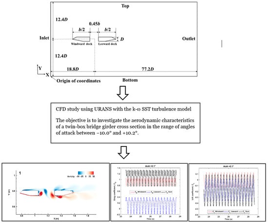
2.2. Numerical Simulation Scheme, Computational Domain and Boundary Conditions

The open source CFD code OpenFOAM [29] is used in the present study. The pressure implicit with splitting of operators (PISO) scheme is chosen for the solver. The spatial schemes for gradient, Laplacian and divergence are Gauss linear, Gauss linear corrected and Gauss linear schemes, respectively. All these schemes are in second order accuracy. The second order Crank–Nicolson scheme is used for the time integration.
Figure 2 shows the investigated twin-box bridge girder cross section and the corresponding computational domain. The size of the entire computational domain is 6 m by 1.55 m, which is equivalent to 91.0D by 24.8D, where D is the height of the girder cross section. The origin of the coordinate system is located at the left lower corner of the domain. The flow inlet boundary is 18.8D upstream from the center of the gap between the decks and the flow outlet boundary is 77.2D downstream from the center of the gap. The top and bottom boundaries are positioned at a distance of 12.4D from the center of the gap between the decks. Although the shear center of the bridge deck section does not coincide with the mid height of the deck, the rotation center is adopted in the middle of the deck height. This facilitates a direct comparison with the experimental results which also refer to such a rotational center. The deck position and the domain size in the Y direction are same as in the wind tunnel working section. The boundary conditions used for the present numerical simulations are as follows:
  • A uniform flow, u 1 = U , u 2 = 0 , is set at the inlet boundary; the pressure is specified as zero normal gradient at the inlet boundary. k and ω at the inlet boundary are set equal to:
    k i n l e t = 0.5 ( U I u + U I v + U I w ) 2
    where I u and I v are the turbulence intensities in X and Y directions, respectively. I u = 12 % and I v = 8 % are taken from [25].
    ω i n l e t = k i n l e t 0.5 / ( C μ 0.25 l )  
    where C μ = 0.09 is the empirical constant specified in the turbulent model and turbulence length l = 0.07D [30,31,32]. Effects of l on the calculated results have been studied by using a much lower value   l = 0.04D, and small variations (less than 0.27%) are observed in the aerodynamic quantities, i.e., mean drag coefficient, root mean square (r.m.s.) of the lift coefficient and Strouhal number.
  • Along the outlet boundary, u 1 ,   u 2 , k and ω are specified as zero normal gradient. The pressure is specified as zero. The zero pressure outlet boundary condition has been widely used to calculate the unsteady flow around bluff bodies [33,34,35]. The distance used in the present study for the downstream 77.2D is considerably longer than the value of 50D previously used by [10]. It is considered that the effect of the outlet boundary condition on the numerical results is negligible.
  • On the deck surfaces, no-slip boundary condition is specified (i.e., u 1 = u 2 = 0 ). The pressure is set as zero normal gradient. k is fixed at 0 and ω is calculated as follows [26]:
    ω d e c k = 10 × 6 ν β 1 ( Δ y 1 ) 2  
  • For the top and bottom boundaries, u 1 = u 2 = 0 , the pressure is set as zero normal gradient; k is fixed at 0. ω is specified as zero normal gradient.

2.3. Grid and Time Resolution Tests

Convergence studies considering different grid sizes and the time steps have been carried out for AoA ranging from −10.0° to +10.2°. Time-averaged drag coefficient ( C D ¯ ), time-averaged lift coefficient ( C L ¯ ), time-averaged moment coefficient ( C M ¯ ) as well as Strouhal number (St) are considered in the tests. The time-averaged values are obtained with a duration of 30 vortex shedding cycles after the numerical results have repeated their cycles. Here the drag coefficient ( C D ), lift coefficient ( C L ), moment coefficient ( C M ) and Strouhal number (St) are defined as follows:
C D = F d r a g 1 2 ρ U 2 D
C L = F l i f t 1 2 ρ U 2 b
C M = M 1 2 ρ U 2 b 2  
S t = f D U  
where F d r a g , F l i f t are the along-wind and the cross-wind force components acting on the decks per unit length and b is the width of the two decks, i.e., of the solid part of the cross-section. M is the overturning moment about the aforementioned rotational center per unit length, and is positive in the clockwise direction. The frequency of vortex shedding f is obtained from CL. Figure 3 shows the sign convention. Like the overturning moment, AoA is defined positive in the clock-wise (nose-up) direction in the cases of wind coming from left to right.
The results of both the grid size and the time step convergence studies in terms of the force coefficients are shown in Table 1 and Table 2, where Δ t . represents the time step in seconds. The relative change of results between two consecutive meshes or time steps is investigated in terms of   C D ¯ , C L ¯ , C M ¯ as well as St. The cases with the converged solution in terms of grid size and time-step are marked with ‘*’ and, adopted for the further investigations.
For most of the cases, the grid resolution tests have been carried out with 3 sets of meshes with 138,354 (M1), 198,834 (M2) and 288,804 (M3) elements and two different time-steps (i.e., M3 with time-step of 5.00 × 10⁻⁵ s, and M3T1 with time-step of 2.50 × 10⁻⁵ s), see Table 1 and Table 2. For example, in the AoA = +0.1° case, the relative change of the C D ¯ values between M1 and M2 meshes is 14.0%. The difference decreases to 1.7% when the mesh is further refined from M2 to M3, i.e., a negligible change is observed. A similar trend is observed for the other cases. For the cases of AoA = +4.4°, +6.3° and +10.2°, 138,354 to 545,954 (or 362,514) elements were used for the grid resolution tests. The convergence is considered to be achieved when the relative variation of the aerodynamic quantities between two cases is lower than 5% or if the parameters change by less than 0.01 in magnitude. For instance, in the AoA = +0.1° case, the relative change of C M ¯ values between M3 and M3T1 cases is 8.2%, the absolute change of the C M ¯ values is less than 0.01, see Table 1. An example of the mesh structure with 288,804 elements, in the case of AoA = +0.1°, is presented in Figure 4.
For the AoA = +0.1° case, the values of y + over the entire wall boundaries of two decks range from 0 to 7.8 with an average value from 1.0 to 1.5, where y + = u * Δ y 1 / ν = τ w / ρ · Δ y 1 / ν , where u * and τ w denote the wall friction velocity and wall shear stress, respectively. The maximum y + value is found at the windward deck at the leading edge lower corner, where high flow acceleration exists. A similar procedure is taken to calculate the averaged y + ¯ for other AoA cases, and the averaged values of y + ¯   give a range of 1.0 to 2.1. All refinement studies of the flow at different AoA are carried out with the fixed y + values in order to minimize influence of the boundary layer calculation.
Overall, it is concluded that the present simulations marked with ‘*’ in Table 1 and Table 2 can provide satisfactory spatial and time resolutions for all the different AoA cases at Re = 31,000.

3. Results and Discussion

3.1. Validation of Numerical Model

To assess the validity of URANS with the k ω SST turbulence model for flow around twin-box girder bridge cross section, a comparison has been carried out between the present simulations and the wind tunnel test results from [18]. The time-averaged aerodynamic quantities such as C D ¯ , C L ¯ and C M ¯ , in the range of AoA from −10.0° to +10.2° at Re = 31,000 are studied, see Figure 5. A good overall agreement between the present numerical simulations results and the experimental data is observed. Generally, the presently predicted C D ¯ are in good agreement with the experimental data for all AoA. However, a relatively larger deviation from the experimental data is found at AoA = +6.3° and +8.1°. This may be due to a change in flow physics, which will be discussed in detail in Section 3.3.
The numerically based C L ¯ and C M ¯ values are generally in good agreement with the experimental counterparts. However, significant reductions of C L ¯ and C M ¯ at AoA = +10.2° are observed, where C L ¯ is under-predicted by 57% and C M ¯ by 31% as compared to the experimental data. Such a reduction in magnitude of C L ¯ and C M ¯ at large AoA are also reported in Nieto et al. [8], who performed the 2D simulations of the Stonecutters bridge deck cross section with the k ω SST turbulence model. A similar over- or under-prediction of C L ¯ and C M ¯ at high AoA by the 2D URANS model can be found in several previous studies [3,6,7,8,9,13]. This might be attributed to the fact that the present 2D numerical model cannot account for the fluctuating flow in the axial direction (Z-direction), while the 3D flow effects become significant with the increase of AoA. The higher energy dissipation in 3D cannot be correctly evaluated in 2D, i.e., larger pressure fluctuations and stronger vortex generation on the body surface are observed in 2D analysis when compared to 3D analysis, see also [36]. In the normal operation condition, the bridge is mainly exposed to a relatively small AoA ( < 3 ° ) , associated with the bridge motion and large-scale turbulence. For this range of angles, the 2D simulation can provide good and quick results, and can thus be an efficient evaluation tool for the bridge design, particularly as a screening tool for the bridge girder designs.
The predicted St, shown in Figure 5d, does not vary significantly (from 0.18 to 0.22) for AoA ranging from −8.1° to +4.4°. For the case of AoA = +6.3°, St increases to 0.250. This may be due to the flow structure change associated with an interaction of the vortices on the different parts of the deck surface, which will be discussed in detail in Section 3.3. For the cases of AoA = +8.1° and +10.2°, St gradually decreases to 0.142 and 0.110, respectively. The decrease in St at large AoA is consistent with an increase of the projected area in the cross-flow direction.
Overall, it appears that the present 2D RANS simulations with the k ω SST turbulence model are in satisfactory agreement with the experimental data under the same flow conditions, especially at small AoA. The discrepancies of the aerodynamic coefficients between numerical and experimental results at large AoA (i.e., +10.2°) may be due to the three-dimensional effects of the flow structure along the spanwise direction.

3.2. Vortex Formation around the Decks in One Vortex Shedding Period

One of the main concerns in bridge design is the vortex-induced vibration (VIV) behavior of bridge girders. In order to investigate the vortex formation around the decks, eight time instants during one cycle of the CL fluctuation at AoA = +0.1° are studied, as defined in Figure 6. It is observed that the values of the amplitudes of the maximum and minimum C L are not the same, and this is mainly due to the asymmetric geometry of the decks.
Figure 7 shows the vorticity contour plots for the eight time instants for AoA = +0.1°. During one CL fluctuating period, it is observed that the vortices shed from the downstream upper and lower corners of the windward deck. Then the vortices propagate through the gap between the two decks and attack the leeward deck periodically. At the time instant 1, where CL is the maximum, the lower vortex dominates the flow at the downstream edge of the windward deck what generates the lift force. Until the time instant 5, the upper vortex at the windward deck increases in size, and reduces the lift force gradually. As the vortices move to the leeward deck, the new vortices are generated from the downstream vertical edge of the windward deck. The upper and the lower vortices are different in size due to the asymmetric geometry of the decks. Vortices shed from the leeward edge of the downstream deck are very limited in size and strength due to a more streamlined form of this part of the cross-section.

3.3. Flow Characteristics at Different Angles of Attack (AoA)

Figure 8 shows the time histories of CD, CL and CM of the AoA = +0.1° case, respectively. The normalized forces on each deck, as well as the sum of the normalized forces on the two decks are shown. It is observed that CL and CM vary at a more or less single frequency. The total drag coefficient CD also includes a frequency component at twice the frequency of the vortex shedding. The values of CD from the individual boxes do not follow a pure harmonic function. This is mainly attributed to the generation and the downstream action of the asymmetric vortices, see Figure 7. Figure 9 shows the time history of CD for different AoA, i.e., +3.2°, +6.3°, −6.2° and −8.1°. By comparing Figure 8a and Figure 9a, it can be observed that the time history of CD for AoA = +0.1° has different trend from that for AoA = +3.2°. This is due to the different vortex formation between these two cases. However, the time histories of CL and CM show similar behavior in both cases. By comparing Figure 9a–d, it is found that the time history of CD shows significant changes for different AoA. The phase differences between the force coefficients on the two decks can be explained by the vortex shedding variations in Figure 7, i.e., the vortex shedding is generated first at the windward deck, and is reattached at the leeward deck.
Figure 9b shows time history of CD for the AoA = +6.3° case. At this AoA, the flow characteristics begin to change. The second peak of CD in one period becomes smaller as AoA increases. At AoA = +6.3°, the time history of CD becomes a single harmonic, see Figure 9b. As the AoA increases, the projected area in the cross-flow direction increases and the drag force fluctuation of the windward deck decreases. The standard deviation (RSD) of CD relative to its mean value, is less than 0.6% at the windward deck at AoA = +6.3°. It means that the drag force at the windward deck is almost stable, see Figure 9b. To study flow pattern change in detail, the CL time histories for different AoA are looked into, as shown in Figure 10. For the AoA = +6.3° case, there are more vortex cycles than the other cases in the same time interval, corresponding to a higher St number value at this angle, see Figure 10b. Unlike the other cases, CL at the windward deck is stable with little fluctuations during period at AoA = +6.3°. Figure 11a,b show instantaneous streamlines of the AoA = +6.3° case at the time instants of the maximum CL at t U / D = 304 and the minimum CL at t U / D = 368, respectively. It appears that the flow structure at the windward deck does not change significantly at these two time instants by comparing Figure 11a,b. However, the flow patterns at the leeward deck change significantly between these time instants. In particular, the vortices at the upper surface of the leeward deck and at the trailing edge of the leeward deck are observed to have strong interaction shown in Figure 11a,b. At the leeward deck, the interaction of the vortices on the upper deck surfaces seems to result in a flow separation over the entire surface.
Figure 12 show instantaneous streamlines of the AoA = +10.2°case at t U / D = 504. At AoA = +10.2°, the vortices at the upper part of both the windward and the leeward decks encompass the entire surfaces. The flow separation leads to the loss of lift as indicated by a reduced CL value, see Figure 5b.
In the range of negative AoA from −1.5° to −6.2°, the time histories of CD, CL and CM have similar characteristics as those in the range of AoA from +0.1° to +4.4°. Figure 9c shows the time history of CD for AoA = −6.2°, where a double peak within the main CD cycle can be observed. Figure 9d shows the time history of CD for the case of AoA = −8.1°. For the AoA = −8.1° case, the variation in the force coefficients is more random than that for the AoA = −6.2° case, see Figure 9 and Figure 10. Unlike the other cases depicted above, the time histories of aerodynamic quantities are no longer periodic. Generally, the time history of CD shows a more random behavior than CL by comparing Figure 9 and Figure 10. For the cases of AoA = −6.2° and AoA = +3.2°, the total CD has a double peak due to the vortices generation at the windward deck, see Figure 9a,c. For the AoA = +6.3° case, the total CD has one peak per period because the flow structure at the windward deck in one vortex shedding cycle changes significantly less than at the leeward deck. This explains the small variation of CD at the windward deck observed in Figure 9b.
Figure 13a–c show instantaneous streamlines for the AoA = −10.0° case. For the AoA = −10.0° case, the flow both at the windward deck and the leeward deck changes significantly compared to the AoA = +0.1° case (small angle) shown in Figure 7. Thus, the different time-histories of the force coefficients reflect the differences in the flow pattern. For the AoA = +10.2° case in Figure 12, the big vortex at the upper surface of the leeward deck is nearly stationary and only small changes of the vortex structure are observed during the period. However, for the AoA = −10.0° case shown in Figure 13a–c, the vortices generated at lower surface of the leeward deck are not stationary. The vortex formation and the flow pattern change significantly. The lower inclined surface of the windward deck for the AoA = −10.0° case has a smaller angle to the flow. Thus, a weaker vortex generation mechanism is observed as compared to the conditions at the upper deck surface of the AoA = +10.2° case shown in Figure 12.

3.4. Contribution of Each Deck to C D ¯ and C L ¯

The relative contribution of the windward and the leeward deck, to the overall C D ¯ and C L ¯ is further presented in Figure 14. The C L ¯ contributions are calculated based on the absolute mean values of each deck.
At AoA = +0.1°, the contribution of the windward deck to CD is over 80%, and is less than 20% for the leeward deck, i.e., the along-wind force is mainly applied to the windward deck. As AoA increases, the contribution of the leeward deck to C D ¯ increases. This is because the projected area of the leeward deck in the cross-flow direction increases as AoA increases, and the shielding effect of the upstream deck is reduced. The contribution of each deck to C D ¯ is different for all the cases. For instance, the contributions of the two decks to C D ¯ at AoA = +10.2° are nearly equal, i.e., 50% from the windward deck and 50% from the leeward deck. However, for the case of AoA = −10.0°, 30% contribution to C D ¯ is from the windward deck, and 70% is from the leeward deck. The cross-sections of the bridge girders have asymmetric geometry, which result in different flow structures in the cases with same magnitude of AoA but in opposite signs.
Figure 12 shows the streamlines of the case of AoA = +10.2°, where the accelerated flow at the upper surface of the windward deck does not attack the leeward deck. Figure 13a–c show the streamlines of the AoA = −10.0° case, the accelerated flow at the upper surface of the windward directly hits the vertical edge of the leeward deck. Thus, even though two cases have same magnitude of AoA, the flow pattern and the contributions of each deck to the aerodynamic quantities are different. At all the negative AoA the leeward deck contributes more C D ¯ than at the corresponding positive AoA. This is due to the accelerated flow at the windward deck acting on the leeward deck. For the positive AoA cases, the accelerated flow at the windward deck passes by the leeward deck and does not hit the leeward deck. The vortex at the upper surface of the windward deck prevents the interaction, see Figure 12.
For the contribution of each deck to C L ¯ , it is observed that the contribution of the windward deck to C L ¯ increases as AoA increases. At AoA = +8.1°, nearly 100% lift force is generated by the windward deck and almost no contribution from the leeward deck. Then, at AoA = +10.2° the C L ¯ contribution from the windward deck drops to around 90%, where the abrupt lift drop is observed. A similar trend can be observed in the negative AoA. From AoA = −1.4° to −6.2°, the contribution of the windward deck to C L ¯ increases. For the cases of AoA = −8.1° and −10.0°, the contribution of the windward deck to C L ¯   drops. The latter two cases have shown that the flow pattern begins to change and becomes chaotic. Thus, this CD and CL contribution study can offer a general overview of the aerodynamic responses and flow physics of the bridge. In particular, it is a good qualitative tool to figure out where the flow pattern begins to change.
Figure 15 and Figure 16 show the variations of the relative standard deviation (RSD) of CD and CL to each deck versus AoA, respectively. The RSD of CD and CL are obtained based on the same period (30 vortex shedding cycles) used for the mesh and time-step refinement study in Table 1. This parameter shows the average force fluctuations at the two decks with respect to the average total value, and helps to understand the flow physics as a function of AoA. In Figure 15, the windward deck has quite stable RSD values within the investigated range of AoA, i.e., RSD values of 5% to 10%. For the cases of AoA = +6.3° and +8.1°, RSD values are less than 1%, see red line plot in Figure 10. The leeward deck has much larger RSD values within the investigated range of AoA as compared to the windward deck. The values show that the RSD values decrease as AoA increases. In Figure 16, positive lift forces on the windward deck can be observed when AoA ≥ 1.5°, whereas the lift force on the leeward deck is negative at all AoA. The smallest RSD magnitude of CL on windward deck occurs at AoA = 6.3°, and the smallest RSD magnitude of CL on leeward deck occurs at AoA = 8.1°, which indicate the change of the flow physics at these two AoA. The RSD of CL on the windward deck at AoA = 0.1° and the RSD of CL on the leeward deck at AoA = 6.3° show extremely large magnitude (i.e., 1627% and 977% respectively) due to the small value of C L ¯ at these two AoA (see also Figure 8 and Figure 10).

4. Conclusions

The aerodynamic force coefficients and the Strouhal number for a preliminary design of the long-span bridge girder cross-section have been obtained numerically, using the k ω SST turbulence model at Re = 31,000. The objective of this study is to examine the validity of the 2D URANS simulations for the flow around a sharp-edged twin-box cross section for the quick and robust evaluation of the bridge design. The aerodynamic coefficients have been calculated and compared with the wind tunnel test results. The vortex formation mechanisms as a function of AoA have been studied. The relative contribution of each deck to the resultant force has also been investigated. The main conclusions are summarized as follows:
  • The numerically predicted time-averaged force coefficients C D ¯ , C L ¯ and C M ¯ are in a good agreement with the wind tunnel experiment results. In particular, the drag coefficient has shown a good agreement with the experimental data at different AoA. The lift and moment coefficients show a good agreement with the experimental measurement in the low AoA range. A large reduction of C L ¯ and C M ¯ is observed at AoA = +10.2°. This indicates a premature stalling of the bridge decks simulated by the turbulence model, compared to the experimental observations in this high AoA region. The discrepancy may be due to the three-dimensional effects along the spanwise direction, which cannot be captured using the present 2D numerical model. Such high angles of attack are not expected during the normal bridge operation. Thus, the present 2D simulations are generally able to provide efficient and reliable assessment of the bridge girder aerodynamic performance under normal operating conditions.
  • The flow structure shows a different pattern from AoA = +6.3°, as the vortices of the upstream deck become rather steady, while the vortices traveling along the upper surface of the downstream deck begin to merge towards a complete flow separation at even higher angles of attack. The flow pattern variations at AoA = +10.2°, −8.1° and −10.0° also have been discussed.
  • Relative contributions of each deck to CD and CL varies with the AoA. This is also a good assessment tool, aiding the understanding of the flow physics and the screening purpose of the bridge design.
Overall, the present 2D URANS simulations with k– ω SST turbulence model give satisfactory results compared with the experimental results. The investigation of the flow pattern in the set of CFD studies can provide key information and insights to judge feasibility of aerodynamic performance of the bridge in a relatively cost-efficient manner.

Author Contributions

W.J. conducted CFD and data analysis. M.C.O. and J.B.J. conceived and designed the research. S.L. provided assistance in carrying out the CFD analysis and provided the MATLAB code for analyzing Strouhal number. W.J., S.L., J.B.J. and M.C.O. wrote the paper.

Funding

The authors are grateful to the Norwegian Public Road Administration (NPRA) for a partial financial support for the present study, as well as for sharing the reference data from the wind tunnel tests, performed by Svend Ole Hansen ApS. This study was also supported in part with computational resources provided by the Norwegian Metacenter for Computational Science (NOTUR), under Project No: NN9372K.

Conflicts of Interest

The authors declare no conflict of interest.

References

  1. Fok, C.H.; Kwok, K.C.S.; Qin, X.R.; Hitchcock, P.A. Sectional pressure tests of a twin-deck bridge: Part 1: Experimental techniques and effects of angle of wind incidence. In Proceedings of the 11 AWES Workshop, Darwin, Australia, 28–29 June 2004. [Google Scholar]
  2. Fok, C.H.; Kwok, K.C.S.; Qin, X.R.; Hitchcock, P.A. Sectional pressure tests of a twin-deck bridge: Part 2: Effects of gap-width on a twin-deck configuration. In Proceedings of the 11 AWES Workshop, Darwin, Australia, 28–29 June 2004. [Google Scholar]
  3. Sánchez, R.; Nieto, F.; Kwok, K.C.S.; Hernández, S. CFD analysis of the aerodynamic response of a twin-box deck considering different gap widths. In Proceedings of the Congresso de Métodos Numéricos em Engenharia 2015, Lisboa, Portugal, 29 June–2 July 2015. [Google Scholar]
  4. Kwok, K.C.S.; Qin, X.R.; Fok, C.H.; Hitchcock, P.A. Wind-induced pressures around a sectional twin-deck bridge model: Effects of gap-width on the aerodynamic forces and vortex shedding mechanisms. J. Wind Eng. Ind. Aerodyn. 2012, 110, 50–61. [Google Scholar] [CrossRef]
  5. Diana, G.; Fiammenghi, G.; Belloli, M.; Rocchi, D. Wind tunnel tests and numerical approach for long span bridges: The Messina bridge. J. Wind Eng. Ind. Aerodyn. 2013, 122, 38–49. [Google Scholar] [CrossRef]
  6. Nieto, F.; Zasso, A.; Rocchi, D.; Hernandez, S. CFD verification of aerodynamic devices performance for the Messina Strait bridge. In Proceedings of the Bluff Bodies Aerodynamics and Applications sixth international colloquium, Milano, Italia, 20–24 July 2008. [Google Scholar]
  7. Nieto, F.; Hernández, S.; Jurado, J.Á.; Baldomir, A. CFD practical application in conceptual design of a 425 m cable-stayed bridge. Wind. Struct. 2010, 13, 309–326. [Google Scholar] [CrossRef]
  8. Nieto, F.; Kusano, I.; Hernandez, S.; Jurado, J.Á. CFD analysis of the vortex-shedding response of a twin-box deck cable-stayed bridge. In Proceedings of the fourth international symposium on Computational Wind Engineering, Chapel Hill, NC, USA, 23 May 2010. [Google Scholar]
  9. Nieto, F.; Hernández, S.; Kusano, I.; Jurado, J.Á. CFD aerodynamic assessment of deck alternatives for a cable-stayed bridge. In Proceedings of the bluff Bodies Aerodynamics and Applications seventh international colloquium, Shanghai, China, 2 September 2012. [Google Scholar]
  10. Fumoto, K.; Watanabe, S. An estimation of aerodynamics of slotted one-box girder section using computational fluid dynamics. In Proceedings of the Fourth International Symposium on Computational Wind Engineering, Yokohama, Japan, 16–19 July 2006. [Google Scholar]
  11. Maruoka, A.; Takou, M.; Sasaki, H. Detached eddy simulation of flow around a box girder bridge section. In Proceedings of the Fourth International Symposium on Computational Wind Engineering, Yokohama, Japan, 16–19 July 2006. [Google Scholar]
  12. Larsen, A. Computation of aerodynamic derivatives by various CFD techniques. In Proceedings of the Fourth International Symposium on Computational Wind Engineering, Yokohama, Japan, 16–19 July 2006. [Google Scholar]
  13. Shirai, S.; Ueda, T. Aerodynamic simulation by CFD on flat box girder of super-long-span suspension bridge. J. Wind Eng. Ind. Aerodyn. 2003, 91, 279–290. [Google Scholar] [CrossRef]
  14. Bruno, L.; Salvetti, M.V.; Ricciardelli, F. Benchmark on the aerodynamics of a rectangular 5: 1 cylinder: An overview after the first four years of activity. J. Wind Eng. Ind. Aerodyn. 2014, 126, 87–106. [Google Scholar] [CrossRef]
  15. Mannini, C.; Marra, A.M.; Pigolotti, L.; Bartoli, G. The effects of free-stream turbulence and angle of attack on the aerodynamics of a cylinder with rectangular 5: 1 cross section. J. Wind Eng. Ind. Aerodyn. 2017, 161, 42–58. [Google Scholar] [CrossRef]
  16. Mannini, C.; Soda, A.; Schewe, G. Numerical investigation on the three-dimensional unsteady flow past a 5: 1 rectangular cylinder. J. Wind Eng. Ind. Aerodyn. 2011, 99, 469–482. [Google Scholar] [CrossRef]
  17. Ong, M.C. Unsteady rans simulation of flow around a 5: 1 rectangular cylinder at high reynolds numbers. In Proceedings of the ASME 2012 31st International Conference on Ocean, Offshore and Arctic Engineering, American Society of Mechanical Engineers, Rio de Janeiro, Brazil, 1–6 July 2012; pp. 841–846. [Google Scholar]
  18. Patruno, L.; Ricci, M.; de Miranda, S.; Ubertini, F. Numerical simulation of a 5: 1 rectangular cylinder at non-null angles of attack. J. Wind Eng. Ind. Aerodyn. 2016, 151, 146–157. [Google Scholar] [CrossRef]
  19. Schewe, G. Influence of the Reynolds-number on flow-induced vibrations of generic bridge sections. In Proceedings of the International Conference on Bridges, Dubrovnik, Croatia, 21–24 May 2006; pp. 351–358. [Google Scholar]
  20. Schewe, G. Reynolds-number-effects in flow around a rectangular cylinder with aspect ratio 1:5. J. Fluids Struct. 2013, 39, 15–26. [Google Scholar] [CrossRef]
  21. Menter, F.R. Two-equation eddy-viscosity turbulence models for engineering applications. Am. Insti. Aero. Astro. J. 1994, 32, 1598–1605. [Google Scholar] [CrossRef] [Green Version]
  22. Laima, S.; Li, H. Effects of gap width on flow motions around twin-box girders and vortex-induced vibrations. J. Wind Eng. Ind. Aerodyn. 2015, 139, 37–49. [Google Scholar] [CrossRef]
  23. Laima, S.; Jiang, C.; Li, H.; Chen, W.; Ou, J.A. numerical investigation of Reynolds number sensitivity of flow characteristics around a twin-box girder. J. Wind Eng. Ind. Aerodyn. 2018, 172, 298–316. [Google Scholar] [CrossRef]
  24. Miranda, S.; Patruno, L.; Ricci, M.; Ubertini, F. Numerical study of a twin box bridge deck with increasing gap ratio by using RANS and LES approaches. Eng. Struct. 2015, 99, 546–558. [Google Scholar] [CrossRef]
  25. Hansen, S.O.; Srouji, R.G.; Rasmussen, J.T. Julsundet and Halsafjorden Bridges Part II: Suspension Bridge Crossing Halsafjorden, Flutter and Vortex-Induced Vibrations of a Sharp-Edged Cross Section; Project Report; Kvisvik, Norway, 2016. [Google Scholar]
  26. Menter, F.R.; Kuntz, M.; Langtry, R. Ten years of industrial experience with the SST turbulence model. Turbulence Heat. Mass. Transf. 2003, 4, 625–632. [Google Scholar]
  27. Wilcox, D.C. Turbulence Modeling for CFD, 2nd ed.; DCW Ind., Inc.: La Canada, California, USA, 1998. [Google Scholar]
  28. Launder, B.; Spalding, D. The numerical computation of turbulent flows. Comput. Methods Appl. Mech. Eng. 1974, 3, 269–289. [Google Scholar] [CrossRef]
  29. OpenFoam. The Open Source CFD Toolbox, Programmer’s Guide; Version 3.0.1.; OpenCFD Limited: Bracknell, UK, 2009. [Google Scholar]
  30. Tian, X.; Ong, M.C.; Yang, J.; Myrhaug, D. Unsteady RANS simulations of flow around rectangular cylinder with different aspect ratios. J. Ocean Eng. 2013, 58, 208–216. [Google Scholar] [CrossRef]
  31. Rahman, M.M.; Karim, M.M.; Alim, M.A. Numerical investigation of unsteady flow past a circular cylinder using 2-D finite volume method. J. Naval. Arch. Marine. Eng. 2007, 4, 27–42. [Google Scholar] [CrossRef]
  32. Gao, Y.; Chow, W.K. Numerical studies on air flow around a cube. J. Wind Eng. Ind. Aerodyn. 2005, 93, 115–135. [Google Scholar] [CrossRef]
  33. Shimada, K.; Ishihara, T. Application of a modified kε model to the prediction of aerodynamic characteristics of rectangular cross-section cylinders. J. Fluid. Struct. 2002, 16, 465–485. [Google Scholar] [CrossRef]
  34. Sandham, N.D.; Yao, Y.F.; Lawal, A.A. Large-eddy simulation of transonic turbulent flow over a bump. Int. J. Heat. Fluid. Flow. 2003, 24, 584–595. [Google Scholar] [CrossRef] [Green Version]
  35. Narasimhamurthy, V.D.; Andersson, H.I.; Pettersen, B.R. Cellular vortex shedding in the wake of a tapered plate. J. Fluid. Mech. 2010, 617, 355–379. [Google Scholar] [CrossRef]
  36. Hirano, H.; Watanabe, S.; Maruoka, A.; Ikenouchi, M. Aerodynamic characteristics of rectangular cylinders. Int. J. Comp. Fluid. Dyn. 1999, 12, 151–163. [Google Scholar] [CrossRef]
Figure 1. Cross section of the twin-box bridge decks in full scale, reproduced from [25]. Model scale is 1:40.
Energies 12 02670 g001
Figure 2. Computational domain and boundary conditions for the case of the angle of attack +0.1°, D = 0.0625 m in the model test.
Energies 12 02670 g002
Figure 3. Sign convention.
Energies 12 02670 g003
Figure 4. An example of the mesh for the case of AoA = +0.1° with 288,034 elements: (a) entire computational domain, (b) grids around the decks and (c) grids near the windward deck.
Energies 12 02670 g004aEnergies 12 02670 g004b
Figure 5. Variation of aerodynamic quantities with respect to AoA: (a) time-averaged drag coefficient C D ¯ , (b) time-averaged lift coefficient C L ¯ , (c) time-averaged moment coefficient C M ¯ and (d) Strouhal number S t .
Energies 12 02670 g005
Figure 6. Eight time instances during one vortex shedding cycle which are investigated in Figure 7 (AoA = +0.1°).
Energies 12 02670 g006
Figure 7. Vorticity contour plots of the eight time instances in one vortex shedding period for the case of AoA = +0.1°.
Energies 12 02670 g007aEnergies 12 02670 g007b
Figure 8. Time histories of force coefficients (AoA = +0.1°): (a) drag coefficient, (b) lift coefficient and (c) moment coefficient.
Energies 12 02670 g008aEnergies 12 02670 g008b
Figure 9. Time history of drag coefficient for different angles of attack: (a) AoA = +3.2°, (b) AoA = +6.3°, (c) AoA = −6.2° and (d) AoA = −8.1°.
Energies 12 02670 g009
Figure 10. Time history of lift coefficient for different angles of attack: (a) AoA = +3.2°, (b) AoA = +6.3°, (c) AoA = −6.2° and (d) AoA = −8.1°.
Energies 12 02670 g010
Figure 11. Instantaneous streamlines of AoA = +6.3° at (a) t U / D = 304 and 2 t U / b = 69, and (b) t U / D   = 368 and 2 t U / b   = 84.
Energies 12 02670 g011
Figure 12. Instantaneous streamlines of AoA = +10.2° at t U / D = 504 and 2 t U / b = 115.
Energies 12 02670 g012
Figure 13. Instantaneous streamlines of AoA = −10.0° at (a) t U / D = 272 and 2 t U / b = 62, (b) t U / D = 304 and 2 t U / b = 69, and (c) t U / D = 328 and 2 t U / b = 75.
Energies 12 02670 g013
Figure 14. Relative contribution of each deck to the mean force coefficients ((a) C D ¯ and (b) C L ¯ ) versus AoA.
Energies 12 02670 g014
Figure 15. Variation of the CD relative standard deviation of each deck with respect to AoA.
Energies 12 02670 g015
Figure 16. Variation of the CL relative standard deviation of each deck with respect to AoA.
Energies 12 02670 g016
Table 1. Aerodynamic properties for different grid and time resolutions for AoA > 0°.
A o A .   ( ° ) CaseElementsΔt (s) C D ¯ C L ¯ C M ¯ St Δ C D ¯ ( % ) Δ C L ¯ ( % ) Δ C M ¯ ( % ) Δ S t ( % )
0.1M1138,3545.00 × 10−51.164−0.1540.0770.224----
0.1M2198,8345.00 × 10−51.129−0.1760.0780.216−3.0−14.01.3−3.7
0.1M3 *288,0345.00 × 10−51.125−0.1780.0750.216−0.3−1.7−2.80.0
0.1M3T1288,0342.50 × 10−51.142−0.1800.0820.2251.5−0.68.24.3
1.5M1138,3545.00 × 10−51.088−0.0510.1270.203----
1.5M2198,8345.00 × 10−51.096−0.0570.1250.2010.7−12.3−1.8−0.7
1.5M3 *288,0345.00 × 10−51.099−0.0570.1230.2050.2−0.7−1.82.0
1.5M3T1288,0342.50 × 10−51.114−0.0470.1260.1961.418.22.2−4.4
3.2M1138,3545.00 × 10−51.0800.1410.1820.201----
3.2M2198,8345.00 × 10−51.0870.1600.1810.1910.714.0−0.5−5.1
3.2M3 *288,0345.00 × 10−51.0910.1540.1800.1920.3−3.8−0.80.4
3.2M3T1288,0342.50 × 10−51.1010.1470.1800.2001.0−5.0−0.24.4
4.4M1138,3545.00 × 10−51.1060.2450.2180.186----
4.4M2 *288,0345.00 × 10−51.1060.2280.2100.1920.0−6.8−3.83.4
4.4M3545,9545.00 × 10−51.0830.2380.2110.200−2.14.10.74.0
4.4M2T1545,9542.50 × 10−51.1120.2410.2110.1962.71.5−0.1−2.2
6.3M1138,3542.50 × 10−51.4290.2600.1770.261----
6.3M2 *288,0342.50 × 10−51.1110.3130.2350.250−22.320.432.7−4.1
6.3M3545,9542.50 × 10−51.0960.3130.2390.240−1.40.01.5−3.9
6.3M2T1545,9541.25 × 101.1070.3250.2400.2441.03.70.51.6
8.1M1138,3542.50 × 10−51.8200.3380.2070.126----
8.1M2198,8342.50 × 10−51.6540.3710.2020.136−9.19.8−2.48.5
8.1M3 *288,0342.50 × 10−51.6280.3870.2060.142−1.64.42.04.2
8.1M3T1288,0341.25 × 101.6360.3950.2070.1370.52.00.7−3.3
10.2M1198,8342.50 × 10−52.0450.2630.1480.125----
10.2M2272,9142.50 × 10−52.0370.2100.1410.107−0.4−20.1−5.0−14.6
10.2M3 *362,5142.50 × 10−52.0390.2080.1320.1100.1−1.0−5.82.8
10.2M3T1362,5141.25 × 10−52.0570.2000.1300.1010.9−4.0−1.8−7.9
In the columns 9–12, ∆ indicates the variation of the aerodynamic parameter relative to the previous case.
Table 2. Aerodynamic parameters for different grid and time resolutions for AoA < 0°.
AoA (°)CaseElementsΔt (s) C D ¯ C L ¯ C M ¯ St Δ C D ¯ ( % ) Δ C L ¯ ( % ) Δ C M ¯ ( % ) Δ S t ( % )
−1.4M1138,3545.00 × 10−51.277−0.1900.0240.228----
−1.4M2198,8345.00 × 10−51.230−0.2080.0200.214−3.7−9.213.6−6.3
−1.4M3 *288,0345.00 × 10−51.230−0.2090.0190.2170.0−0.74.91.5
−1.4M3T1288,0342.50 × 10−51.205−0.2100.0240.211−2.0−0.3−22.2−2.7
−2.9M1138,3545.00 × 10−51.345−0.208−0.0530.226----
−2.9M2198,8345.00 × 10−51.339−0.207−0.0380.218−0.50.027.2−3.8
−2.9M3 *288,0345.00 × 10−51.340−0.200−0.0380.2200.13.71.01.0
−2.9M3T1288,0342.50 × 10−51.318−0.191−0.0390.226−1.64.6−2.62.6
−4.0M1138,3545.00 × 10−51.512−0.251−0.0800.212----
−4.0M2198,8345.00 × 10−51.482−0.219−0.0660.215−2.012.917.21.3
−4.0M3 *288,0345.00 × 10−51.487−0.217−0.0660.2120.40.90.6−1.5
−4.0M3T1288,0342.50 × 10−51.485−0.216−0.0650.213−0.10.20.90.4
−6.2M1138,3545.00 × 10−51.512−0.354−0.1650.203----
−6.2M2198,8345.00 × 10−51.517−0.362−0.1630.1960.3−2.3−1.5−3.6
−6.2M3 *288,0345.00 × 10−51.519−0.364−0.1630.1980.1−0.60.11.2
−6.2M3T1288,0342.50 × 10−51.512−0.381−0.1610.203−0.5−4.6−0.82.1
−8.1M1138,3541.25 × 10−52.094−0.681−0.1810.160----
−8.1M2198,8341.25 × 10−51.963−0.653−0.1880.180−6.34.23.512.8
−8.1M3 *288,0341.25 × 10−52.023−0.664−0.1820.1823.1−1.8−3.31.1
−8.1M3T1288,0346.25 × 10−62.064−0.649−0.1910.1762.02.25.3−3.2
−10.0M1138,3542.50 × 10−52.567−0.793−0.1350.182----
−10.0M2198,8342.50 × 10−52.473−0.733−0.1850.1003.67.637.1−45.1
−10.0M3 *288,0342.50 × 10−52.526−0.733−0.1760.104−2.2−0.1−5.14.0
−10.0M3T1288,0341.25 × 10−52.507−0.727−0.1730.0950.70.9−1.8−8.9
In the columns 9–12, ∆ indicates the variation of the aerodynamic parameter relative to the previous case.

