Article

Distributed LQR Design for a Class of Large-Scale Multi-Area Power Systems

by
Eleftherios Vlahakis
1,*,
Leonidas Dritsas
2 and
George Halikias
1
1
Department of Electrical & Electronic Engineering, City, University of London, London EC1V 0HB, UK
2
Department of Electrical & Electronic Engineering Educators, School of Pedagogical & Technological Education, ASPETE, 14121 Athens, Greece
*
Author to whom correspondence should be addressed.
Energies 2019, 12(14), 2664; https://doi.org/10.3390/en12142664
Submission received: 16 June 2019 / Revised: 6 July 2019 / Accepted: 9 July 2019 / Published: 11 July 2019
(This article belongs to the Special Issue Modern Power System Dynamics, Stability and Control)

Abstract

:
Load frequency control (LFC) is one of the most challenging problems in multi-area power systems. In this paper, we consider power system formed of distinct control areas with identical dynamics which are interconnected via weak tie-lines. We then formulate a disturbance rejection problem of power-load step variations for the interconnected network system. We follow a top-down method to approximate a centralized linear quadratic regulator (LQR) optimal controller by a distributed scheme. Overall network stability is guaranteed via a stability test applied to a convex combination of Hurwitz matrices, the validity of which leads to stable network operation for a class of network topologies. The efficiency of the proposed distributed load frequency controller is illustrated via simulation studies involving a six-area power system and three interconnection schemes. In the study, apart from the nominal parameters, significant parametric variations have been considered in each area. The obtained results suggest that the proposed approach can be extended to the non-identical case.

Graphical Abstract

1. Introduction

Power systems are important in engineering, and their stable and continuous operation is inherently connected to social welfare and economic prosperity. Power system networks can be characterized as large-scale complex systems which encompass a broad array of subsystems and tasks. This intrinsic complexity is constantly evolving and growing in alignment with state-of-the-art technologies, facilitating a more efficient power generation, transmission, and distribution. Recently, the increasing penetration of sustainable energy sources into the energy map and the digitalization of power control systems have resulted in sophisticated concepts, such as intelligent power networks and smart grids. The stochasticity and intermittency of renewable energy sources, along with the decentralization of power generation and the integration of unsafe communication layers across the physical structure of the power network, are just a few of the vital reasons that render the control of the modern power systems highly challenging.
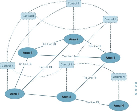
In this paper, we consider power system networks formed of distinct control areas which are interconnected via weak transmission lines referred to as tie-lines. Each area maintains a single nominal frequency across its geographical region and is comprised of either a single or a group of generators. In order for an area to maintain its frequency under load variations in the case of multiple generators, a local load frequency controller is used, distributed to the corresponding turbine-governing systems of each generating unit. The design of load frequency control (LFC) is based on a single-plant model which represents the sum of the generating units [1]. The area is responsible for meeting power demand of its own consumers, as well as of certain adjacent areas with which power exchange is normally scheduled for a contracted value. However, due to power load differentiation, the frequency of each area, along with the scheduled power exchange with its interconnected peers, may vary from their nominal value.
The rate of change of frequency (RoCoF) is related to the power system inertia and the active power mismatch. The relationship between inertia of a distinct area, RoCoF, and change in active power can be found in [2,3]. Virtually, synchronous machines have been the main source of system inertia, hence the area frequency is directly coupled to the rotational speed of the aggregated synchronous generators [2,4]. Traditionally, the prime mover of conventional thermal power stations and hydroelectric plants, along with the synchronous generators (typically of large inertia), act as smoothing (low-pass) filters on variations of electric loads and participate primarily in the frequency regulation of the area. In contrast, renewable energy generation units behave differently from conventional synchronous generators, mostly because they are connected through power electronic interfaces. In effect, these devices fully or partly can electrically decouple the generator from the grid [3], hence the coupling between the rotational speed of the generator and the system frequency is eliminated [5]. For this reason, unlike synchronous generators, inverter-connected generation units do not inherently contribute to the total system inertia [6]. Although control strategies for participation in frequency regulation by inverter-connected sources have been proposed in literature [7,8,9], such functions are rarely enabled in reality. Thus, the development of inverter-connected renewable energy sources introduces new challenges in the design of LFC, which is primarily performed by synchronous generating units due to their inherent capability to affect the RoCoF caused by active-power-imbalance events. Here, we focus on the design of LFC schemes with distributed pattern for multi-area power systems. In our model, we intentionally consider only synchronous generating units (thermal power stations, hydroelectric power plants) for the reasons outlined above. The violation of steady-state operation caused by active power imbalance is formulated as a feedback disturbance rejection problem of a large scale interconnected system.
LFC is one of the most challenging problems in multi-area power systems. An introduction to power systems design and LFC can be found in textbooks [2,10,11], while an overview of control strategies in the field of LFC problems has been discussed in [12,13]. Comprehensive literature surveys on the topic of LFC for diverse configurations of conventional and future smart power systems can be found in [14,15,16,17]. In typical situations, the geographical expanse and the mere complexity of the system resulting from dynamical couplings among areas make centralized control schemes either impossible or undesirable [18,19,20]. Hence, decentralized and distributed control is typically needed to ensure stable network operation. Analytical methods for designing a decentralized and distributed LFC have been presented in [21,22,23]. Robust decentralized control design methodologies have been presented in [24], where the authors propose two control schemes for LFC based on robust optimal control techniques and linear matrix inequalities (LMI). A rigorous and computationally efficient method, also based on the versatile formulation of LMI’s for robust decentralized control of multi-machine power systems, has been presented in [25].
A systematic methodology based on reachability for identifying the impact of potential cyber attacks in the Automatic Generation Control (AGC) of a two-area power system has been presented in [26]. Set-theoretic method for LFC design in the context of cyber-physical power systems can be found in [27], while in [28], the authors propose LFC design based on an anti-windup compensator, assuring stability of the closed-loop system even in cases of large load disturbance. Model predictive control has also attracted attention from the power system community in recent years due to its convenience in managing online disturbance rejection problems with state and input constraints, which is a highly desired feature in a multi-area power system control. Model predictive control with decentralized and distributed architecture for LFC design in interconnected power systems has been proposed in [29,30,31,32,33].
In this paper, we formulate the LFC of multi-area power systems as a large-scale optimal control problem in the absence of state and input constraints. An arbitrary number of identical areas is considered. The multi-area power system is represented as a multi-agent network composed of identical dynamically coupled linear time-invariant systems. These dynamical couplings can be expressed in a state-space form of a certain structure and represent interconnections between areas through tie-lines. In our case, each agent representing an area can produce LFC signals independently and is dynamically coupled with a certain number of its peers referred to as neighboring agents (areas) with whom it can exchange state information. Effectively, we assume that the topology of physical couplings (tie-lines) and the topology of information exchange among agents (areas) coincide and are described by the same graph.
Linear quadratic regulator (LQR) control design has been successfully utilized in frequency regulation problems, mostly due to large stability margins of its stabilizing solution, with the fundamental work of [34] being a benchmark approach to LQR-based LFC of multi-area power systems. Ever since, considerable research has been carried out on this topic; [35,36,37,38] represent some recent works. Over the past few years, there has been a renewal of interest in control of networks composed of a large number of interacting systems. The fundamental work of [39,40] in this field discusses distributed LQR design for a set of identical decoupled dynamical systems. Unfortunately, there is no documented distributed LQR-based approach to networked systems with dynamical couplings and, consequently, no distributed LQR-based LFC has been noticed in literature so far. The research of this paper motivated by the structure of a multi-area power system with dynamical couplings between interconnected areas, attempts to cover this particular gap in literature. We believe that this is the major contribution of our work the design description of which is summarized in the following paragraph.
We follow a top-down method to approximate a centralized LQR optimal controller by a distributed control scheme. It is shown that overall network stability is guaranteed via a stability test applied to a convex combination of Hurwitz matrices. The validity of this condition is consistent with the stability of a class of network interconnection structures which is identified. Sufficient condition for stability of convex combination of Hurwitz matrices can be found in [41]. Our approach was inspired by the powerful results proposed in [39]. Therein, the subsystems constituting the network are dynamically decoupled, and the stability of the distributed scheme designed relies on the stability margins of LQR control. A complementary distributed LQR method has also been proposed in [40], which consists of a bottom-up approach in which optimal interactions between self-stabilizing agents are defined so as to minimize an upper bound of the global LQR criterion. A major assumption of our work is that the dynamical models of each area are identical. Although this assumption may be unrealistic in practice, it simplifies the design problem considerably, which is especially hard due to the coupling terms appearing in the model. Future work will attempt to eliminate or relax this assumption. Preliminary results in this direction can be found in [42,43]. The simulation results presented in Section 6.2 were carried out under considerable perturbations and suggest that this hypothesis is valid and that our results can be extended to the non-identical case.
In this paper, our interest in distributed LFC arises from the necessity to avoid centralized schemes when these become computationally prohibitive. We wish to tackle the LFC problem of geographically sparse power grids following a distributed control approach, the main advantage of which is that it can replace the conventional centralized controller, which has high communication and processing costs and suffers from a single-point-of-failure drawback [23]. Faults caused by interconnection losses might give rise to an unacceptable frequency deviation and may accelerate a cascading failure event. The proposed distributed LFC controller is stabilizing even if tie-line interconnections and communication links are added to or removed from the overall system, as long as this does not violate the stability condition given in Section 4 and Section 5. This powerful feature gives integrity to the control subsystem of each area and enhances the resilience of the power system in the presence of interconnection variations. The main contributions of this paper are summarized as follows:
  • We propose a novel distributed-LQR algorithm for networked systems with dynamical couplings applied to LFC of large-scale multi-area power systems.
  • The control scheme is obtained by optimizing an LQR performance index with a tuning parameter which can be used to emphasize/de-emphasize relative state difference between interconnected areas. In effect, this parameter controls the magnitude of tie-line power exchange and frequency synchronization between interconnected areas.
  • Our approach enhances power system modularity and leads to a simple and verifiable stabilizability condition for a class of network topologies. Extensive simulations presented in this work support our conjecture that this stabilization criterion can be extended to more general LFC control network problems.
The remaining of the paper is organized in seven sections. In Section 2, preliminaries on graph theory are presented which are utilized in the control design contained in Section 4 and Section 5. In Section 3, we model a multi-area power system and describe the control problem of this paper. The main results of our work are presented in Section 4 and Section 5, which involve large-scale LQR problems. Section 6 presents simulation results, and Section 7 summarizes the main conclusions of the work. A discussion of the main results and suggestions for future work are also included in this section.

2. Preliminaries

A graph G is defined as the ordered pair G = ( V , E ) , where V is the set of nodes (or vertices) V = { 1 , , N } and E V × V the set of edges ( i , j ) with i V , j V . The degree d j of a graph vertex j is the number of edges which start from j. Let d m a x ( G ) denote the maximum vertex degree of the graph G . We denote by A ( G ) the ( 0 , 1 ) adjacency matrix of the graph G . In particular, the ( i j ) th element of A , A i j = 1 if ( i , j ) E i , j = 1 , , N , i j and zero otherwise. Let j N i if ( i , j ) E and i j . We call N i the neighborhood of node i. The adjacency matrix A ( G ) of undirected graphs is symmetric. We define the Laplacian matrix as L ( G ) = D ( G ) A ( G ) , where D ( G ) is the diagonal matrix of vertex degrees d i (also called the valence matrix). Let S ( L ( G ) ) = { λ 1 ( L ( G ) ) , , λ N ( L ( G ) ) } be the spectrum of the Laplacian matrix L associated with an undirected graph G arranged in nondecreasing semi-order. The following two results are standard.
Proposition 1.
Let G be a complete graph (with all possible edges) with N L vertices and L ( G ) be the corresponding Laplacian matrix. Then, S ( L ( G ) ) = { 0 , N L , , N L } .
Proposition 2.
Let A, B be matrices of appropriate dimensions and L be Laplacian matrix with spectrum S ( L ( G ) ) = { λ 1 ( L ( G ) ) , , λ N ( L ( G ) ) } . Then, the spectrum S ( I N A + L B ) can be reduced to i [ 1 : N ] S ( A + λ i B ) with λ i S ( L ) .
An extensive survey on the spectrum of the Laplacian matrix of graphs can be found in [44].

3. Multi-Area Power System Design

Power system networks can be decomposed into multiple distinct dynamical subsystems, referred to as control areas, each area having two primary characteristics; (1) It comprises of either a single generator or a group of generators, and (2) it maintains a single frequency across its geographical expanse. The areas are responsible for meeting the demand of their own consumers and are interconnected with each other through transmission lines, referred to as tie-lines, over which they exchange certain amount of power normally scheduled over a contracted value for each interconnection. In this paper, we consider a multi-agent representation of power systems where each agent/area has autonomous actuation capacity and is dynamically coupled with certain neighboring agents/areas with which it exchanges state-information. We assume that the topology of the physical links (tie-lines) and the communication scheme coincide. This multi-agent approach to multi-area power systems is illustrated in Figure 1, where physical structure of the network (solid lines) and communication links (dotted lines) are incorporated into one unified entity, representing a modern large-scale power system. The mapping of a cyber network to a physical grid, as shown in Figure 1, facilitates the data-exchange between the control subsystems of interconnected areas and allows for control schemes with distributed architecture. As mentioned earlier, each distinct area consists of a group of generating units, the aggregate power generation of which should match the demand of the consumers spanned across the geographical expanse covered by the corresponding area. The aggregate generation may comprise thermal power stations, hydroelectric plants, wind turbine farms, photovoltaic and battery storage power stations, and, in general, any type of conventional and renewable energy sources. In this work, to avoid further complications in designing distributed control schemes, the power generation of each area is limited to thermal and hydroelectric power stations.

3.1. Modeling

Let multi-area power system be composed of N areas the topology of which is modeled by undirected graph G = ( V , E ) . Each node i V represents an area and an edge ( i , j ) E between two nodes denotes interaction between the two nodes/areas. We note that the edge ( i , j ) of the graph determines coupling terms in the dynamics of area i and j and also indicates information exchange between node i and j. Let also all j V with j i such that ( i , j ) E be denoted by N i . In the sequel, all j N i are referred to as adjacent or neighboring nodes/areas to i. At steady-state operation the power sharing via tie-line interconnection between two areas i and j is denoted by P t i e , i , j and is given by:
P t i e , i , j = V i V j X i j sin ( δ i δ j ) .
Here, X i j is the reactance of the tie-line which connects the two areas, δ i , δ j represent the power angles of equivalent machines of area i and j, respectively, and V i , V j are the voltages at equivalent terminals of area i and j, respectively. Tie-line interconnection in a two-area system is depicted in Figure 2.
For small deviations of ( δ i , δ j ) from equilibrium ( δ i o , δ j o ) , the power flow deviation over tie-line i j from the nominal value is given by the linear equation:
Δ P t i e , i , j = T i j ( Δ δ i Δ δ j ) ,
where the synchronizing torque coefficient T i j = | V i | | V j | X i j cos ( δ i o δ j o ) , [10]. Notation Δ indicates deviation from steady-state operation conditions; differentiating (2) with respect to time results in:
Δ P ˙ t i e , i , j = K t i e , i , j Δ f i Δ f j ,
where K t i e , i , j = 2 π T i j is referred to as synchronization coefficient between area i and j, while Δ f i and Δ f j represent the frequency deviation of each area from their common nominal value, denoted here by f o . According to (3), the linearized dynamics of the total power inflow to the i-th area from all interconnected areas j N i , denoted by Δ P t i e , i is given by:
Δ P ˙ t i e , i = j N i K t i e , i , j ( Δ f i Δ f j ) .
The open-loop linearized dynamics of the i-th interconnected area is represented by a model widely used in literature [2,10], the block diagram of which is shown in Figure 3.
The total control signal of the i-th area is the sum of two components: Δ u t o t , i = Δ P f , i + Δ P C , i , namely the primary frequency control action, defined as Δ P f , i = 1 R i Δ f i and the AGC signal Δ P C , i to be designed. The first is a fixed static linear control law performed by the speed governor which is a regulating unit attached on the prime mover. Detailed description of this topic can be found in [2]. The static gain R i is referred to as speed droop or speed regulation and expresses the ratio of the frequency deviation Δ f i to a change in output generated power by Δ P G , i assuming the AGC signal Δ P C , i = 0 . A typical droop characteristic of a single generator actuated by primary frequency control is shown in Figure 4.
The signal Δ u t o t , i is assumed to be subjected to a component-wise saturation hard constraint of the form:
Δ u t o t , i , min Δ u t o t , i Δ u t o t , i , max ,
where Δ u t o t , i , max is taken greater than the maximum expected load deviation Δ P L , i , max ; otherwise, zero frequency deviation error is not guaranteed. Negative values of Δ u t o t , i allow for handling of negative values of Δ P L , i in case of load reduction. The rate of change of power generation due to the limitation of the thermal and mechanical movements in the generating unit of each area, as well as the speed governor dead band, are important issues in power system modeling. For simplicity, these constraints will be ignored in the linear stability analysis carried out in Section 4 and Section 5, and they will only be considered in simulation results in Section 6.
The corresponding state-space form of each area can be written as:
Δ f ˙ i Δ P ˙ G , i Δ P ˙ t i e , i = 1 T p , i K p , i T p , i K p , i T p , i K t , i R i T t , i 1 T t , i 0 0 0 0 A 1 , i Δ f i Δ P G , i Δ P t i e , i x i + j N i 0 0 K t i e , i , j ( Δ f i Δ f j ) E i + 0 K t , i T t , i 0 B u , i Δ P C , i u i + K p , i T p , i 0 0 B w , i Δ P L , i w i ,
for i = 1 , , N , where we have used the state-space differential equations with respect to block diagram Figure 3, along with (4). Note that E i corresponds to the dynamic coupling between the i-th area and its adjacent peers and gives rise to a state-space model of non-standard form. A standard state-space model for the complete network will be derived in the sequel. The variables Δ f i and Δ P t i e , i in the state-vector have been already defined; variable Δ P G , i in (6) is the deviation from equilibrium value of the electrical power generated by the aggregate generating units of each area and is taken equal to the mechanical power produced in the output of the turbines. All parameters involved in (6), along with basic power system terminology, are summarized in Table 1. The disturbance signal Δ P L , i denotes time-varying demand of the consumers of the i-th area and is assumed to correspond to unknown, piece-wise constant power load deviations with known upper and lower bounds. Here, we study the case where Δ P L , i , min Δ P L , i Δ P L , i , max for i = 1 , , N .

3.2. State-Augmentation for Integral Action

A well-established technique for tackling step-disturbances with zero steady-state error is to include integral action into the state-space model. For the i-th area, consider performance variable expressed as a summation of frequency deviation Δ f i multiplied by a bias factor β i and total tie-line power inflow Δ P t i e , i , or z i = β i Δ f i + Δ P t i e , i . This quantity is referred to as “Area Control Error” (ACE) and a usual choice for β i is D i + 1 R i , [10]. Parameters D i and R i are defined in Table 1. Take now z i = C z , i x i with x i given in (6) and C z , i = [ β i 0 1 ] and consider the augmented state-vector:
x a , i = x i z i .
The augmented state-space form of the i-th area can then be written as:
x ˙ a , i = A 1 , i 0 3 × 1 C z , i 0 x a , i + B u , i 0 u i + E i 0 + B w , i 0 w i ,
where A 1 , i , B u , i , E i and B w , i are as given in Equation (6). If the coupling term E i in Equation (8) is neglected, due to state-augmentation by the integral of the ACE signal of each area, a stabilizing control signal u i would lead automatically to zero steady-state frequency and tie-line power inflow deviations provided these are driven by step disturbances w i = Δ P L , i . However the term [ E i 0 ] involving state-coupling between the i-th area and its neighboring counterparts cannot be neglected, and therefore the disturbance rejection task for the complete network becomes more challenging.

3.3. Problem Statement

Possible power load change in the i-th area of an interconnected power system causes the electrical frequency f i to deviate from its nominal value. Due to interconnections among the areas through power transmission tie-lines and the dependence of the power exchange between the i-th and j-th area upon the respective difference Δ f i Δ f j , any power load deviation occurring in the i-th area will also affect the linked j-th area, causing a transient alternation in its frequency f j . Here, we formulate the LFC of multi-area power systems as a large-scale optimal control problem in the absence of state and input constraints. The special case of N identical areas is considered. The aggregate dynamics in this case can be represented by a state-space model of the form:
x ˜ ˙ = ( I N A 1 + L A 2 ) x ˜ + ( I N B u ) u ˜ + ( I N B w ) w ˜ .
Here, x ˜ = [ x a , 1 x a , N ] , u ˜ = [ u 1 u N ] , w ˜ = [ w 1 w N ] and:
A 1 = 1 T p K p T p K p T p 0 K t R T t 1 T t 0 0 0 0 0 0 β 0 1 0 , A 2 = 0 0 0 0 0 0 0 0 K t i e 0 0 0 0 0 0 0 , B u = 0 K t T t 0 0 , B w = K p T p 0 0 0 ,
where the subscript i has been neglected from all entries of A 1 , A 2 , B u , and B w since areas are assumed to have identical dynamics. The LQR design proposed in the next section is presented first from a general multi-agent perspective. This is then extended to the multi-area power system framework.

4. Large-Scale LQR for Dynamically Coupled Systems

Consider a network of N L dynamically coupled LTI systems referred to as agents. At local level, the dynamics of the i-th agent is represented in state-space form as:
x ˙ i = A 1 x i + A 2 j = 1 , j i N L ( x i x j ) + B u i , x 0 , i = x i ( 0 ) ,
where x i R n , u i R m are states and inputs of the i-th system, respectively. A complete graph (with all possible edges) G = ( V , E ) with Laplacian matrix L c is utilized to model the topology of the physical links among the agents. Node i V of G corresponds to local state x i , while edge ( i , j ) E corresponds to the x i x j term in (11). Now construct the aggregate state x ˜ R n N L and input vector u ˜ R m N L by stacking all state and input vectors, respectively, of all N L systems taken in ascending order depending on their label in graph G . The aggregate state-space of the network becomes:
x ˜ ˙ = A ˜ x ˜ + B ˜ u ˜ , x ˜ 0 = x ˜ ( 0 ) ,
with:
A ˜ = I N L A 1 + L c A 2 , B ˜ = I N L B .
Consider now LQR control problem for the network of N L coupled systems:
min u ˜ J ( u ˜ , x ˜ 0 ) s . t . x ˜ ˙ = A ˜ x ˜ + B ˜ u ˜ , x ˜ 0 = x ˜ ( 0 ) ,
where the cost function:
J ( u ˜ , x ˜ 0 ) = 0 x ˜ Q ˜ x ˜ + u ˜ R ˜ u ˜ d t ,
with:
Q ˜ = I N L Q 1 + L c Q 2   and   R ˜ = I N L R .
Here, the weighting matrices Q 1 = Q 1 0 and R = R > 0 penalize local states and inputs of each node, respectively, while the matrix Q 2 = Q 2 0 is chosen to weigh relative state differences between subsystems. The following stabilizability and observability assumptions guarantee a solution to LQR problem (14).
Assumption 1.
Let C 1 C 1 = Q 1 . The pair ( A 1 , B ) is stabilizable and ( A 1 , C 1 ) is observable.
Assumption 2.
Let C 12 C 12 = Q 1 + N L Q 2 . The pair ( A 1 + N L A 2 , B ) is stabilizable and ( A 1 + N L A 2 , C 12 ) is observable.
Under Assumption 1,2, problem (14) has a unique stabilizing solution u ˜ = K ˜ x ˜ , which gives finite performance index (15) equal to x ˜ 0 P ˜ x ˜ 0 . The optimal state-feedback gain K ˜ = R ˜ 1 B ˜ P ˜ , where P ˜ is the symmetric positive definite (s.p.d.) solution to the (large-scale) Algebraic Riccati Equation (ARE):
A ˜ P ˜ + P ˜ A ˜ P ˜ B ˜ R ˜ 1 B ˜ P ˜ + Q ˜ = 0 .
Due to special formulation of (14), K ˜ and P ˜ retain certain structure, which will prove essential for designing stabilizing distributed controllers in the next section. The specific structure of these matrices is proved in Theorem 1. In the following, we set X = B R 1 B .
Theorem 1.
Assume P ˜ is the s.p.d solution to (17) associated with the optimal solution to (14). Let P ˜ R n N L × n N L be decomposed into N L 2 blocks of dimension n × n , each denoted by P ˜ i j and referred to as the ( i , j ) -block of P ˜ . Then, the following statements hold.
I. 
j = 1 N L P ˜ i j = P where P = P 0 is the stabilizing solution to single-node ARE:
A 1 P + P A 1 P X P + Q 1 = 0 .
II. 
P ˜ i j = P ˜ k l = P ˜ 2 for all j i , l k where P ˜ 2 is symmetric matrix associated with the node-level ARE:
( A 1 + N L A 2 ) ( P N L P ˜ 2 ) + ( P N L P ˜ 2 ) ( A 1 + N L A 2 ) ( P N L P ˜ 2 ) X ( P N L P ˜ 2 ) + Q 1 + N L Q 2 = 0 .
Proof. 
First, we prove part I of the Theorem. The equations corresponding to the diagonal blocks of (17) are:
( A 1 + ( N L 1 ) A 2 ) P ˜ i i A 2 j = 1 j i N L P ˜ i j + P ˜ i i ( A 1 + ( N L 1 ) A 2 ) j = 1 j i N L P ˜ i j A 2 k = 1 N L P ˜ i k X P ˜ i k + Q 1 + ( N L 1 ) Q 2 = 0 ,
for i = 1 , , N L . Note that P ˜ i j = P ˜ j i due to symmetry of P ˜ in (17). Now let:
F i i = P ˜ i i + j = 1 j i N L P ˜ i j .
Substituting (21) to (20) gives:
( N L 1 ) ( A 2 F i i + F i i A 2 ) N L A 2 j = 1 j i N L P ˜ i j j = 1 j i N L P ˜ i j N L A 2
+ A 1 ( F i i j = 1 j i N L P ˜ i j ) + ( F i i j = 1 j i N L P ˜ i j ) A 1 k = 1 N L P ˜ i k X P ˜ i k + Q 1 + ( N L 1 ) Q 2 = 0 .
Using (21), the equations corresponding to the off-diagonal blocks of (17) can be written as:
( N L 1 ) ( A 2 P ˜ i j + P ˜ i j A 2 ) A 2 ( F i i k = 1 k i N L P ˜ i k ) ( F i i k = 1 k i N L P ˜ i k ) A 2 A 2 l = 1 l i l j N L P ˜ i l l = 1 l i l j N L P ˜ i l A 2
+ A 1 P ˜ i j + P ˜ i j A 1 k = 1 N L P ˜ i k X P ˜ k j Q 2 = 0 .
Summing up (23a) for all j i block-wise and adding this summation to (22a) gives:
( N L 1 ) A 2 F i i + F i i ( N L 1 ) A 2 ( N L 1 ) A 2 F i i F i i ( N L 1 ) A 2 N L A 2 j = 1 j i N L P ˜ i j j = 1 j i N L P ˜ i j N L A 2 + ( N L 1 ) A 2 j = 1 j i N L P ˜ i j + j = 1 j i N L P ˜ i j ( N L 1 ) A 2 + ( N L 1 ) A 2 k = 1 k i N L P ˜ i k + k = 1 k i N L P ˜ i k ( N L 1 ) A 2 ( N L 1 ) A 2 l = 1 l i l j N L P ˜ i l l = 1 l i l j N L P ˜ i l ( N L 1 ) A 2 = 0
where all the terms associated with A 2 cancel out. Summing up (23) over all j i block-wise and adding this summation to (22) gives:
A 1 F i i + F i i A 1 F i i X F i i + k = 1 k i N L P ˜ i k X F i i F k k + Q 1 = 0 .
Equation (25) has been established in Theorem 1 of [39]. It is true also here due to (24). Adding up (25) over all i = 1 , , N L , we get:
i = 1 N L A 1 F i i + F i i A 1 F i i X F i i + Q 1 = 0 ,
which is sum of N L identical ARE’s, i.e.,
N L ( A 1 F i i + F i i A 1 F i i X F i i + Q 1 ) = 0 .
Equation (21) implies F i i = i = 1 N L P ˜ i j which, along with (27), proves part I.
Since B ˜ , R ˜ are block diagonal and A ˜ , Q ˜ have a repetitive pattern, the ARE (17) can essentially be decomposed into N L identical equations. This implies that all P ˜ i j with i , j = 1 , , N L and j i are equal to each other. Let P ˜ 2 be symmetric matrix representing the off-diagonal blocks P ˜ i j of P ˜ . Setting P = F i i for i = 1 , , N L and P ˜ 2 = P ˜ i j for i , j = 1 , , N L and j i and substituting these matrices into (23) gives:
( N L 1 ) A 2 P ˜ 2 + ( N L 1 ) P ˜ 2 A 2 A 2 P P A 2 + ( N L 1 ) A 2 P ˜ 2 + ( N L 1 ) P ˜ 2 A 2 ( N L 2 ) A 2 P ˜ 2 ( N L 2 ) P ˜ 2 A 2 + A 1 P ˜ 2 + P ˜ 2 A 1 P ˜ 2 X ( P ( N L 1 ) P ˜ 2 ) ( P ( N L 1 ) P ˜ 2 ) X P ˜ 2 ( N L 2 ) P ˜ 2 X P ˜ 2 Q 2 = 0 ,
which after rearranging some terms and multiplying both sides by N L becomes:
( A 1 + N L A 2 ) ( N L P ˜ 2 ) + ( N L P ˜ 2 ) ( A 1 + N L A 2 ) + N L A 2 P + P N L A 2 ( N L P ˜ 2 ) X P P X ( N L P ˜ 2 ) ( N L P ˜ 2 ) X ( N L P ˜ 2 ) + N L Q 2 = 0 ,
or
( A 1 + N L A 2 ) ( N L P ˜ 2 ) + ( N L P ˜ 2 ) ( A 1 + N L A 2 ) + N L A 2 P + P N L A 2 + P X P ( P N L P ˜ 2 ) X ( P N L P ˜ 2 ) X + N L Q 2 = 0 .
Adding now (18) to (30) results in:
( A 1 + N L A 2 ) ( N L P ˜ 2 ) + ( N L P ˜ 2 ) ( A 1 + N L A 2 ) + ( A 1 + N L A 2 ) P + P ( A 1 + N L A 2 ) P X P + P X P ( P N L P ˜ 2 ) X ( P N L P ˜ 2 ) X + Q 1 + N L Q 2 = 0 ,
or
( A 1 + N L A 2 ) ( P N L P ˜ 2 ) + ( P N L P ˜ 2 ) ( A 1 + N L A 2 ) ( P N L P ˜ 2 ) X ( P N L P ˜ 2 ) + Q 1 + N L Q 2 = 0 ,
which proves part II. □
By assumption, the matrices R ˜ and B ˜ are selected block diagonal. Consequently, the state-feedback gain K ˜ = R ˜ 1 B ˜ P ˜ associated with the optimal solution to (14) retains the same structure with P ˜ . This leads to the following Corollary.
Corollary 1.
Assume K ˜ = R ˜ 1 B ˜ P ˜ is the optimal state-feedback gain obtained from the solution to (14) which gives minimum performance index x ˜ 0 P ˜ x ˜ 0 with P ˜ being the s.p.d solution to (17). Let K ˜ R m N L × n N L and P ˜ R n N L × n N L be decomposed into N L 2 blocks of dimension m × n and n × n denoted by K ˜ i j and P ˜ i j , respectively each referred to as ( i , j ) -block of the respective matrix. Then, the following are true;
I. 
P ˜ = I N L P L c P ˜ 2 .
II. 
j = 1 N L K ˜ i j = R 1 B P for i = 1 , , N L .
III. 
K ˜ i i = R 1 B P + ( N L 1 ) R 1 B P ˜ 2 for i = 1 , , N L .
IV. 
K ˜ i j = R 1 B P ˜ 2 for i , j = 1 , , N L and j i .
V. 
K ˜ = I N L R 1 B P + L c R 1 B P ˜ 2 .
Theorem 1 states that due to special formulation of the cost function (15) and the structure of the aggregate state-space form (12), the large-scale LQR problem (14) under Assumption 1,2 can effectively be reduced to finding the solution of two node-level ARE’s. This feature may be highly beneficial for problems involving networks, the topology of which is modeled by graph with an excessively large number of vertices ( N L ) .
Applying the stabilizing optimal state-feedback control u ˜ = K ˜ x ˜ to (12) results in a closed-loop matrix, which is Hurwitz and is written as:
A c l = I N L ( A 1 X P ) + L c ( A 2 + X P ˜ 2 ) .
Due to Proposition 2, the spectrum of A c l can be decomposed into:
S ( A c l ) = i = 1 N L S A 1 X P + λ c , i ( A 2 + X P ˜ 2 ) ,
where λ c , i { 0 , N L , , N L } .
Remark 1.
The matrix A 1 X P + α N L ( A 2 + X P ˜ 2 ) is Hurwitz for α = 0 and α = 1 .
In the sequel, we require that:
Condition 1.
The matrix A 1 X P + α N L ( A 2 + X P ˜ 2 ) is Hurwitz for all α [ 0 , 1 ] .
Condition 1 states that all convex combinations of two Hurwitz matrices,
μ A ¯ 1 + ( 1 μ ) A ¯ 2   with   μ [ 0 , 1 ] ,
are Hurwitz, where A ¯ 1 = A 1 X P + N L ( A 2 + X P ˜ 2 ) and A ¯ 2 = A 1 X P . Sufficient conditions for Hurwitz stability of convex combination of Hurwitz matrices can be found in Theorem 2 . 2 in [41]. In essence, Condition 1 characterizes a class of LQR problems (14) which admit of solutions for which the Condition 1 holds. This will be used later for the design of distributed stabilizing controllers. For a given selection of weighting matrices ( Q 1 , Q 2 , R ) of the LQR problem (14), the validity of Condition 1 can be verified by searching for a symmetric positive definite matrix P ¯ for which the following LMI,
( A ¯ 1 P ¯ + P ¯ A ¯ 1 ) 0 n × n 0 n × n 0 n × n ( A ¯ 2 P ¯ + P ¯ A ¯ 2 ) 0 n × n 0 n × n 0 n × n P ¯ > 0 ,
is feasible. Obviously, if matrix P ¯ exists then premultiplying and postmultiplying (36) by [ μ I n 1 μ I n 0 n × n ] and [ μ I n 1 μ I n 0 n × n ] , respectively, for μ [ 0 , 1 ] leads to Lyapunov inequality:
( μ A ¯ 1 + ( 1 μ ) A ¯ 2 ) P ¯ + P ¯ ( μ A ¯ 1 + ( 1 μ ) A ¯ 2 ) < 0 ,
which admits of a solution P ¯ = P ¯ > 0 . This demonstrates that μ A ¯ 1 + ( 1 μ ) A ¯ 2 is a Hurwitz matrix for all μ [ 0 , 1 ] . Alternatively, the stability of μ A ¯ 1 + ( 1 μ ) A ¯ 2 can be examined via a simple graphical test by plotting the eigenvalue with the maximum real part of the matrix μ A ¯ 1 + ( 1 μ ) A ¯ 2 for μ [ 0 , 1 ] .

Distributed LQR Design for Dynamically Coupled Systems

Let sparse network be formed of N identical and dynamically coupled LTI systems. We note here that the index N differs from N L employed for networks modeled by complete graph in the previous section, and in the sequel, we use index N to refer to schemes with sparse structure. Let the couplings among the systems be modeled by graph G N = ( V , E ) with Laplacian matrix L N . The neighborhood of the i-th system is denoted by N i V and comprises all j V with j i , for which ( i , j ) E . Let the dynamics at local level of the i-th system be:
x ˙ i = A 1 x i + A 2 j N i ( x i x j ) + B u i , x 0 , i = x i ( 0 ) ,
where x i R n and u i R m . The aggregate state-space of the network becomes:
x ˜ ˙ = A ˜ x ˜ + B ˜ u ˜ , x ˜ 0 = x ˜ ( 0 ) ,
where x ˜ R n N , u ˜ R m N and:
A ˜ = I N A 1 + L N A 2 , B ˜ = I N B .
Note that the Laplacian matrix L N in (40) does not necessarily correspond to a complete graph in contrast to (13) and generically the matrix A ˜ in (40) is sparse. A stabilizing distributed controller for (39) is constructed in the following Theorem. For convenience, we set X = B R 1 B .
Theorem 2.
Consider a network of N coupled systems with dynamics described in (38). The network topology is modeled by graph G N with Laplacian matrix L N . Let λ N be the maximum eigenvalue of L N and denote by d m a x the smallest integer which is greater than or equal to λ N . Consider LQR problem (14) for N L = d m a x , define P and P ˜ 2 via (18) and (19), respectively, and assume Condition 1 is true. Define also distributed state-feedback gain:
K ^ = I N R 1 B P + L N R 1 B P ˜ 2 .
Then, the closed-loop matrix,
A c l = I N ( A 1 X P ) + L N ( A 2 + X P ˜ 2 ) ,
is Hurwitz.
Proof. 
Consider the spectrum S ( A c l ) = S ( I N ( A 1 X P ) + L N ( A 2 + X P ˜ 2 ) ) . Let V N I n be state-space transformation, where V N R N × N is an orthogonal matrix whose columns consist of the eigenvectors of L N . In the transformed coordinates, A ¯ c l = I N ( A 1 X P ) + Λ N ( A 2 + X P ˜ 2 ) , where Λ N = d i a g ( 0 , λ 2 , , λ N ) with λ N d m a x . The spectrum of A ¯ c l is:
S ( A ¯ c l ) = i = 1 N ( A 1 X P + λ i ( A 2 + X P ˜ 2 ) ) ,
where λ i for i = 1 , , N are the eigenvalues of L N . Condition 1 holds, hence ( A 1 X P ) + α d m a x ( A 2 + X P ˜ 2 ) is Hurwitz for all α [ 0 , 1 ] . Consequently, A ¯ c l is also Hurwitz since λ i [ 0 , d m a x ] for all i = 1 , , N . This proves the Theorem. □
Remark 2.
For a time-varying graph G ( t ) = ( V , E ( t ) ) with fixed number of vertices ( N ) and time-varying edges the maximum eigenvalue of the time-varying Laplacian matrix L ( t ) is bounded by 2 N . Consequently, solving (14) for N L = 2 N and assuming Condition 1 holds leads to a distributed controller K ^ , which stabilizes the network for all possible couplings among the N systems. Naturally, this does not imply stability of switching between stable network interconnections.

5. Large-Scale LQR for LFC

In this section, we consider LQR problem (14) for a multi-area power system. Recall that we denote by N L the number of areas of power network, the topology of which is modeled by complete graph and by N the number of areas corresponding to sparse networks. Let the aggregate state-space model of N L -area power system be written as:
x ˜ ˙ = ( I N L A 1 + L c A 2 ) x ˜ + ( I N L B u ) u ˜ + ( I N L B w ) w ˜ ,
where x ˜ = [ x a , 1 x a , N L ] , u ˜ = [ u 1 u N L ] , w ˜ = [ w 1 w N L ] with x a , i , u i , w i for i = 1 , , N L defined in (8) and:
A 1 = 1 T p K p T p K p T p 0 K t R T t 1 T t 0 0 0 0 0 0 β 0 1 0 , A 2 = 0 0 0 0 0 0 0 0 K t i e 0 0 0 0 0 0 0 , B u = 0 K t T t 0 0 , B w = K p T p 0 0 0 .
Parameters in ( A 1 , A 2 , B u , B w ) can be found in Table 1. In view of Assumption 1, LQR problem (14) for A ˜ = I N L A 1 + L c A 2 and B ˜ = I N L B u with ( A 1 , A 2 , B u ) given in (10) initially fails to admit a solution since (18) cannot be solved. This stems from the fact that the pair ( A 1 , B u ) has an uncontrollable mode at the origin, and the realization (44) is non-minimal. The non-minimality is due to a redundant equation related to the sum of the total power inflow Δ P t i e , i to each area, which equals zero or i = 1 N L Δ P t i e , i = 0 . Now, we show how to reformulate the system matrices and derive a stabilizing controller for the network.
Define permutation matrix:
T = 1 0 0 0 0 1 0 0 0 0 0 1 0 0 1 0 ,
where T = T = T 1 and consider Kalman decomposition of the pair ( A 1 , B u ) applying state-space transformation T x a , i for i = 1 , , N L . Let the system matrices ( A ¯ 1 , A ¯ 2 , B ¯ u , B ¯ w ) = ( T A 1 T , T A 2 T , T B u , T B w ) in the new coordinates be written as:
A ¯ 1 = 1 T p K p T p 0 K p T p K t R T t 1 T t 0 0 β 0 0 1 0 0 0 0 , A ¯ 2 = 0 0 0 0 0 0 0 0 0 0 0 0 K t i e 0 0 0 , B ¯ u = 0 K t T t 0 0 , B ¯ w = K p T p 0 0 0 ,
where B ¯ u = B u , B ¯ w = B w . The controllable part of ( A ¯ 1 , B ¯ u ) is denoted by ( A c , B c ) with:
A c = 1 T p K p T p 0 K t R T t 1 T t 0 β 0 0 , B c = 0 K t T t 0 .
The zero in the ( 4 , 4 ) entry of A ¯ 1 stands for the uncontrollable mode at the origin of ( A 1 , B u ) . Now, construct perturbation matrix:
Energies 12 02664 i002
for e < 0 with | e | sufficiently small and define:
Energies 12 02664 i003
where A 12 = [ K t R T t 0 1 ] and a 21 = [ K t i e 0 0 ] . Since e < 0 , the pair ( A 1 e , B u ) is stabilizable. According to Theorem 1, LQR problem (14) with parameters ( A 1 e , A 2 e , B u , Q 1 , Q 2 , R ) is reduced to two node-level ARE:
A 1 e P e + P e A 1 e P e X P e + Q 1 = 0
, ( A 1 e + N L A 2 e ) ( P e N L P ˜ 2 e ) + ( P e N L P ˜ 2 e ) ( A 1 e + N L A 2 e ) ( P e N L P ˜ 2 e ) X ( P e N L P ˜ 2 e )
+ Q 1 + N L Q 2 = 0 ,
where P e , P ˜ 2 e are e-dependent and X = B u R 1 B u . Note that the solution P e N L P ˜ 2 e to ARE (52) remains invariant under e-perturbation. Theorem 3, next, summarizes the method of solving large-scale LQR problem (14) with one uncontrollable mode at the origin.
Theorem 3.
Consider N L -area power system with aggregate state-space form given as in (44). Consider Kalman decomposition of ( A 1 , B u ) and define ( A ¯ 1 , A ¯ 2 , B ¯ u , B ¯ w ) given in (47). Choose e < 0 with | e | sufficiently small and define perturbed matrices A 1 e , A 2 e as given in (50). Solving LQR problem (14) with parameters ( A 1 e , A 2 e , B u , Q 1 , Q 2 , R ) and defining P e and P ˜ 2 e from (51) and (52), respectively, leads to the following argument: the matrix,
A ¯ 1 X P e + α ( N L A ¯ 2 + X P ˜ 2 e ) ,
I. 
is Hurwitz for α = 1 .
II. 
has n 1 eigenvalues in the left-half-plane and one at the origin for α = 0 .
Proof. 
In view of the special structure of A 1 e and A 2 e , it can easily be seen that:
A ¯ 1 + N L A ¯ 2 = A 1 e + N L A 2 e .
Due to (52), the matrix A 1 e + N L A 2 e X P e + N L X P ˜ 2 e is Hurwitz and because of (54) the matrix A ¯ 1 + N L A ¯ 2 X P e + N L X P ˜ 2 e is also Hurwitz. This proves part I.
Now, let the matrix P e in (51) be decomposed into blocks of appropriate dimensions according to the Kalman decomposition (48). Then, ARE (51) can be written as:
A c A 12 0 3 e P 11 e P 12 e P 12 e P 22 e + P 11 e P 12 e P 12 e P 22 e A c A 12 0 3 e P 11 e P 12 e P 12 e P 22 e B c 0 R 1 B c 0 P 11 e P 12 e P 12 e P 22 e + Q 11 Q 12 Q 12 Q 22 = 0 .
The first diagonal block of (55) gives:
A c P 11 e + P 11 e A c P 11 e B c R 1 B c P 11 e + Q 11 = 0 ,
and implies that the matrix A c B c R 1 B c P 11 e is Hurwitz where the symmetric positive definite matrix P 11 e does not depend on parameter e. The two remaining blocks P 12 e and P 22 e of P e are e-dependent and given by:
P 12 e = ( A c P 11 e B c R 1 B c + e I n 1 ) 1 ( P 11 e A 12 + Q 12 ) ,
P 22 e = 1 2 e [ ( P 12 e B c R 1 B c 2 A 12 ) P 12 e Q 22 ] .
The matrix A c P 11 e B c R 1 B c + e I n 1 in (57) is invertible since A c B c R 1 B c P 11 e is Hurwitz and e < 0 . Now, the closed-loop matrix A 1 e B u R 1 B u P e is Hurwitz and can be written as:
A 1 e B u R 1 B u P e = A c B c R 1 B c P 11 e A 12 B c R 1 B c P 12 e 0 3 e .
Since (59) is in canonical form, its spectrum can be decomposed in:
S ( A 1 e B u R 1 B u P e ) = S ( A c B c R 1 B c P 11 e ) e .
Setting e = 0 in (60) proves the Theorem. □
Similarly to Condition 1, we impose the following stability requirement.
Condition 2.
The matrix A ¯ 1 X P e + α ( N L A ¯ 2 + X P ˜ 2 e ) is Hurwitz for all α ( 0 , 1 ] .
In the next paragraph, we propose distributed stabilizing LFC controllers for multi-area power systems with sparse topology based on Condition 2.

5.1. Distributed LQR-Based LFC

Let undirected graph G N = ( V , E ) with Laplacian matrix L N ( G N ) models the interconnection topology of a multi-area power system formed of N identical areas with aggregate state-space form written as:
x ˜ ˙ = ( I N A 1 + L N A 2 ) x ˜ + ( I N B u ) u ˜ + ( I N B w ) w ˜ .
The matrices A 1 , A 2 , B u , and B w are given as in (45). The aggregate vectors x ˜ , u ˜ , and w ˜ are constructed by stacking the augmented state-vector x a , i , input-vector u i , and disturbance-vector w i , respectively, shown in (8) of each area with ascending order depending on graph G N . Now, define perturbation matrix:
E = 0 0 0 0 0 0 0 0 0 0 e 0 0 0 0 0 ,
where e < 0 and | e | sufficiently small, and also define perturbed matrices A 1 e and A 2 e as:
A 1 e = A 1 + E , A 2 e = A 2 1 N L E ,
where N L is as defined in Theorem 2. A distributed LFC controller for (61) is constructed next, in Theorem 4.
Theorem 4.
Consider power system of N identical areas with network topology modeled by graph G N with Laplacian matrix L N and aggregate state-space form given by (61). Let λ N be the maximum eigenvalue of L N and denote by d m a x the smallest integer which is greater than or equal to λ N . Set N L = d m a x , specify e < 0 with | e | sufficiently small and define perturbed matrices A 1 e and A 2 e as in (63). Consider LQR problem (14) for N L = d m a x perturbed systems ( A 1 e , A 2 e , B u ) , define P e and P ˜ 2 e via (51) and (52), respectively, and assume Condition 2 holds. Define also distributed state-feedback gain:
K ^ = I N R 1 B u P e + L N R 1 B u P ˜ 2 e .
Then, the closed-loop matrix of the original system,
A c l = I N ( A 1 X P e ) + L N ( A 2 + X P ˜ 2 e ) ,
has 3 N 1 eigenvalues in the left-hand-plane and one at the origin.
The proof follows similar arguments stated for proving Theorem 2 and is omitted here. The conclusions as far as the stability of the network is concerned still hold, even if the controllability Assumption 1 is no longer valid. The distributed state-feedback gain (64) can be used for stabilizing the network despite the fact that the closed-loop matrix (65) has a single eigenvalue at the origin. This mode corresponds to the trivial differential equation i = 1 N L Δ P ˙ t i e , i = 0 , which implies 0 ˙ = 0 and can be easily derived via an appropriate state-space transformation.
In the following section, the distributed LQR controller constructed above is employed to drive the LFC of a six-area power system. We show that network stability is guaranteed for a class of tie-line interconnection structures via a single tuning of the LFC controller. In the simulations, we consider three different interconnection schemes. We also include certain input and state constraints in the linear model of each area in order to assess the stability margins of the proposed control scheme. A robust stability test has also been carried out as a separate case study involving parametric uncertainties in the parameters of each area. We stress here that robust stability and nonlinear analysis are beyond the scope of this paper. Nonlinearities and parameter perturbations considered in the next section are only used for simulation purposes where the performance of the proposed control scheme is also tested under more intense conditions.

6. Simulation Case Studies

We consider a power system of six identical areas, the parameters of which are summarized in Table 1. Three interconnection schemes are considered; each graph shown in Figure 5a–c, with corresponding Laplacian matrix given in (66), models the network topology of one of the three schemes ( S 1 , S 2 , S 3 ) , respectively.
L 1 = 2 1 0 0 1 0 1 2 1 0 0 0 0 1 3 1 0 1 0 0 1 2 1 0 1 0 0 1 2 0 0 0 1 0 0 1 , L 2 = 1 0 0 0 1 0 0 1 1 0 0 0 0 1 2 1 0 0 0 0 1 3 1 1 1 0 0 1 2 0 0 0 0 1 0 1 , L 3 = 3 0 1 0 1 1 0 1 0 1 0 0 1 0 1 0 0 0 0 1 0 2 1 0 1 0 0 1 3 1 1 0 0 0 1 2 .
In the simulations, one scenario is considered in which the areas are assumed to be subjected to step disturbances. These represent power load variations of the consumers of each area and are depicted in Figure 6. For the control design, we also assume that there is a communication cyber-layer, the topology of which is identical with this of the tie-line interconnection scheme considered. The distributed LFC controller designed in Theorem 4 was tested in three case studies, which are summarized below:
  • We test closed-loop stability of topology S 1 , S 2 , and S 3 , respectively, applying LFC controller derived by solving a single LQR problem. This stability test is performed for two different tunings of the LQR performance index. The transients of frequency and total power inflow of the linear model of each area is compared to the corresponding responses, including saturation hard constraint on the total input signal of each area.
  • We consider parametric uncertainty in the linear model of each area, and we show closed loop stability of topology S 2 for two different tunings of the LFC controller. Perturbations have been carried out on the following parameters: turbine time constant ( T t , i ) , area time constant ( T p , i ) of each area, respectively, and tie-line coefficient ( K t i e , i , j ) of each tie-line interconnection.
  • For a certain tuning of the LFC controller, we demonstrate frequency recovery for topology S 1 , S 2 , and S 3 , respectively, including generation rate constraint (GRC) and saturation hard constraint on the total input signal of each area.

6.1. Case Study 1

Block representation of the linear dynamics of each control area at local level is given in Figure 3. The corresponding augmented state-space form of each area is shown in (8), where the integral of the ACE signal has also been included in the state-vector. We construct the collective state-space of the network as in (61), where matrices A 1 , A 2 , B u , and B w are given in (45). The Laplacian matrix L corresponds to one of those given in (66) according to the topology considered. Parameter values are given in Table 1. The distributed LQR controller presented in Section 5.1 is proposed here to drive the AGC signal Δ P C , i of each area. The control objective is to meet the load demand at each area shown in Figure 6 and recover the nominal operating conditions of each area for three possible interconnections. Stabilizing distributed state-feedback controller is constructed as follows.
The maximum eigenvalue of each matrix ( L 1 , L 2 , L 3 ) in (66) is 4 . 3028 , 4 . 3028 , and 4 . 3928 , respectively. We take the smallest integer denoted by d m a x which is greater or equal to the maximum of these ( 4 . 3928 ), i.e., d m a x = 5 . We select perturbation parameter e = 0 . 01 , and we alter matrices A 1 and A 2 to A 1 e and A 2 e , respectively, according to (63). We solve optimal problem (14) for N L = d m a x = 5 systems with matrices ( A 1 e , A 2 e , B u ) for two different selections of the weights Q ˜ , R ˜ . In the first, Q ˜ = I 5 Q 1 , with Q 1 = d i a g ( 100 , 10 , 10 , 5000 ) and R ˜ = I 5 100 , while in the second, R ˜ is kept the same and Q ˜ = I 5 Q 1 + L 5 Q 2 , where Q 2 = 200 Q 1 and L 5 is Laplacian matrix corresponding to complete graph (all possible edges) with 5 nodes. The matrix Q 2 penalizes the relative state-difference ( x i x j ) between neighboring areas in (15). We evaluate P e and P ˜ 2 e from (51), (52), and we define the respective K = R 1 B u P e and K 2 = R 1 B u P ˜ 2 e state-feedback gains for each tuning. These are:
K = 2502 . 857 1 . 203 1 . 757 7 . 071 K 2 = 342 . 491 0 . 104 0 . 225 0 . 000
for the first tuning where Q 2 = 0 and:
K = 2502 . 857 1 . 203 1 . 757 7 . 071 K 2 = 12084 . 071 2 . 356 6 . 374 43 . 329
for the case where Q 2 = 200 Q 1 . Note that K = R 1 B u P e is the same for both cases since P e is the solution to a single node-level ARE with parameters ( A 1 e , B u , Q 1 , R ) . We also test the validity of Condition 2, which can be seen to hold. Figure 7 displays the real part of the eigenvalue of the matrix ( A 1 B u R 1 B u P e ) + α d m a x ( A 2 + B u R 1 B u P ˜ 2 e ) with the maximum real part with α [ 0 , 1 ] for both tuning choices. In essence, this implies stable operation of the network under both control schemes for all possible interconnections corresponding to Laplacian matrices with maximum eigenvalue bounded by d m a x .
At network level, the distributed stabilizing controller K ^ takes the form:
K ^ = I 6 K + L s K 2 ,
where L s , s = 1 , 2 , 3 , is given in (66) according to the topology. Node-wise, the AGC signal at each area is derived from:
Δ P C , i = K x i + K 2 j N i ( x i x j ) ,
with i = 1 , , 6 , j i and j N i . In effect, each area requires local state and state-information from its neighboring areas be accessible for measuring in order to construct its control signal. In the following simulations, we show the transients of frequency and total power inflow of each area resulting from the corresponding power demand deviation Δ P L , i , i = 1 , , 6 of each area. Comparison with the response of the corresponding model of each area which includes saturation hard constraint on the total input signal of each area is also illustrated in the simulation results. Block representation of each area with saturating input constraint is shown in Figure 8, where the symmetric saturator models the lower and upper bound of the magnitude of the total control signal of each area. Here, we consider 220 [ MW ] Δ u t o t , i 220 [ MW ] , i = 1 , , 6 .
Figure 9, Figure 10, Figure 11 and Figure 12 show the transient response of frequency and total power inflow deviation, respectively, of each area from the equilibrium operation for two control schemes given in (67), (68). Stable operation is guaranteed and the nominal working conditions for all three interconnection schemes are recovered via both LFC control choices. For the given choices of weighting matrices ( Q 1 , Q 2 , R ) , this is guaranteed from the validity of Condition 2, which was checked graphically in Figure 7. Note also, the magnitude of the total power flow over the tie-lines is significantly limited in the case where the controller is designed as in (68). This stems from the large weighting matrix Q 2 selection in the performance index (15). In this case, since the relative state-difference between neighboring areas is highly penalized, the areas tend to acquire same frequencies deviations during the transients (see Figure 11), thus the total power flow over the tie-lines given in (4) is kept low. Comparing Figure 10 and Figure 12, the same behavior is observed for the case in which saturating input constraint is included in the model of each area. Despite the strong nonlinearity introduced by the saturator, total power inflow of each area is significantly reduced when the relative state-difference ( x i x j ) is penalized heavily in the LQR performance index. This powerful feature to control the magnitude of tie-line power exchange enhances the applicability of the proposed controller and might prove highly beneficial for networks composed of weak tie-line interconnections.

6.2. Case Study 2

To assess the stability margins of the LFC controller constructed in the previous case study, we introduce uncertain parameters in the model of each area, and we carry out simulations for the interconnection topology S 2 shown in Figure 5b. Both tunings of the LQR performance index considered in the previous section are also employed here. We consider parametric uncertainties in: turbine time constant T t , i , area time constant T p , i and tie-line coefficient K t i e , i , j for i , j = 1 , , 6 and j N i . The perturbation magnitude of each parameter is shown in Table 2.
The frequency and total power inflow deviation of each area driven by step disturbances (Figure 6) are depicted in Figure 13, Figure 14, Figure 15 and Figure 16. The robustness of the proposed distributed LQR-based LFC scheme is validated, and it can be seen that stable operation is maintained even for magnitude of parametric uncertainties taken equal to 30 % .

6.3. Case Study 3

In this simulation study, the linear model of each area is augmented by saturation hard constraint on the total control signal and generation rate constraint (GRC). The first is formulated as hard input constraint and is taken equal to this considered in the first case study, 220 [ MW ] Δ u t o t , i 220 [ MW ] , i = 1 , , 6 . The second constraint (GRC) can be cast as state constraint imposed on the state variable Δ P G , i , = 1 , , 6 . Here, we consider GRC equal to 10 % of the power base of each area per minute (i.e., 3.4 [MW/s]). The augmented block diagram of each area is depicted in Figure 17.
Each area is subjected to step disturbances shown in Figure 6. The three tie-line interconnection schemes depicted in Figure 5 are considered in the simulations. In this case study, in order to construct the proposed LFC controller, the weighting matrices of the LQR performance index have been chosen according to Bryson’s rule [45]. For a standard LQR problem with weights ( Q , R ) , this rule specifies that Q and R are taken diagonal with diagonal entries defined as:
Q i i = 1 ( x i , m a x ) 2   and   R i i = 1 ( u i , m a x ) 2 ,
where | x i , m a x | and | u i , m a x | represent the maximum required values of the state and control variables, respectively. Here, the matrices ( Q 1 , Q 2 , R ) are selected as: Q 1 = d i a g ( 1 0 . 001 2 , 1 450 2 , 1 200 2 , 1 100 2 ) , Q 2 = d i a g ( 1 0 . 1 2 , 1 50 2 , 1 400 2 , 1 5000 2 ) and R = 10000 350 2 . The frequency transient of the closed-loop system of each area is illustrated in Figure 18.
As it can be seen, the same LFC controller stabilizes the network for topology S 1 , S 2 , and S 3 and nominal frequency for each area is recovered. The frequency transient in this case has become considerably slower than in previous studies due to the state constraint GRC, which significantly limits the rate of power generation (3.4 [MW/s]). Despite the strong nonlinearities introduced by the input and state constraint, the closed-loop stability is maintained via the proposed LFC controller.

7. Conclusions

A stabilizing distributed state-feedback LFC scheme for multi-area power systems was proposed based on the solution of a large-scale LQR optimal problem under the assumption that the dynamic models of each area are identical. This method has originally been proposed in [39] for the decoupled case and was extended here to include couplings between the subsystems representing power system areas. First, a fully centralized controller was designed which was subsequently substituted by a distributed state-feedback gain with sparse structure. The control scheme was obtained by optimizing an LQR performance index with a tuning parameter utilized to emphasize/de-emphasize relative state difference between interconnected areas. We showed that this parameter controls the magnitude of tie-line power exchange and frequency synchronization between interconnected areas. Our approach enhances power system modularity and leads to a simple and verifiable stabilizability condition for a class of network topologies. Extensive simulations presented in this work support our conjecture that this stabilization criterion can be extended to more general LFC control network problems. The assumption of identical dynamics is clearly restrictive but simplifies the design problem considerably and leads to the derivation of a stability condition which can be easily tested. Attempts to eliminate or relax this assumption will be the topic of future work. Preliminary results in this direction can be found in [42,43]. The simulation results in Section 6.2 carried out under considerable perturbations suggest that this hypothesis is valid and that our results can be extended to the non-identical case.

Author Contributions

All authors have contributed equally to the derivation of the results of this work. All authors have approved the publication of this paper.

Funding

L. Dritsas acknowledges financial support from the Special Account for Research of ASPETE through the funding program “Strengthening research of ASPETE faculty members”.

Conflicts of Interest

The authors declare no conflict of interest.

References

  1. Iracleous, D.P.; Alexandridis, A.T. A multi-task automatic generation control for power regulation. Electr. Power Syst. Res. 2005. [Google Scholar] [CrossRef]
  2. Kundur, P. Power System Stability And Control; McGraw-Hill, Inc.: London, UK, 1993. [Google Scholar]
  3. Tielens, P.; Van Hertem, D. The relevance of inertia in power systems. Renew. Sustain. Energy Rev. 2016, 55, 999–1009. [Google Scholar] [CrossRef]
  4. Ulbig, A.; Borsche, T.S.; Andersson, G. Impact of low rotational inertia on power system stability and operation. IFAC Proc. Vol. 2014, 47, 7290–7297. [Google Scholar] [CrossRef]
  5. Masood, N.A.; Modi, N.; Yan, R. Low inertia power systems: Frequency response challenges and a possible solution. In Proceedings of the 2016 Australasian Universities Power Engineering Conference (AUPEC), Brisbane, Australia, 25–28 September 2016. [Google Scholar]
  6. Tielens, P.; van Hertem, D. Grid Inertia and Frequency Control in Power Systems with High Penetration of Renewables. In Proceedings of the Young Researchers Symposium in Electrical Power Engineering, Delft, The Netherlands, 16–17 April 2012. [Google Scholar]
  7. Žertek, A.; Verbič, G.; Pantoš, M. A novel strategy for variable-speed wind turbines’ participation in primary frequency control. IEEE Trans. Sustain. Energy 2012, 3, 791–799. [Google Scholar] [CrossRef]
  8. Attya, A.B.T.; Hartkopf, T. Control and quantification of kinetic energy released by wind farms during power system frequency drops. IET Renew. Power Gener. 2013, 7, 210–224. [Google Scholar] [CrossRef]
  9. Oshnoei, A.; Khezri, R.; Muyeen, S.; Blaabjerg, F. On the Contribution of Wind Farms in Automatic Generation Control: Review and New Control Approach. Appl. Sci. 2018, 8, 1848. [Google Scholar] [CrossRef]
  10. Bevrani, H. Robust Power System Frequency Control; Springer: Berlin/Heidelberg, Germany, 2010. [Google Scholar]
  11. Ma, J. Power System Wide-Area Stability Analysis and Control; Wiley: Hoboken, NJ, USA, 2018. [Google Scholar]
  12. Shayeghi, H.; Shayanfar, H.A.; Jalili, A. Load frequency control strategies: A state-of-the-art survey for the researcher. Energy Convers. Manag. 2009. [Google Scholar] [CrossRef]
  13. Pappachen, A.; Peer Fathima, A. Critical research areas on load frequency control issues in a deregulated power system: A state-of-the-art-of-review. Renew. Sustain. Energy Rev. 2017, 72, 163–177. [Google Scholar] [CrossRef]
  14. Pandey, S.K.; Mohanty, S.R.; Kishor, N. A literature survey on load-frequency control for conventional and distribution generation power systems. Renew. Sustain. Energy Rev. 2013. [Google Scholar] [CrossRef]
  15. Shankar, R.; Pradhan, S.R.; Chatterjee, K.; Mandal, R. A comprehensive state of the art literature survey on LFC mechanism for power system. Renew. Sustain. Energy Rev. 2017, 76, 1185–1207. [Google Scholar] [CrossRef]
  16. Haes Alhelou, H.; Hamedani-Golshan, M.E.; Zamani, R.; Heydarian-Forushani, E.; Siano, P. Challenges and opportunities of load frequency control in conventional, modern and future smart power systems: A comprehensive review. Energies 2018, 11, 2497. [Google Scholar] [CrossRef]
  17. Brinda, M.D.; Suresh, A.; Rashmi, M. A literature survey on LFC in a deregulated electricity environment. World Rev. Sci. Technol. Sustain. Dev. 2018. [Google Scholar] [CrossRef]
  18. Scattolini, R. Architectures for distributed and hierarchical Model Predictive Control—A review. J. Process Control 2009, 19, 723–731. [Google Scholar] [CrossRef]
  19. Langbort, C.; Chandra, R.S.; D’Andrea, R. Distributed control design for systems interconnected over an arbitrary graph. IEEE Trans. Autom. Control 2004, 49, 1502–1519. [Google Scholar] [CrossRef]
  20. Olfati-Saber, R. Flocking for Multi-Agent Dynamic Systems:Algorithms and Theory. IEEE Trans. Autom. Control 2006, 51, 1–20. [Google Scholar] [CrossRef]
  21. Andreasson, M.; Dimarogonas, D.V.; Sandberg, H.; Johansson, K.H. Distributed PI-control with applications to power systems frequency control. In Proceedings of the 2014 American Control Conference, Portland, OR, USA, 4–6 June 2014. [Google Scholar]
  22. Andreasson, M.; Dimarogonas, D.V.; Johansson, K.H.; Sandberg, H. Distributed vs. In centralized power systems frequency control. In Proceedings of the 2013 European Control Conference (ECC), Zurich, Switzerland, 17–19 July 2013; pp. 3524–3529. [Google Scholar] [CrossRef]
  23. Bidram, A.; Lewis, F.L.; Davoudi, A. Distributed control systems for small-scale power networks: Using multiagent cooperative control theory. IEEE Control Syst. 2014, 34, 56–77. [Google Scholar]
  24. Rerkpreedapong, D.; Hasanović, A.; Feliachi, A. Robust load frequency control using genetic algorithms and linear matrix inequalities. IEEE Trans. Power Syst. 2003. [Google Scholar] [CrossRef]
  25. Siljak, D.D.; Stipanovic, D.M.; Zecevic, A.I. Robust Decentralized Turbine/Governor Control. IEEE Trans. Power Syst. 2002, 17, 715–722. [Google Scholar] [CrossRef]
  26. Esfahani, P.M.; Vrakopoulou, M.; Margellos, K.; Lygeros, J. Cyber Attack in a Two-Area Power System : Impact Identification using Reachability. In Proceedings of the 2010 American Control Conference (ACC 2010), Baltimore, MD, USA, 30 June–2 July 2010; pp. 962–967. [Google Scholar]
  27. Kontouras, E.; Tzes, A.; Dritsas, L. Set-theoretic detection of data corruption attacks on cyber physical power systems. J. Mod. Power Syst. Clean Energy 2018, 6, 872–886. [Google Scholar] [CrossRef] [Green Version]
  28. Dritsas, L.; Kontouras, E.; Kitsios, I.; Tzes, A. Aggressive Control Design for Electric Power Generation Plants. In Proceedings of the 2018 26th Mediterranean Conference on Control and Automation (MED), Zadar, Croatia, 19–22 June 2018. [Google Scholar]
  29. Venkat, A.N.; Hiskens, I.A.; Rawlings, J.B.; Wright, S.J. Distributed MPC strategies with application to power system automatic generation control. IEEE Trans. Control Syst. Technol. 2008, 16, 1192–1206. [Google Scholar] [CrossRef]
  30. Mohamed, T.H.; Bevrani, H.; Hassan, A.A.; Hiyama, T. Decentralized model predictive based load frequency control in an interconnected power system. Energy Convers. Manag. 2011, 52, 1208–1214. [Google Scholar] [CrossRef]
  31. Wang, D.; Glavic, M.; Wehenkel, L. Comparison of centralized, distributed and hierarchical model predictive control schemes for electromechanical oscillations damping in large-scale power systems. Int. J. Electr. Power Energy Syst. 2014. [Google Scholar] [CrossRef]
  32. Ma, M.; Zhang, C.; Liu, X.; Chen, H. Distributed Model Predictive Load Frequency Control of the Multi-Area Power System after Deregulation. IEEE Trans. Ind. Electron. 2017. [Google Scholar] [CrossRef]
  33. Ma, M.; Chen, H.; Liu, X.; Allgöwer, F. Distributed model predictive load frequency control of multi-area interconnected power system. Electr. Power Energy Syst. 2014, 62, 289–298. [Google Scholar] [CrossRef]
  34. Fosha, C.E.; Elgerd, O.I. The Megawatt-Frequency Control Problem: A New Approach Via Optimal Control Theory. IEEE Trans. Power Appar. Syst. 1970. [Google Scholar] [CrossRef]
  35. Pandey, S.K.; Mohanty, S.R.; Kishor, N.; Catalão, J.P.S. An Advanced LMI-Based-LQR Design for Load Frequency Control of an Autonomous Hybrid Generation System. In Proceedings of the Doctoral Conference on Computing, Electrical and Industrial Systems, Costa de Caparica, Portugal, 15–17 April 2013; Springer: Berlin/Heidelberg, Germany, 2013; Volume 394, pp. 371–381. [Google Scholar] [CrossRef]
  36. Shankar, G.; Lakshmi, S.; Nagarjuna, N. Optimal load frequency control of hybrid renewable energy system using PSO and LQR. In Proceedings of the 2015 International Conference on Power and Advanced Control Engineering (ICPACE), Bangalore, India, 12–14 August 2015; pp. 195–199. [Google Scholar] [CrossRef]
  37. Devi, P.S.; Santhi, R.V.; Pushpalatha, D.V. Introducing LQR-fuzzy technique with dynamic demand response control loop to load frequency control model. IFAC-PapersOnLine 2016, 49, 567–572. [Google Scholar] [CrossRef]
  38. Shahalami, S.H.; Farsi, D. Analysis of Load Frequency Control in a restructured multi-area power system with the Kalman filter and the LQR controller. AEU Int. J. Electron. Commun. 2018, 86, 25–46. [Google Scholar] [CrossRef]
  39. Borrelli, F.; Keviczky, T. Distributed LQR design for identical dynamically decoupled systems. IEEE Trans. Autom. Control 2008, 53, 1901–1912. [Google Scholar] [CrossRef]
  40. Deshpande, P.; Menon, P.P.; Edwards, C.; Postlethwaite, I. Sub-optimal distributed control law with H2 performance for identical dynamically coupled linear systems. IET Control Theory Appl. 2012, 6, 2509–2517. [Google Scholar] [CrossRef]
  41. Białas, S. A sufficient condition for Hurwitz stability of the convex combination of two matrices. Control Cybern. 2004, 33, 109–112. [Google Scholar]
  42. Vlahakis, E.E.; Halikias, G.D. Distributed LQR Methods for Networks of Non-Identical Plants. In Proceedings of the 2018 IEEE Conference on Decision and Control (CDC), Miami Beach, FL, USA, 17–19 December 2018; pp. 6145–6150. [Google Scholar]
  43. Vlahakis, E.E.; Halikias, G.D. Model-Matching type-methods and Stability of Networks consisting of non-Identical Dynamic Agents. IFAC-PapersOnLine 2018, 51, 426–431. [Google Scholar] [CrossRef]
  44. Mohar, B. The Laplacian spectrum of graphs. Graph Theory Comb. Appl. 1991, 2, 12. [Google Scholar]
  45. Hespanha, J.P. Undergraduate Lecture Notes on LQG/LQR Controller Design; UCBS (University of California, Santa Barbara): Santa Barbara, CA, USA, 2005. [Google Scholar]
Figure 1. Tie-line interconnections (solid lines) and communication scheme (dotted lines) in large-scale multi-area power system.
Energies 12 02664 g001
Figure 2. Tie-line interconnection of two-area system.
Energies 12 02664 g002
Figure 3. Single block representation of the i-th interconnected area.
Energies 12 02664 g003
Figure 4. Droop characteristic.
Energies 12 02664 g004
Figure 5. Three different tie-line interconnection schemes of six control areas.
Energies 12 02664 g005
Figure 6. Power demand deviation Δ P L , i for i = 1 , , 6 .
Energies 12 02664 g006
Figure 7. Stability test and validity of Condition 2.
Energies 12 02664 g007
Figure 8. Single block representation of the i-th interconnected area with saturation hard constraint on the total input signal.
Energies 12 02664 g008
Figure 9. Frequency transients of the six-area power system for three tie-line interconnection schemes ( S 1 , S 2 , S 3 ) . Zero penalty on the relative state-difference between interconnected areas. Solid lines depict transients of the linear model; dashed lines depict transients of the model with saturator (Figure 8).
Energies 12 02664 g009
Figure 10. Total power inflow response of the six-area power system for three tie-line interconnection schemes ( S 1 , S 2 , S 3 ) . Zero penalty on the relative state-difference between interconnected areas. Solid lines depict transients of the linear model; dashed lines depict transients of the model with saturator (Figure 8).
Energies 12 02664 g010
Figure 11. Frequency transients of the six-area power system for three tie-line interconnection schemes ( S 1 , S 2 , S 3 ) . Large penalty on relative state-difference between interconnected areas. Solid lines depict transients of the linear model; dashed lines depict transients of the model with saturator (Figure 8).
Energies 12 02664 g011
Figure 12. Total power inflow response of the six-area power system for three tie-line interconnection schemes ( S 1 , S 2 , S 3 ) . Large penalty on relative state-difference between interconnected areas. Solid lines depict transients of the linear model; dashed lines depict transients of the model with saturator (Figure 8).
Energies 12 02664 g012
Figure 13. Frequency deviation Δ f i response for i = 1 , , 6 , topology S 2 , control tuning with Q 2 = 0 , uncertain parameters.
Energies 12 02664 g013
Figure 14. Frequency deviation Δ f i response for i = 1 , , 6 , topology S 2 , control tuning with Q 2 = 200 Q 1 , uncertain parameters.
Energies 12 02664 g014
Figure 15. Total power inflow deviation Δ P t i e , i response for i = 1 , , 6 , topology S 2 , control tuning with Q 2 = 0 , uncertain parameters.
Energies 12 02664 g015
Figure 16. Total power inflow deviation Δ P t i e , i response for i = 1 , , 6 , topology S 2 , control tuning with Q 2 = 200 Q 1 , uncertain parameters.
Energies 12 02664 g016
Figure 17. Single block representation of the i-th interconnected area with saturation hard constraint on the total input signal and nonlinear turbine model with GRC.
Energies 12 02664 g017
Figure 18. Frequency transients of the six-area power system for three tie-line interconnection schemes ( S 1 , S 2 , S 3 ) . Input and state constraints are included in the model of each area (Figure 17). Selection of weighting matrices according to Bryson’s rule.
Energies 12 02664 g018
Table 1. Parameters and power system terminology.
Parameter, SymbolValueUnits
Nominal Frequency, f o 50Hz
Power Base, P B , i 2000MW
Load Dependency Factor, D i 16 . 66 MW/Hz
Speed Droop, R i 1 . 2 × 10 3 Hz/MW
Generator Inertia Gain, H i 5s
Turbine Static Gain, K t , i 1MW/MW
Turbine Time Constant, T t , i 0 . 3 s
Area Static Gain, K p , i 0 . 06 Hz/MW
Area Time Constant, T p , i 24s
Tie-line Coefficient, K t i e , i 1090MW/Hz
Table 2. Parametric uncertainties in T t , i , T p , i and K t i e , i , j , i = 1 , , 6 , j N i .
Energies 12 02664 i001

