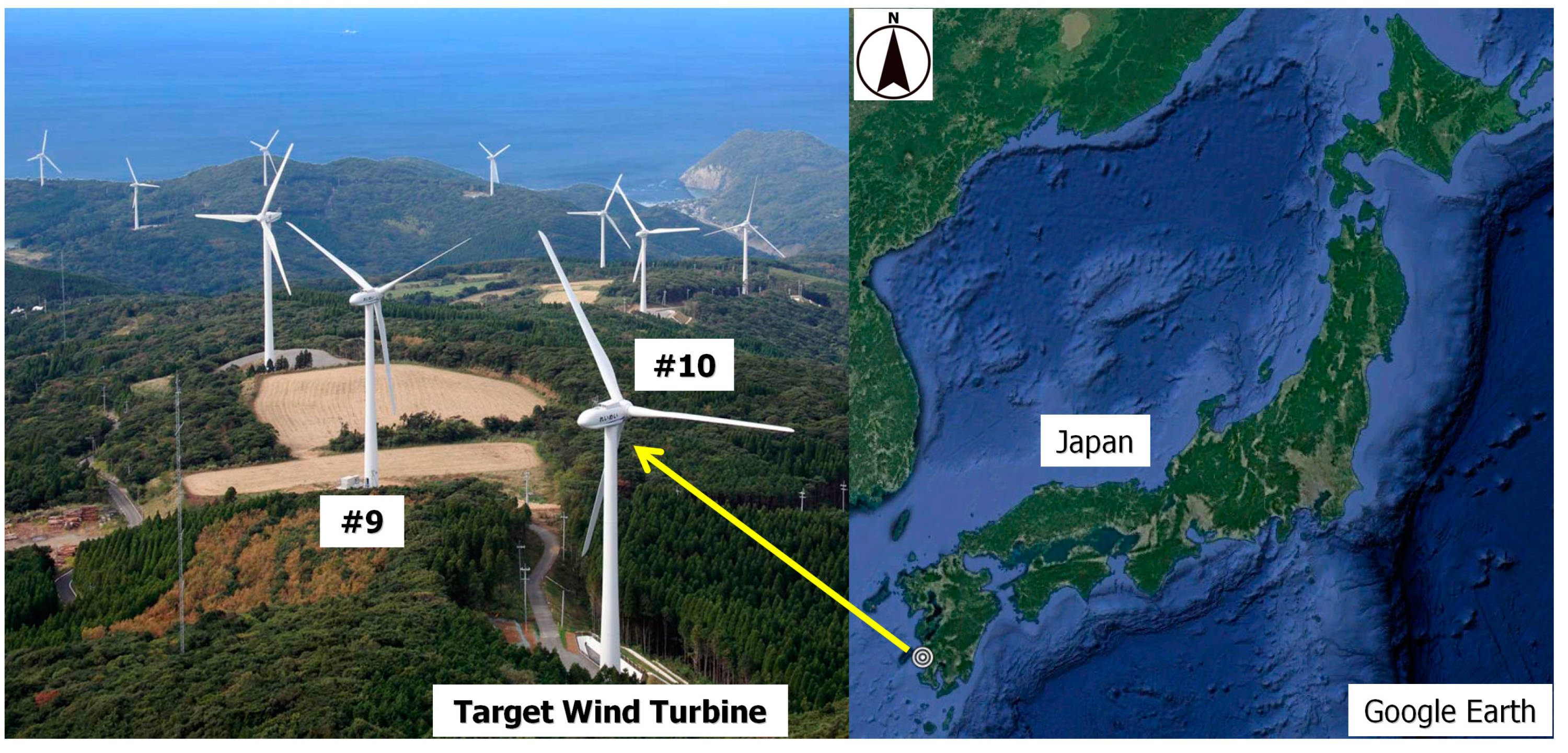
Figure 1.
Map of the Kushikino Reimei Wind Farm and the surrounding area.
Figure 1.
Map of the Kushikino Reimei Wind Farm and the surrounding area.
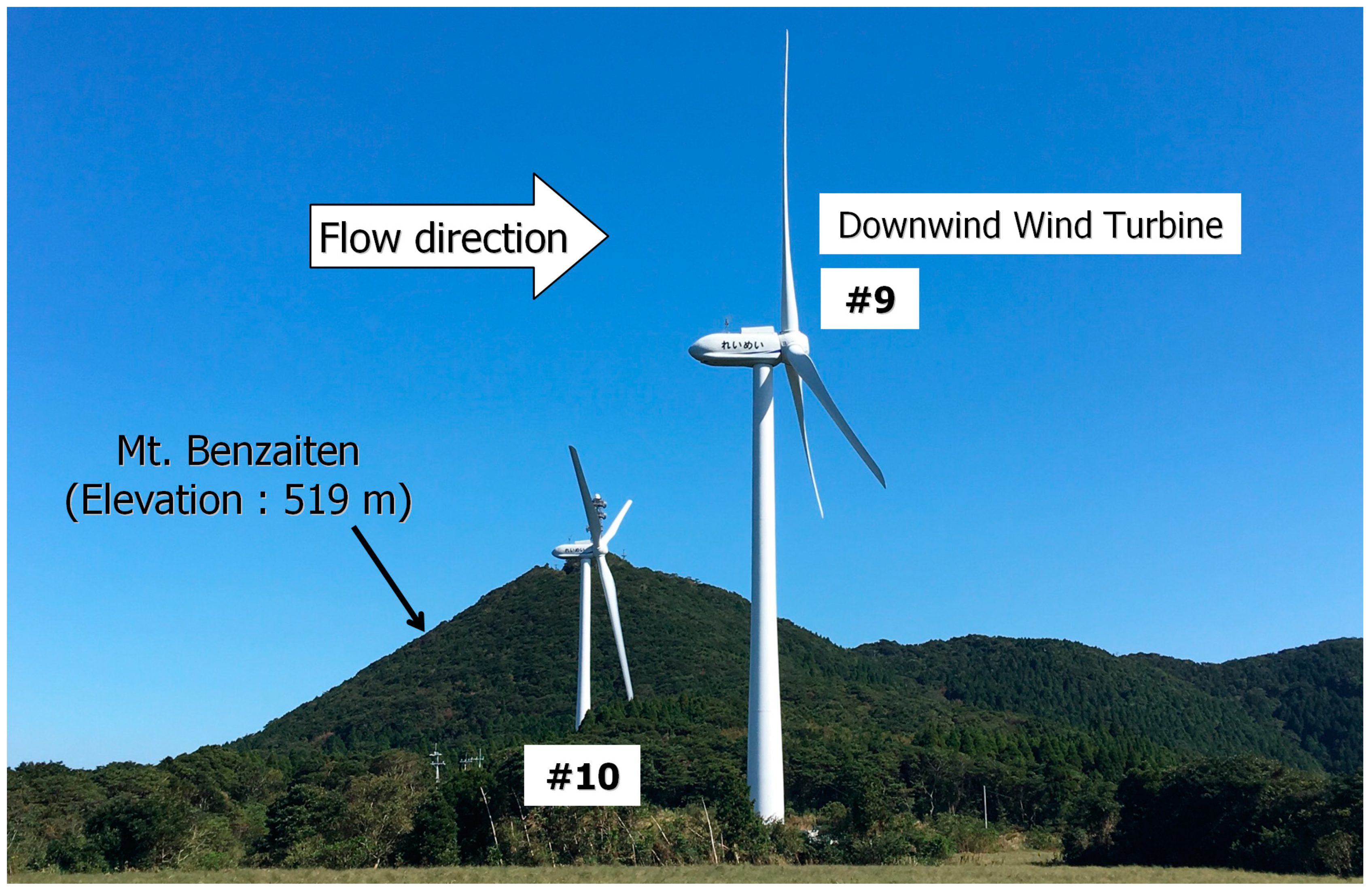
Figure 2.
Photo of wind turbine #10.
Figure 2.
Photo of wind turbine #10.
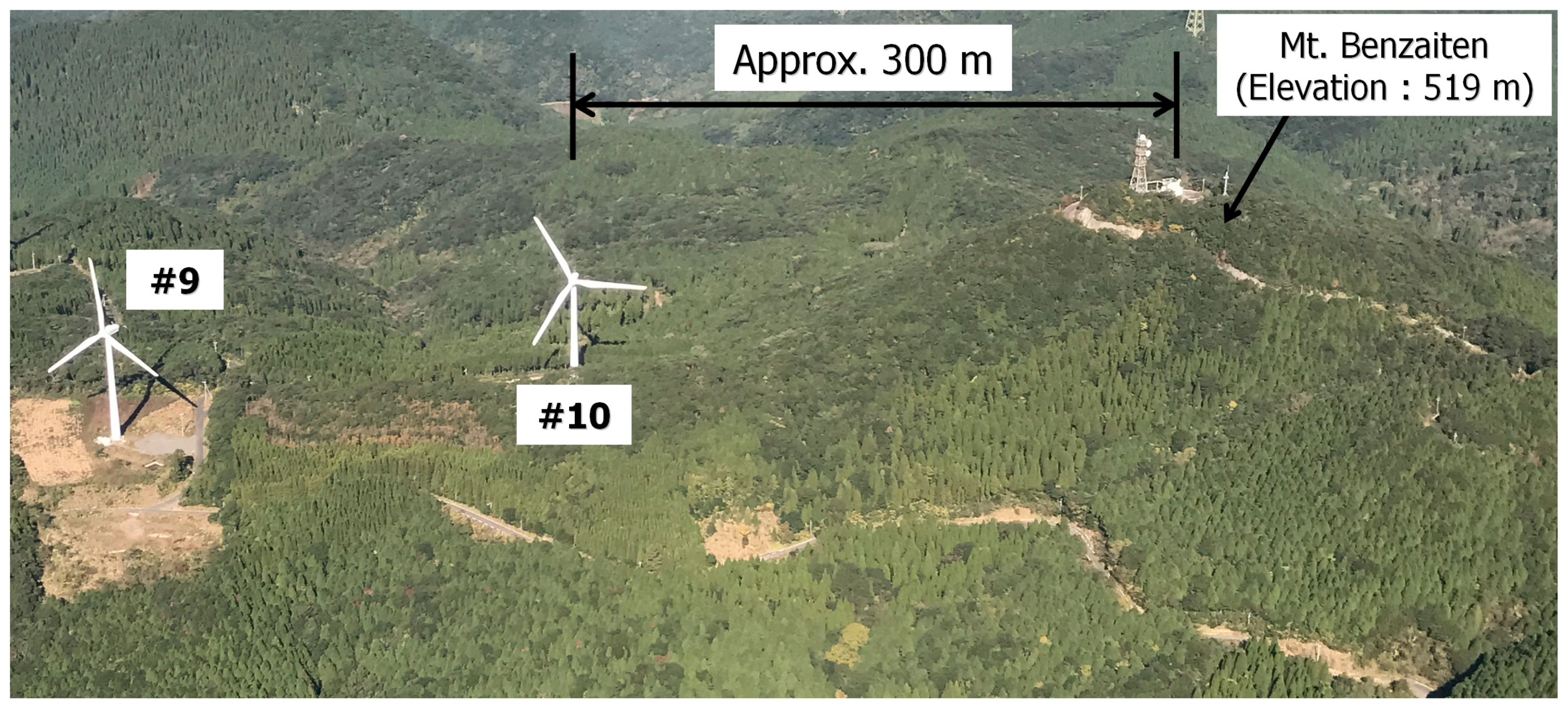
Figure 3.
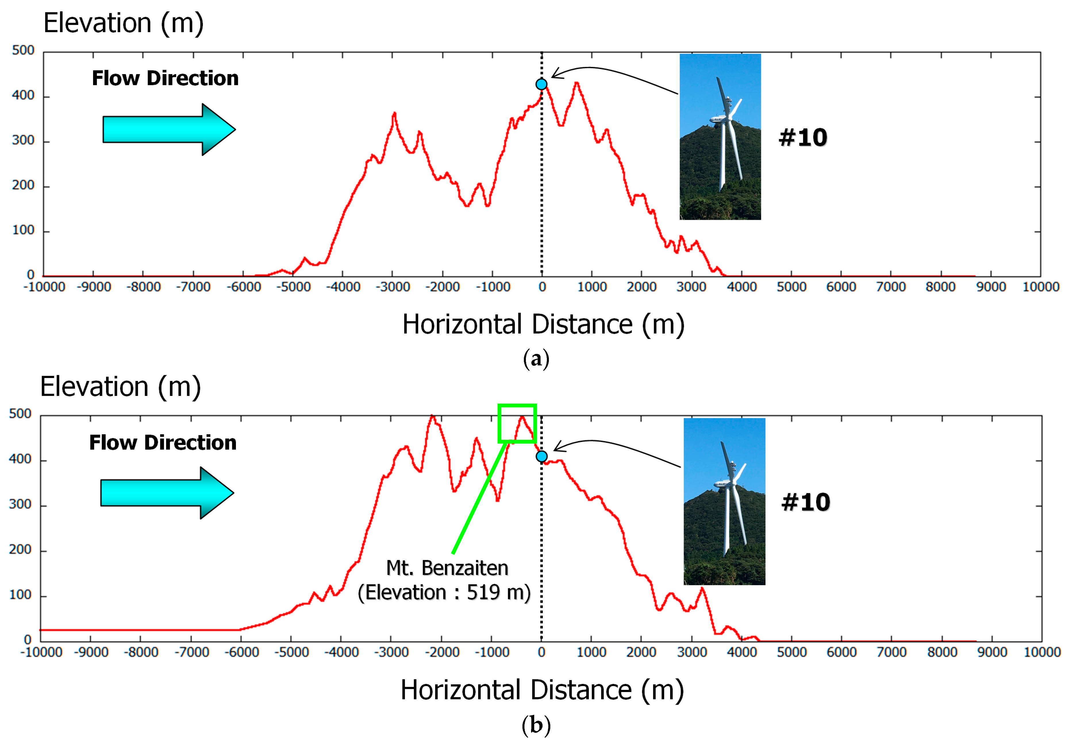
Relative locations of Mt. Benzaiten (elevation 519 m) and wind turbine #10.
Figure 3.
Relative locations of Mt. Benzaiten (elevation 519 m) and wind turbine #10.
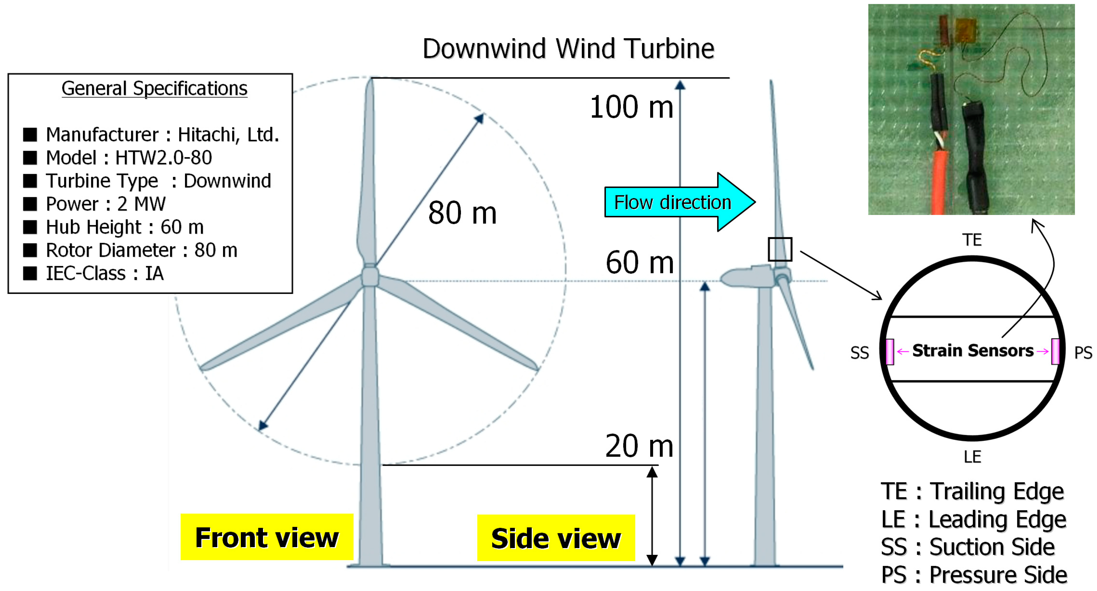
Figure 4.
Outline of a wind turbine.
Figure 4.
Outline of a wind turbine.
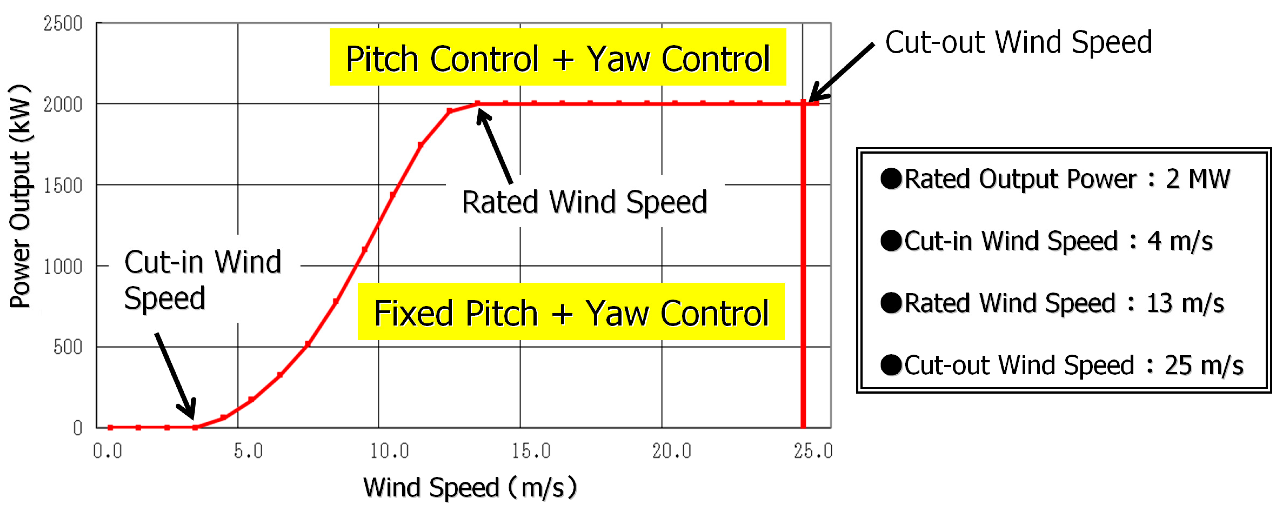
Figure 5.
Power curve of a wind turbine.
Figure 5.
Power curve of a wind turbine.
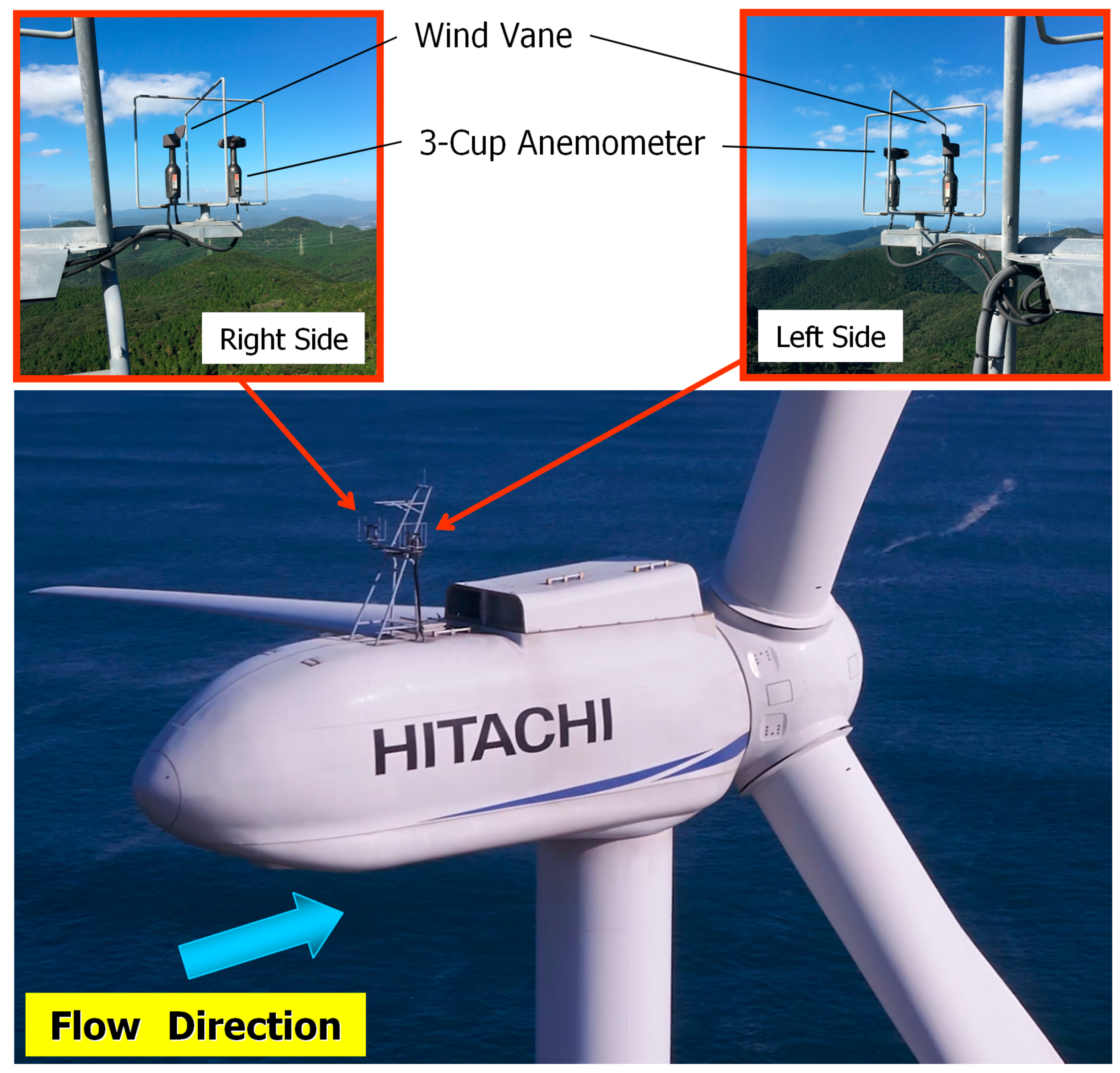
Figure 6.
Nacelle propeller-vane anemometer.
Figure 6.
Nacelle propeller-vane anemometer.
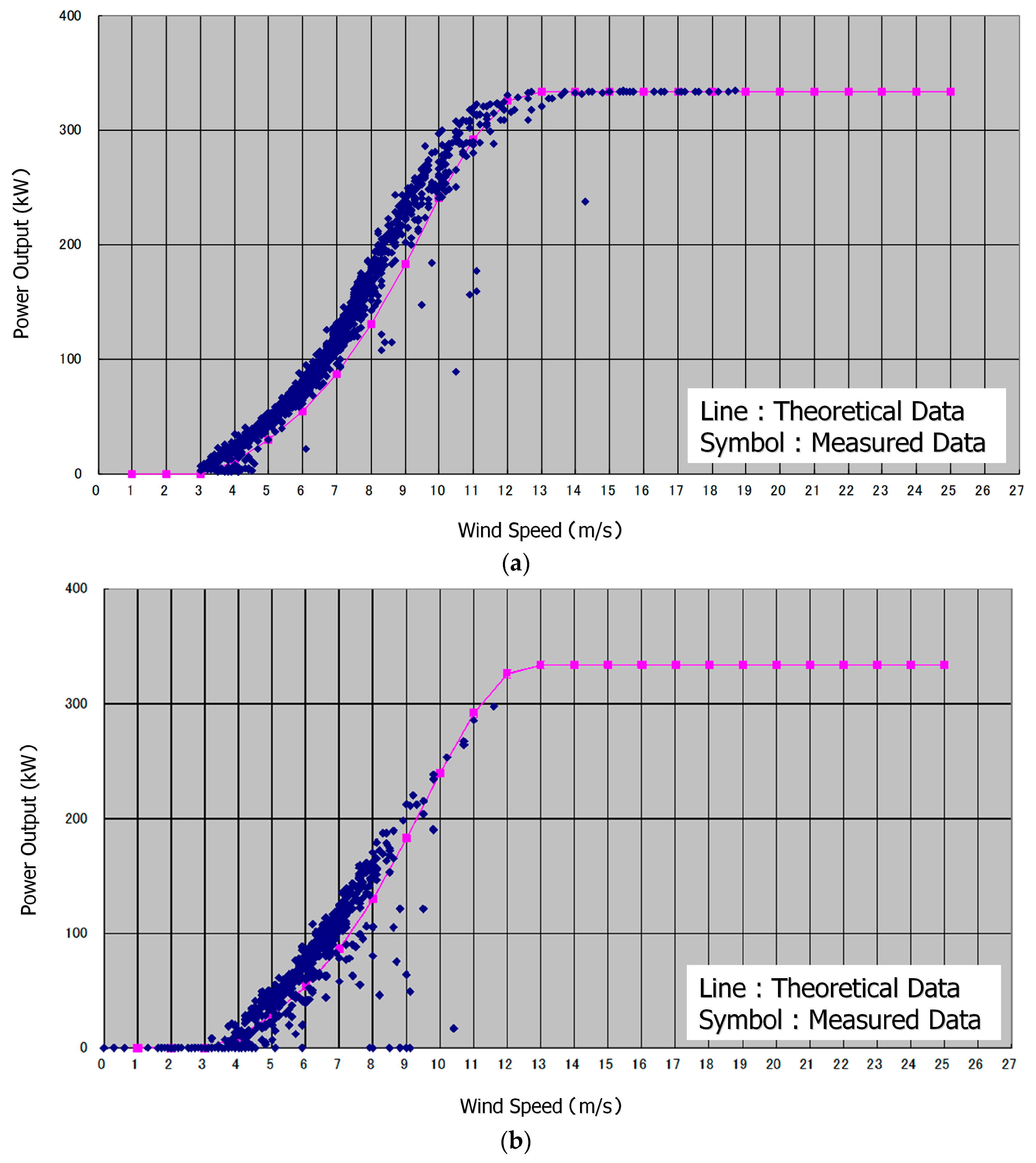
Figure 7.
Comparison between theoretical data and measured data for wind turbine #10. (a) Northerly wind. (b) Easterly wind.
Figure 7.
Comparison between theoretical data and measured data for wind turbine #10. (a) Northerly wind. (b) Easterly wind.
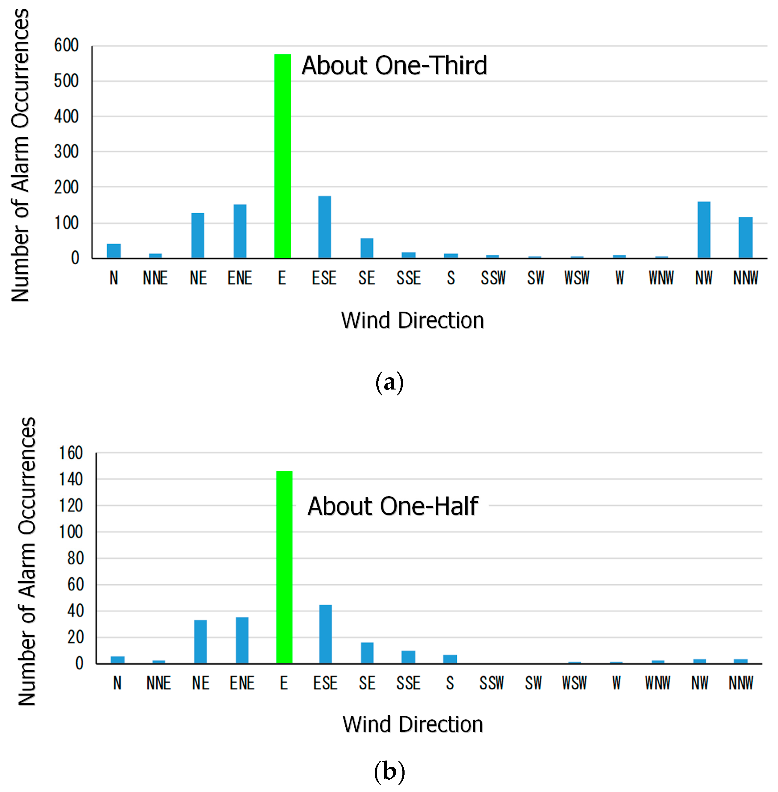
Figure 8.
Result of graphing the values in
Table 3. (
a) Number of alarm occurrences for yaw misalignment. (
b) Number of alarm occurrences for wind direction mismatch of the wind vane. Note: Wind turbine systems resort to shutting down the wind turbine if the yaw misalignment exceeds a threshold.
Figure 8.
Result of graphing the values in
Table 3. (
a) Number of alarm occurrences for yaw misalignment. (
b) Number of alarm occurrences for wind direction mismatch of the wind vane. Note: Wind turbine systems resort to shutting down the wind turbine if the yaw misalignment exceeds a threshold.
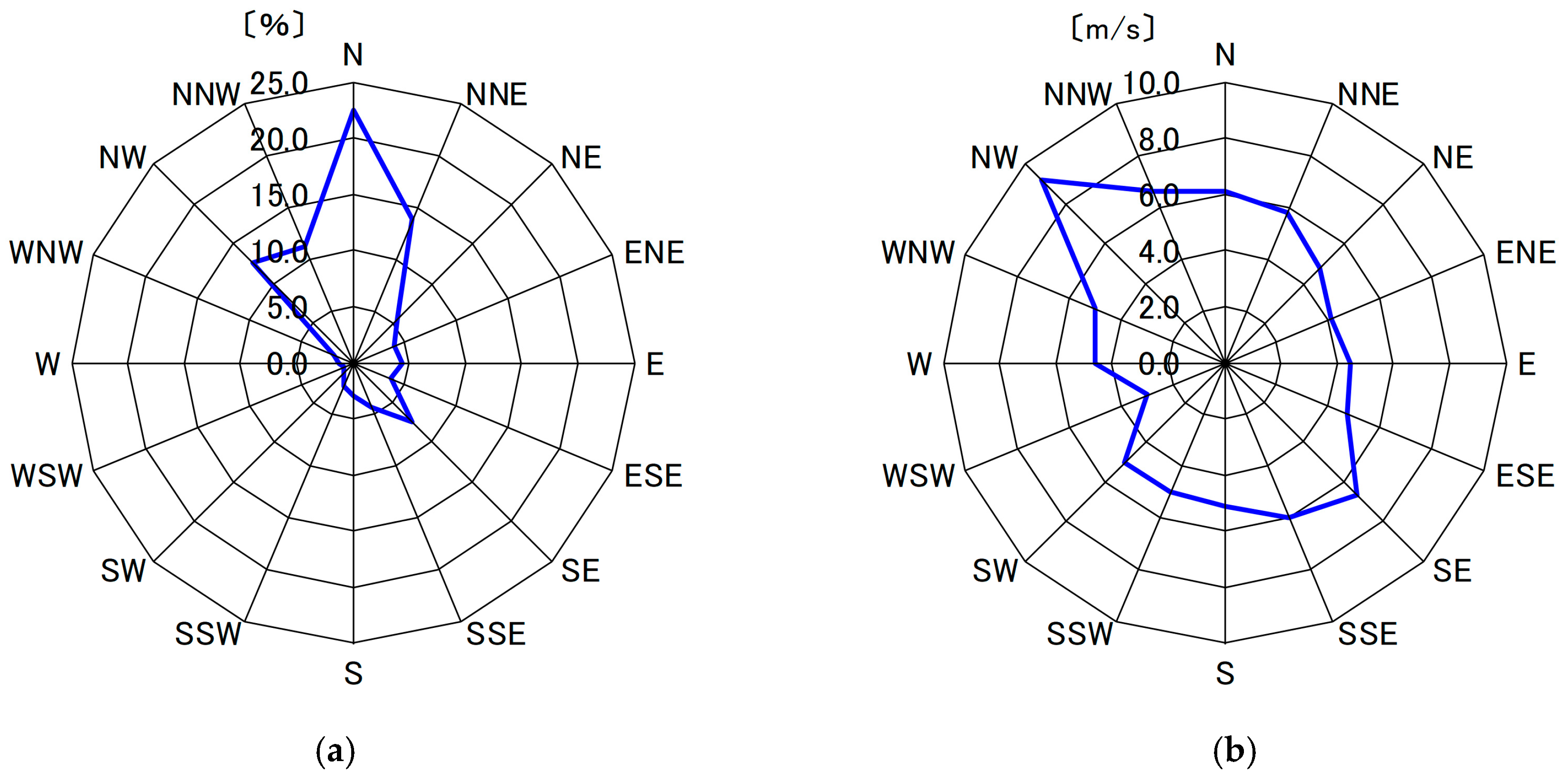
Figure 9.
Frequency distribution of the direction of the 10-min average wind (%): (a) wind rose (frequency distribution) and the average of the 10-min average wind speed observed for 16 wind directions (m/s): (b) wind speed by direction (wind measurement height: hub height (60 m), analysis period: 3 November 2015, 0:00 a.m. JST–17 March 2016, 7:00 a.m. JST).
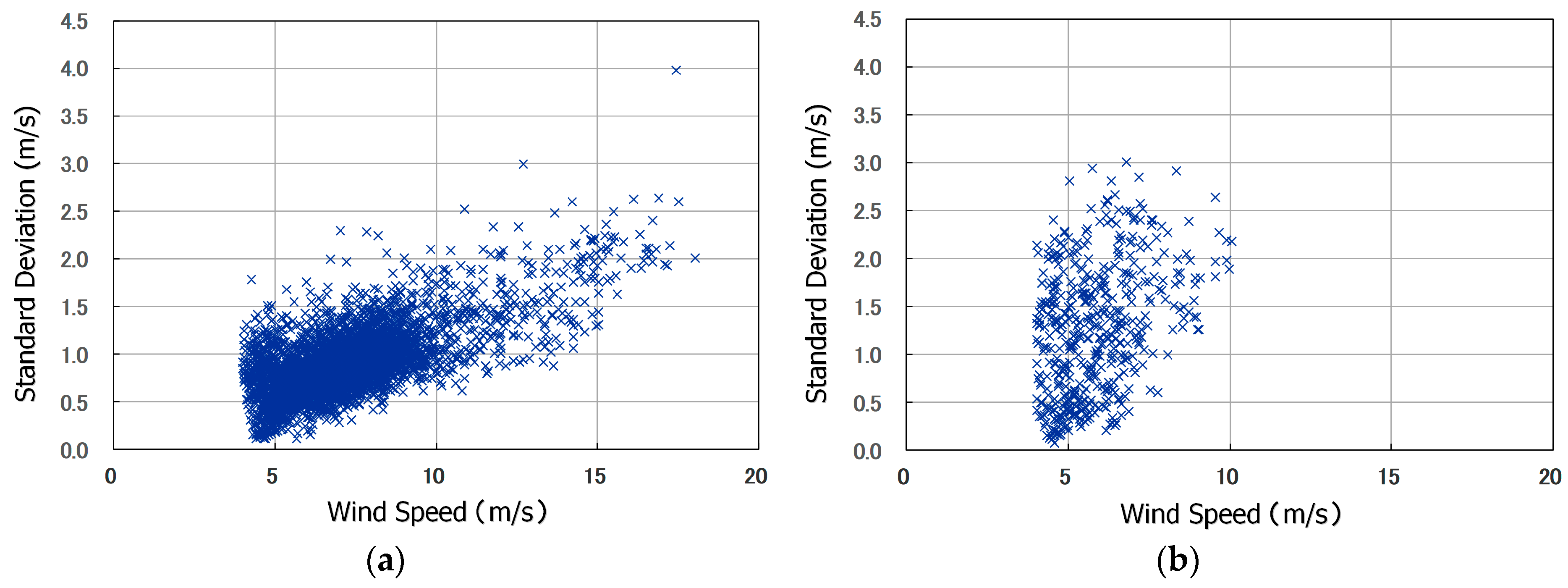
Figure 10.
Relationship between the standard deviation and the average of the wind speed in 10-min periods for two wind directions (wind measurement height: hub-height (60 m), analysis period: 3 November 2015, 0:00 a.m. JST–17 March 2016, 7:00 a.m. JST). (a) Northerly wind. (b) Easterly wind.
Figure 10.
Relationship between the standard deviation and the average of the wind speed in 10-min periods for two wind directions (wind measurement height: hub-height (60 m), analysis period: 3 November 2015, 0:00 a.m. JST–17 March 2016, 7:00 a.m. JST). (a) Northerly wind. (b) Easterly wind.
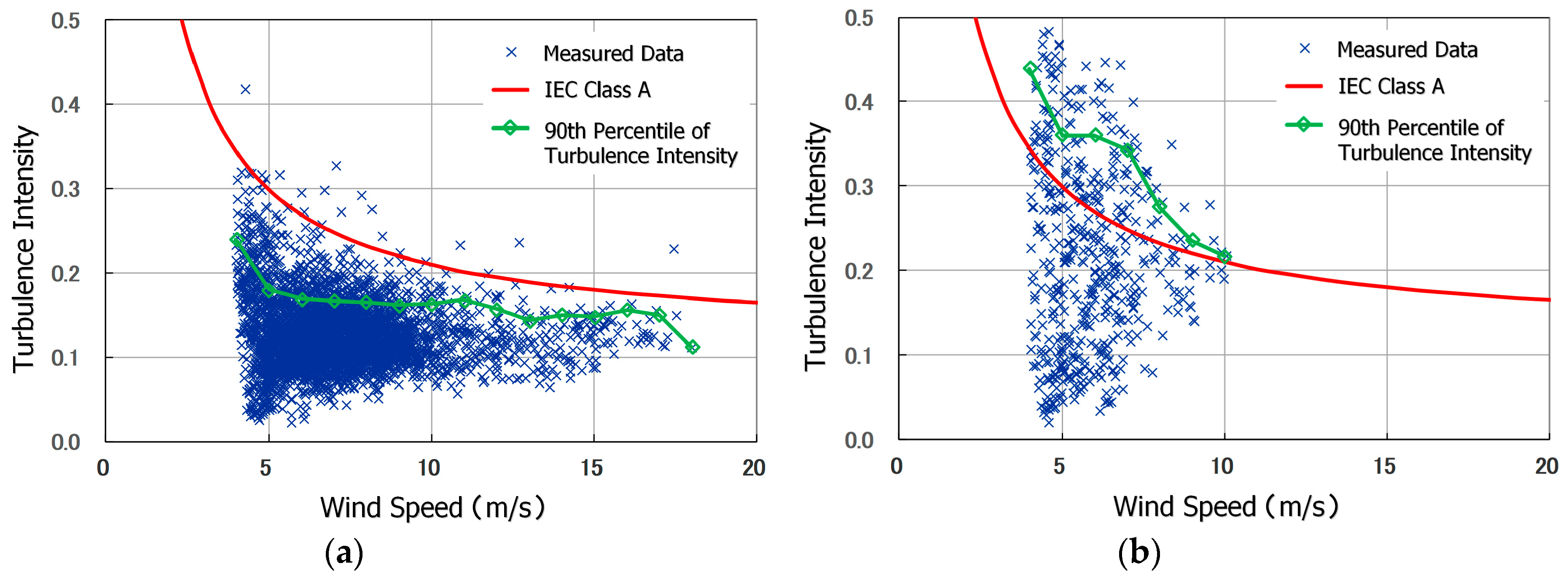
Figure 11.
Relationship between turbulence intensity and the average of the wind speed in 10-min periods for two wind directions (wind measurement height: hub-height (60 m), analysis period: 3 November 2015, 0:00 a.m. JST–17 March 2016, 7:00 a.m. JST). (a) Northerly wind. (b) Easterly wind.
Figure 11.
Relationship between turbulence intensity and the average of the wind speed in 10-min periods for two wind directions (wind measurement height: hub-height (60 m), analysis period: 3 November 2015, 0:00 a.m. JST–17 March 2016, 7:00 a.m. JST). (a) Northerly wind. (b) Easterly wind.
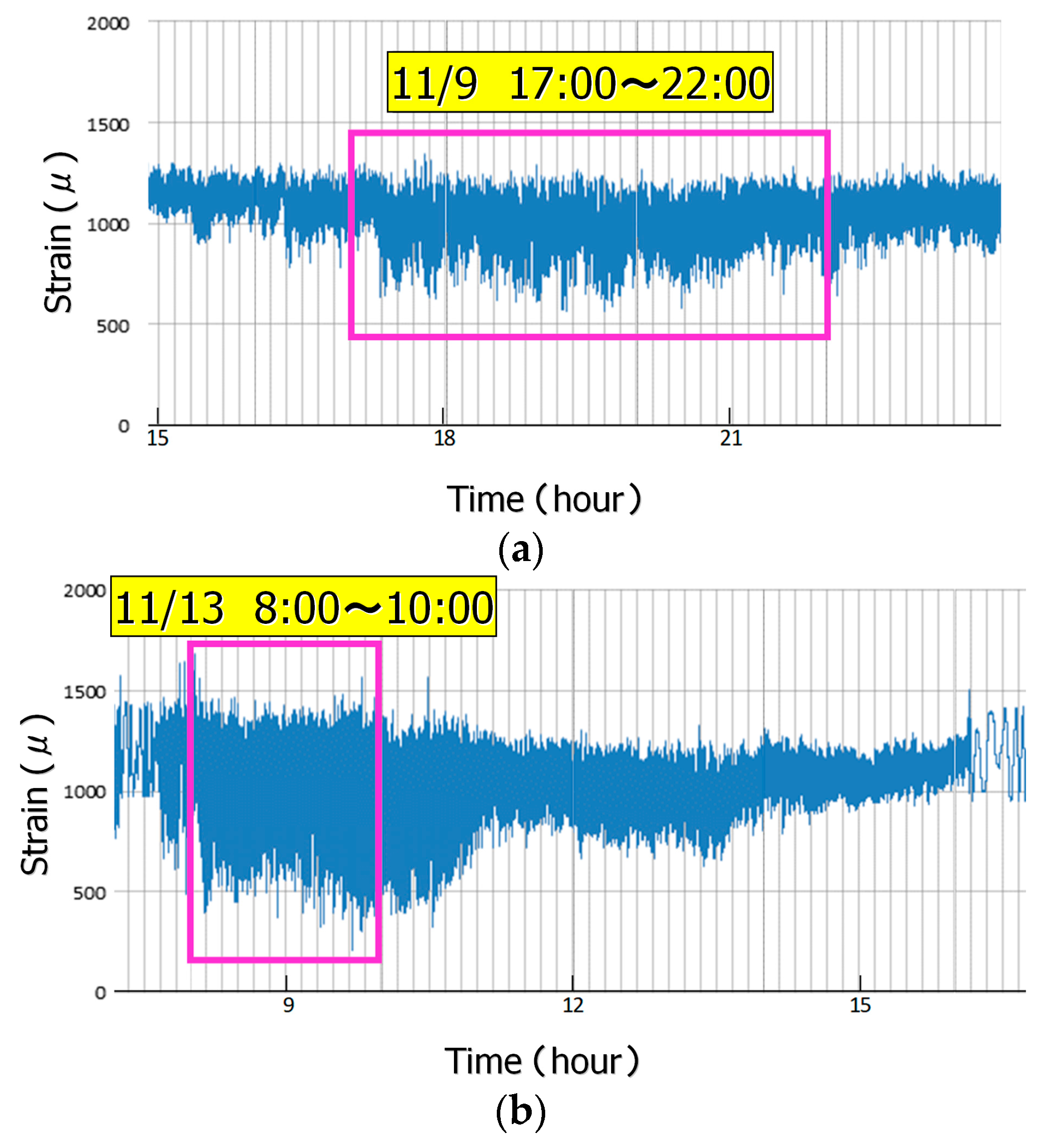
Figure 12.
Blade strain data (blade flapwise bending raw data). (a) Northerly wind. (b) Easterly wind. Note: interval: 0.02 seconds, average wind speed: approx. 9 m/s.
Figure 12.
Blade strain data (blade flapwise bending raw data). (a) Northerly wind. (b) Easterly wind. Note: interval: 0.02 seconds, average wind speed: approx. 9 m/s.
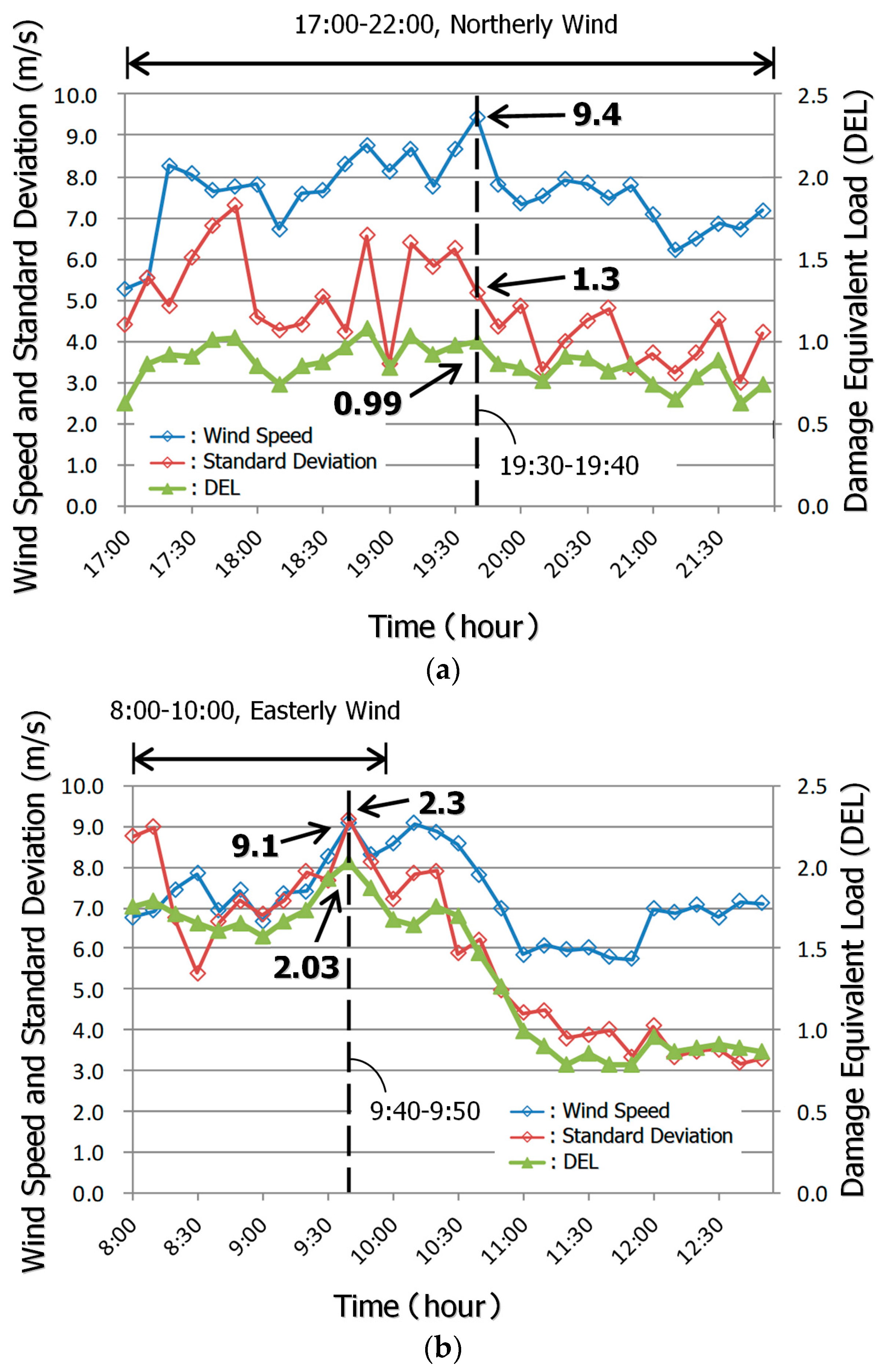
Figure 13.
Time series of wind speed, standard deviation and normalized damage equivalent load (DEL) for flapwise blade bending. Plotted values were evaluated from instantaneous data values within 10-min periods. (a) Northerly wind. (b) Easterly wind.
Figure 13.
Time series of wind speed, standard deviation and normalized damage equivalent load (DEL) for flapwise blade bending. Plotted values were evaluated from instantaneous data values within 10-min periods. (a) Northerly wind. (b) Easterly wind.
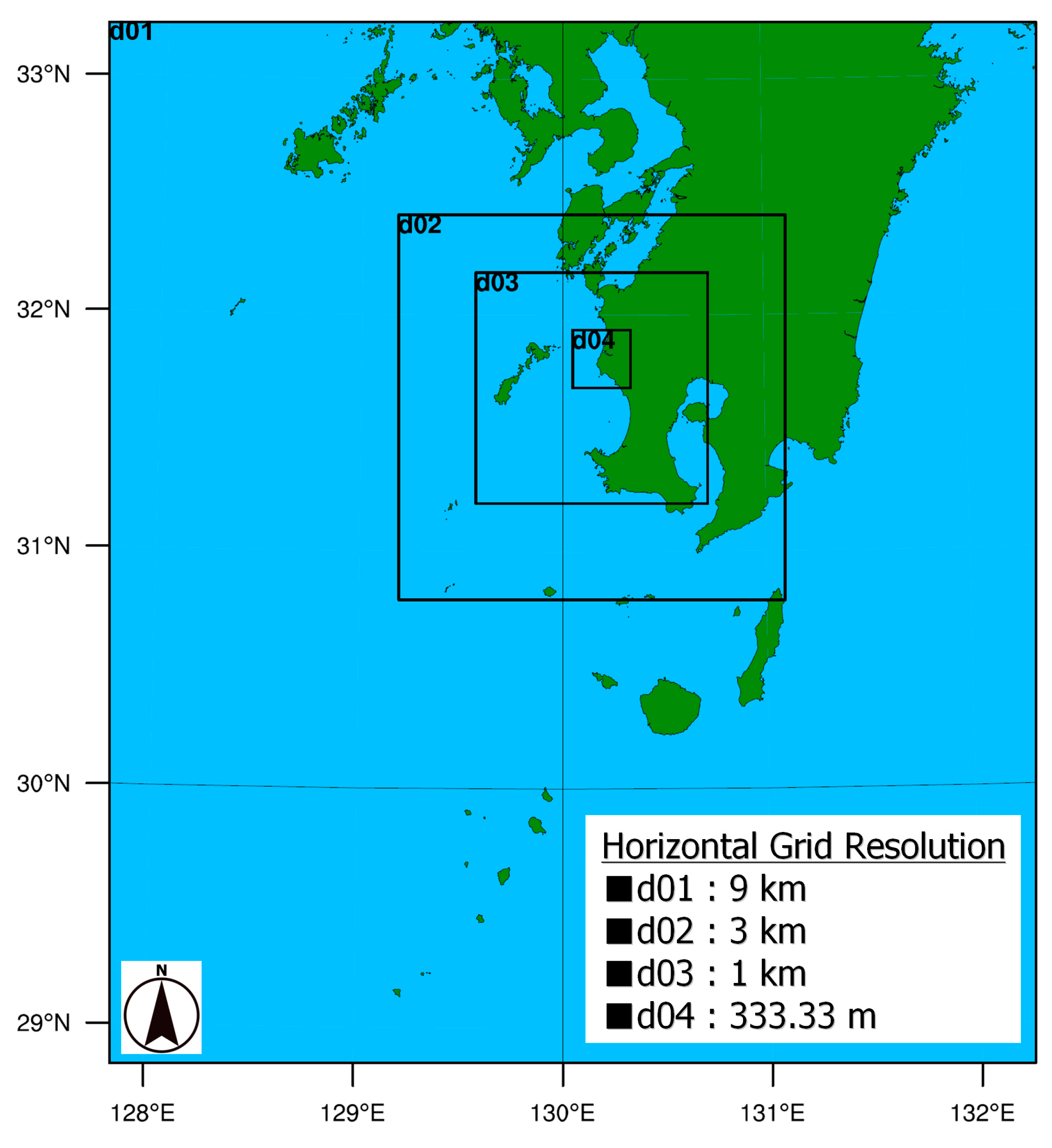
Figure 14.
Computational domain used in the Weather Research and Forecasting (WRF) mesoscale model.
Figure 14.
Computational domain used in the Weather Research and Forecasting (WRF) mesoscale model.
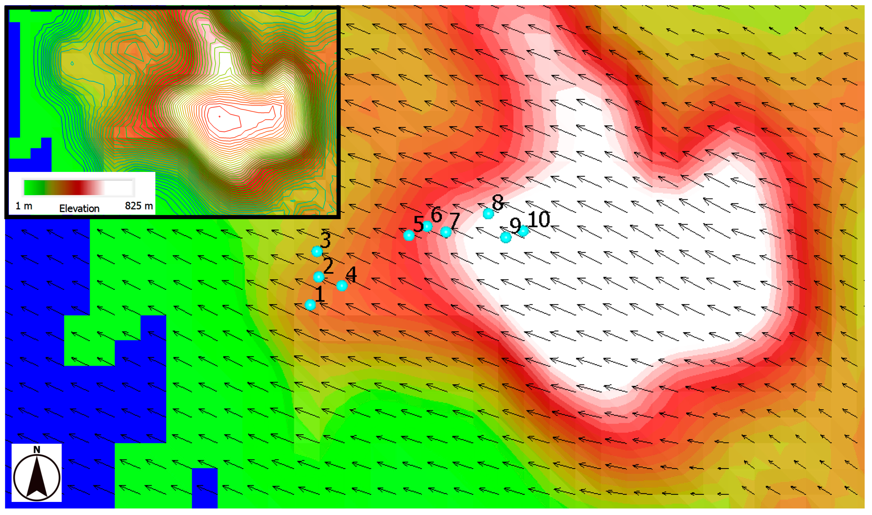
Figure 15.
Distribution of the horizontal wind vectors in Domain 4, approximately 60 m above the ground surface. 9:40 a.m. JST, Nov. 13, 2015.
Figure 15.
Distribution of the horizontal wind vectors in Domain 4, approximately 60 m above the ground surface. 9:40 a.m. JST, Nov. 13, 2015.
Figure 16.
Comparison of the topographic section. (a) Northerly wind. (b) Easterly wind.
Figure 16.
Comparison of the topographic section. (a) Northerly wind. (b) Easterly wind.
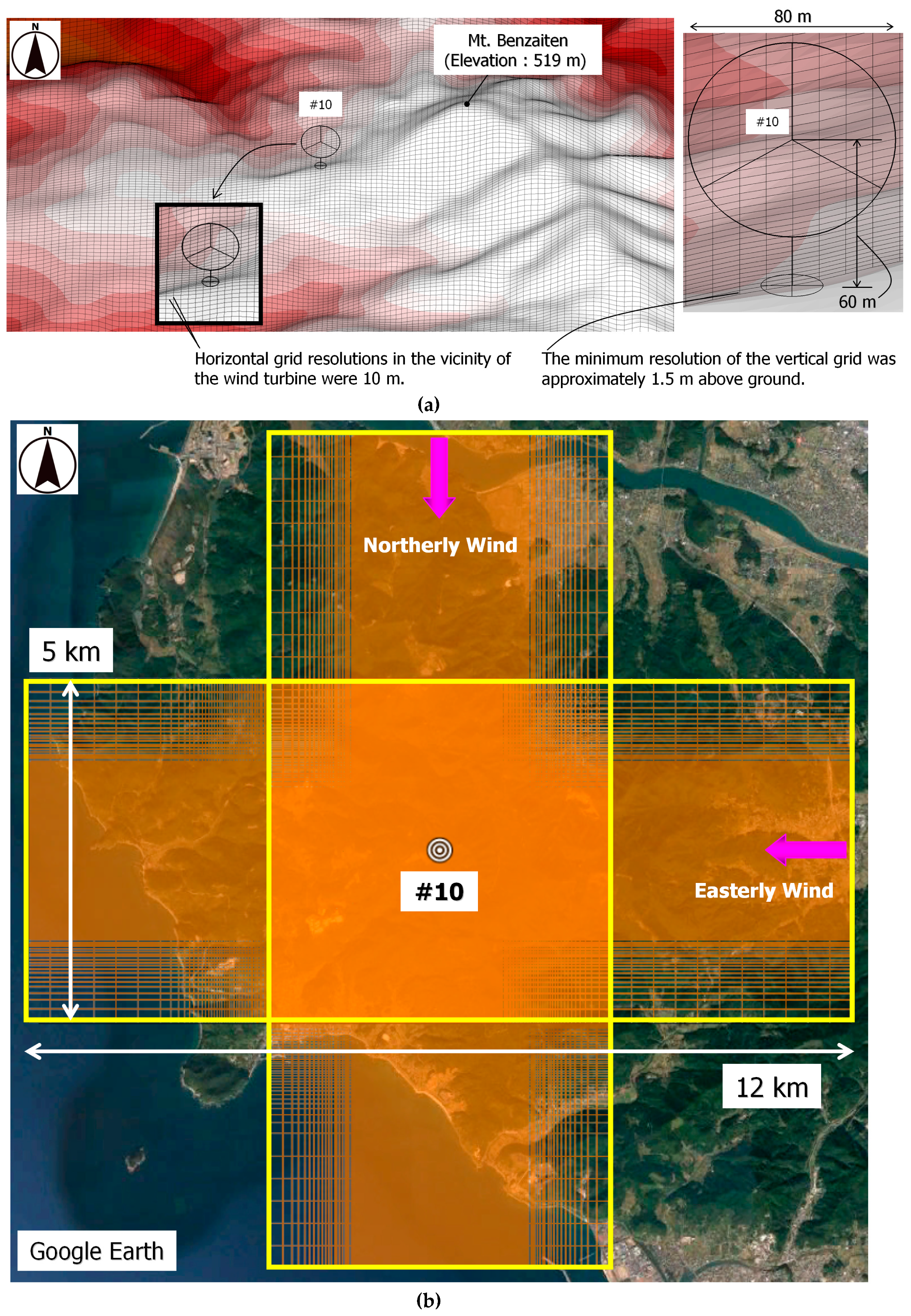
Figure 17.
Computational grids and domain. (a) Enlarged view. (b) Overall view.
Figure 17.
Computational grids and domain. (a) Enlarged view. (b) Overall view.
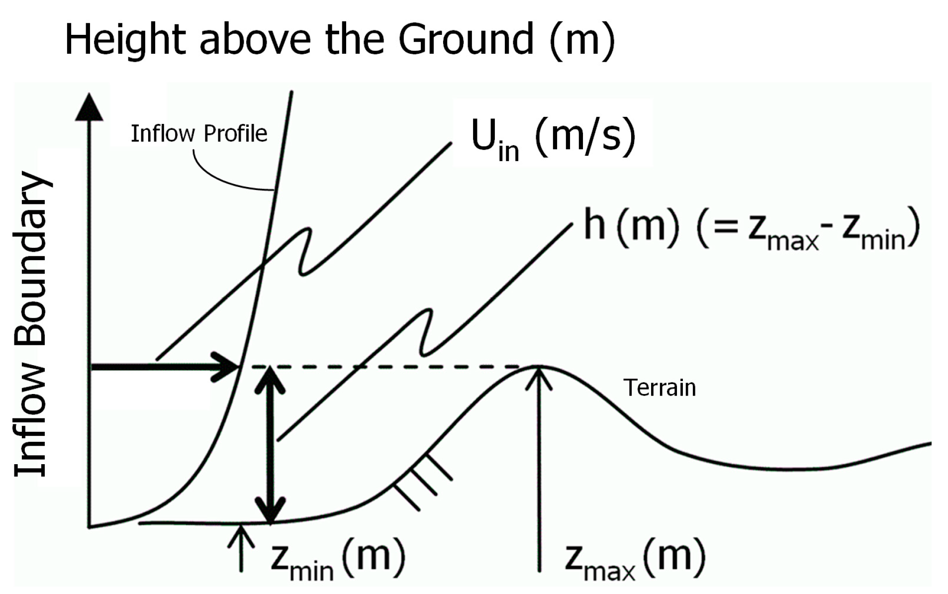
Figure 18.
Inflow condition.
Figure 18.
Inflow condition.
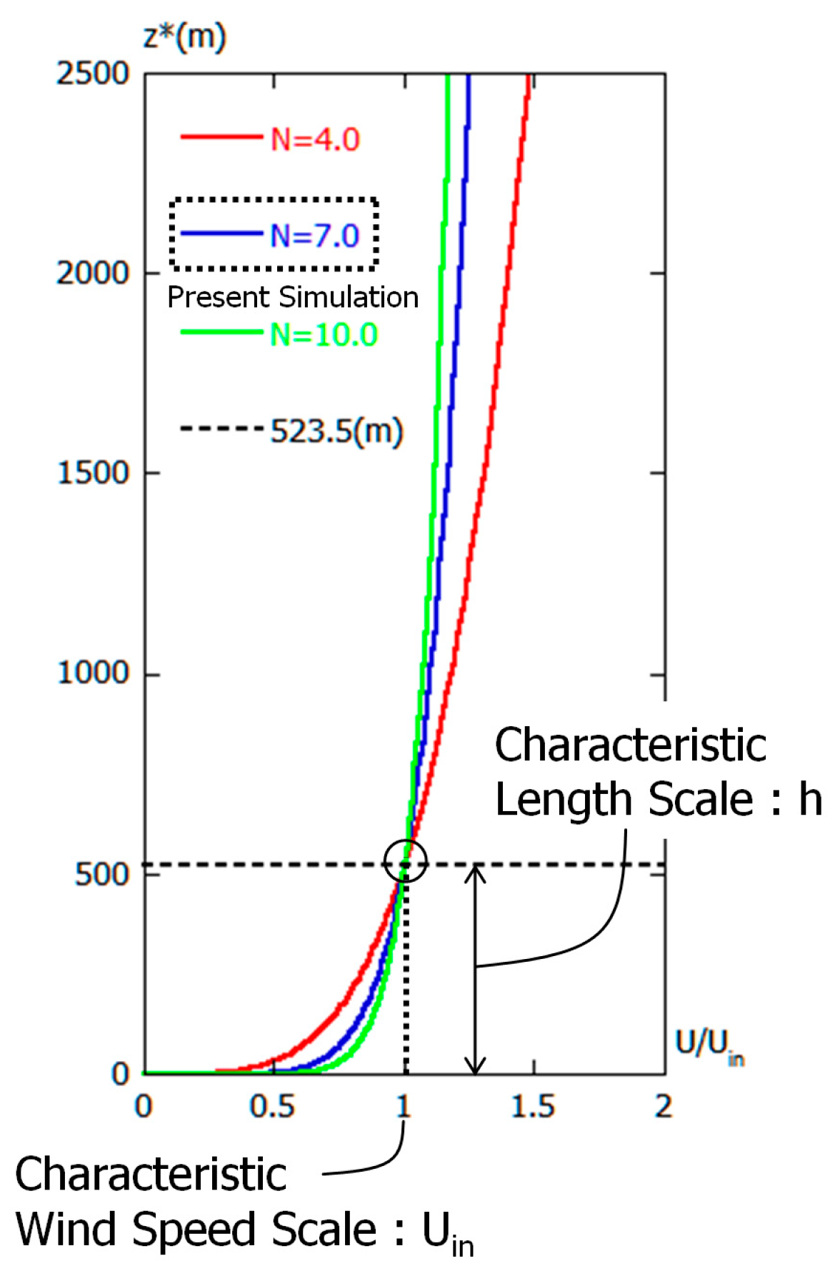
Figure 19.
Two characteristic scales (Uin and h).
Figure 19.
Two characteristic scales (Uin and h).
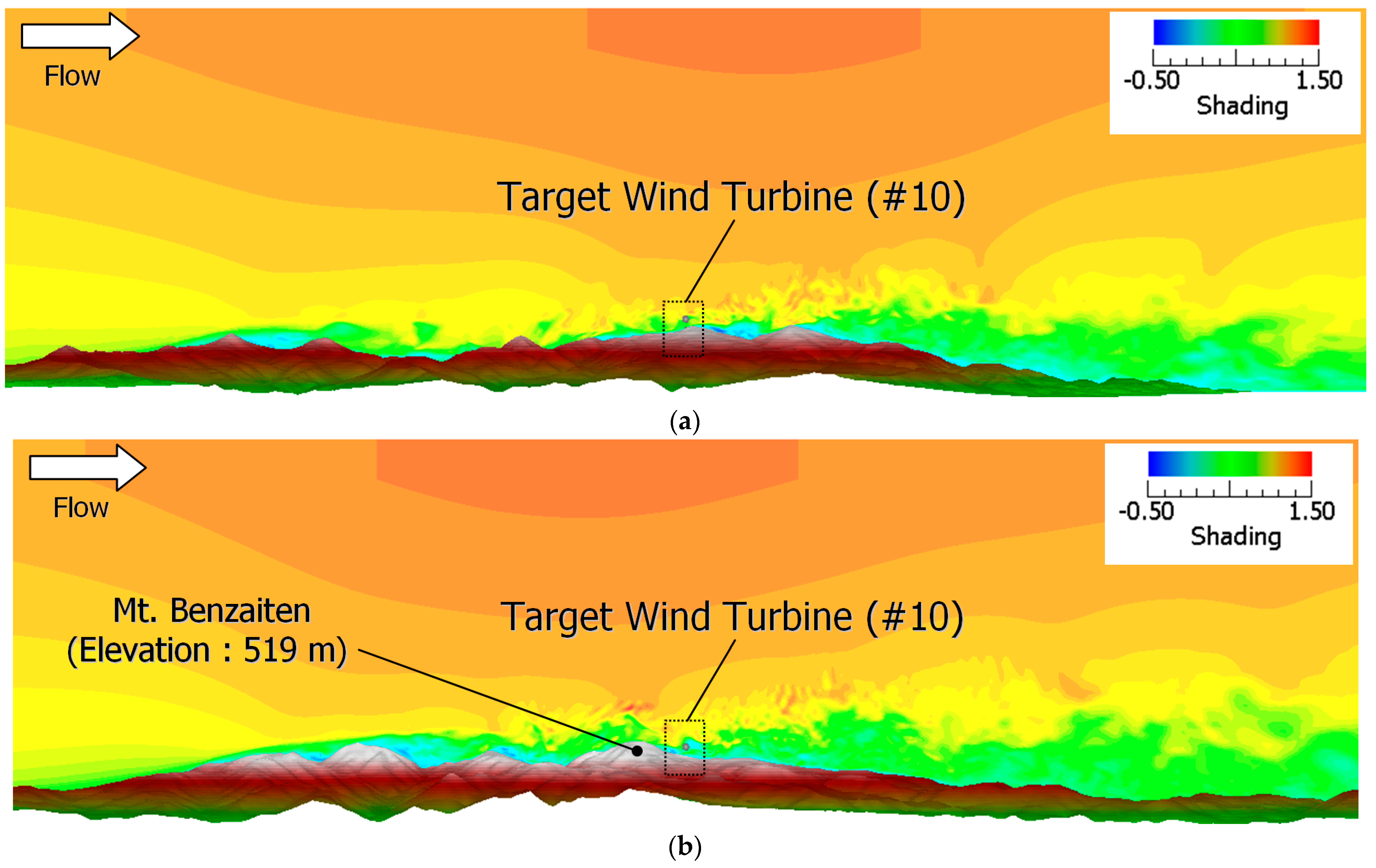
Figure 20.
Distribution of the streamwise wind velocity component on a vertical cross-section that includes wind turbine #10 and the instantaneous flow field. (a) Northerly wind. (b) Easterly wind.
Figure 20.
Distribution of the streamwise wind velocity component on a vertical cross-section that includes wind turbine #10 and the instantaneous flow field. (a) Northerly wind. (b) Easterly wind.
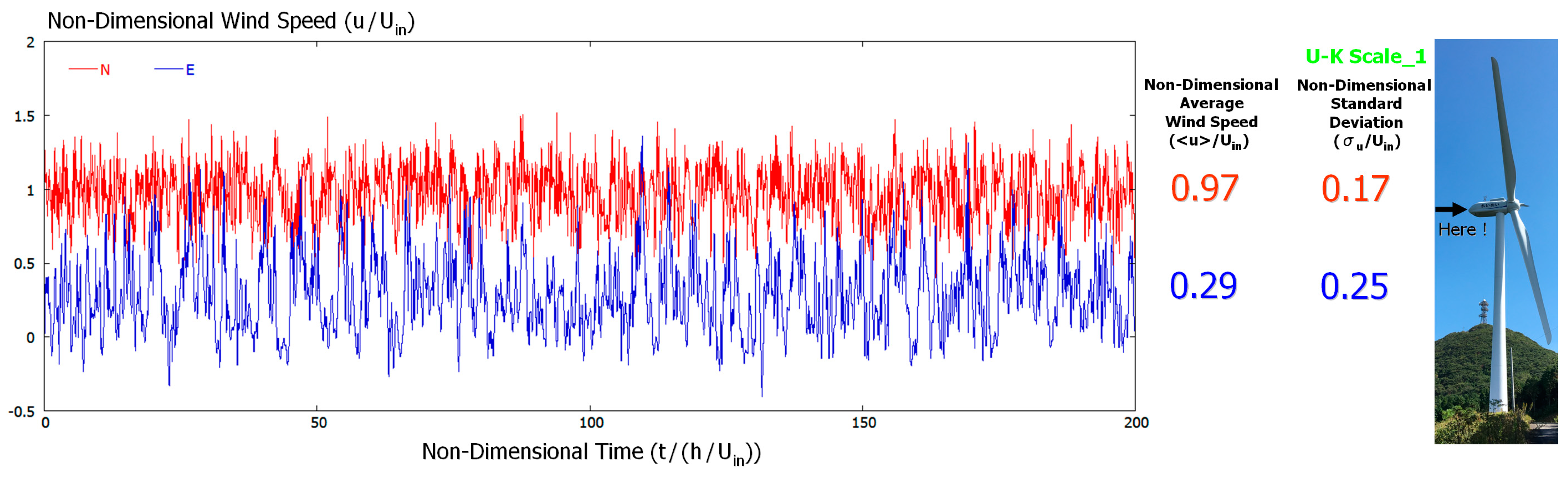
Figure 21.
Time-series data of streamwise wind velocity from the numerical simulations. Red: northerly wind, Blue: easterly wind.
Figure 21.
Time-series data of streamwise wind velocity from the numerical simulations. Red: northerly wind, Blue: easterly wind.
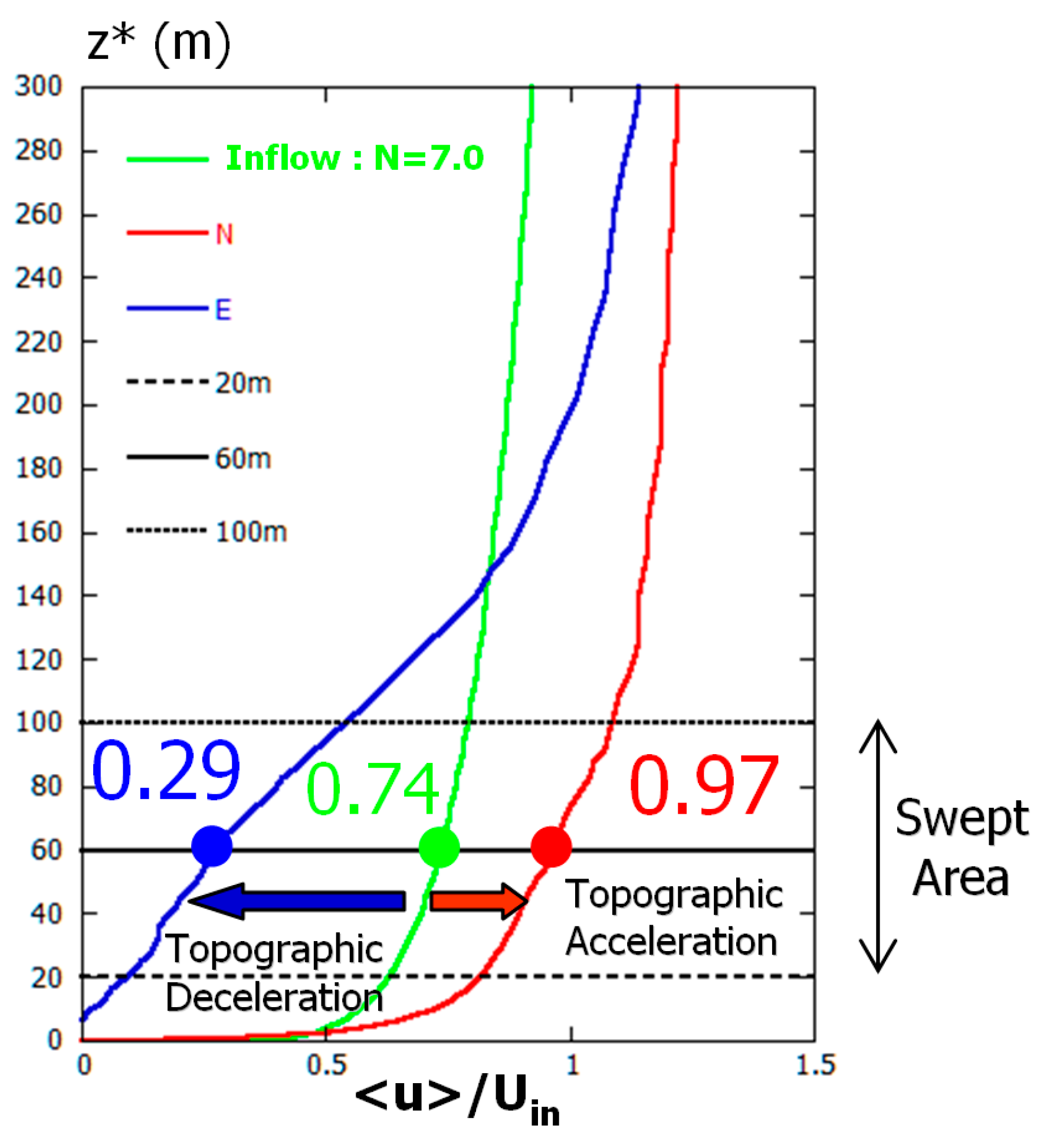
Figure 22.
Vertical profiles of the streamwise wind velocity at wind turbine #10, with a time-averaged flow field. Red: northerly wind, Blue: easterly wind.
Figure 22.
Vertical profiles of the streamwise wind velocity at wind turbine #10, with a time-averaged flow field. Red: northerly wind, Blue: easterly wind.
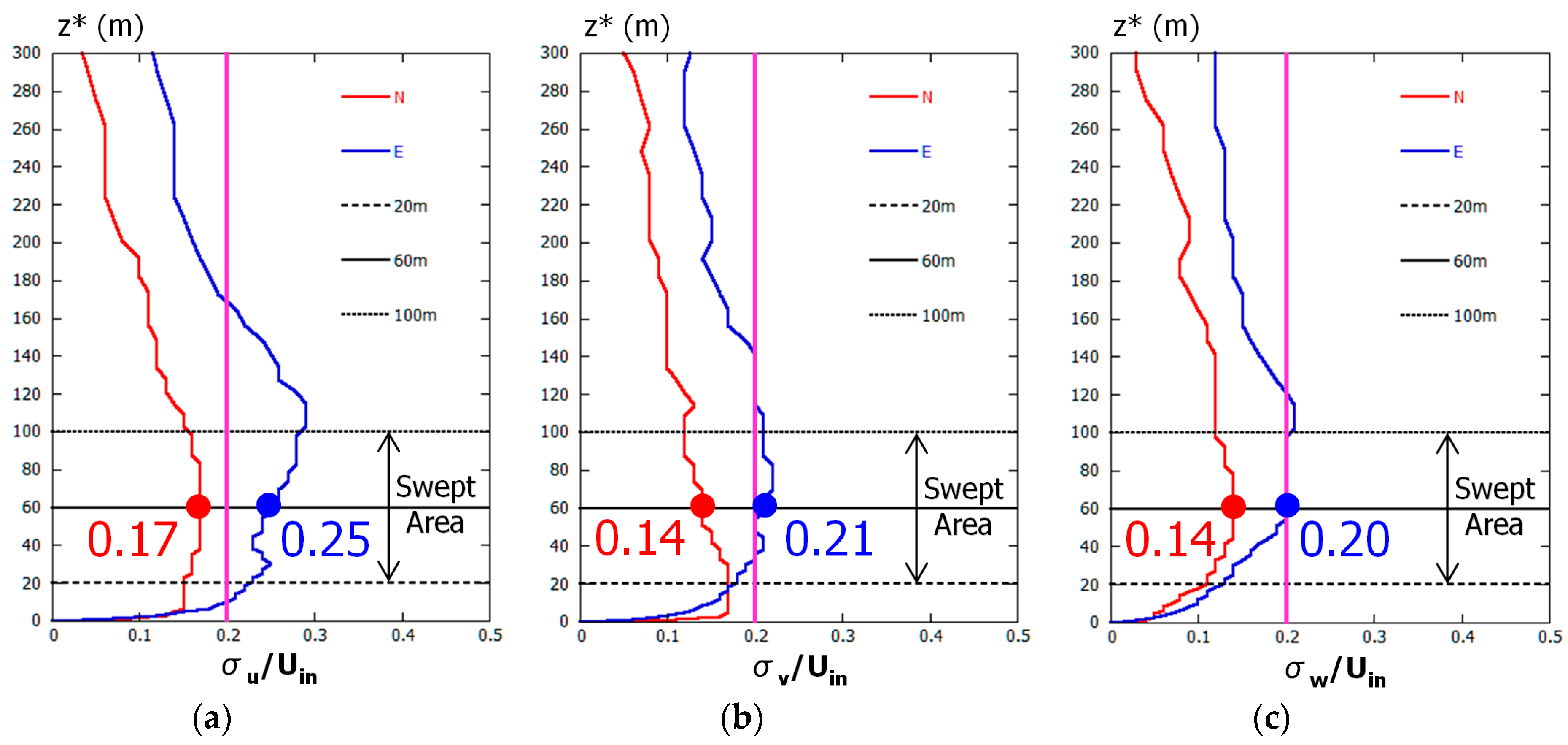
Figure 23.
Vertical profiles of the non-dimensional standard deviations at wind turbine #10, with a time-averaged flow field. Red: northerly wind, Blue: easterly wind. (a) Streamwise direction. (b) Spanwise direction. (c) Vertical direction.
Figure 23.
Vertical profiles of the non-dimensional standard deviations at wind turbine #10, with a time-averaged flow field. Red: northerly wind, Blue: easterly wind. (a) Streamwise direction. (b) Spanwise direction. (c) Vertical direction.
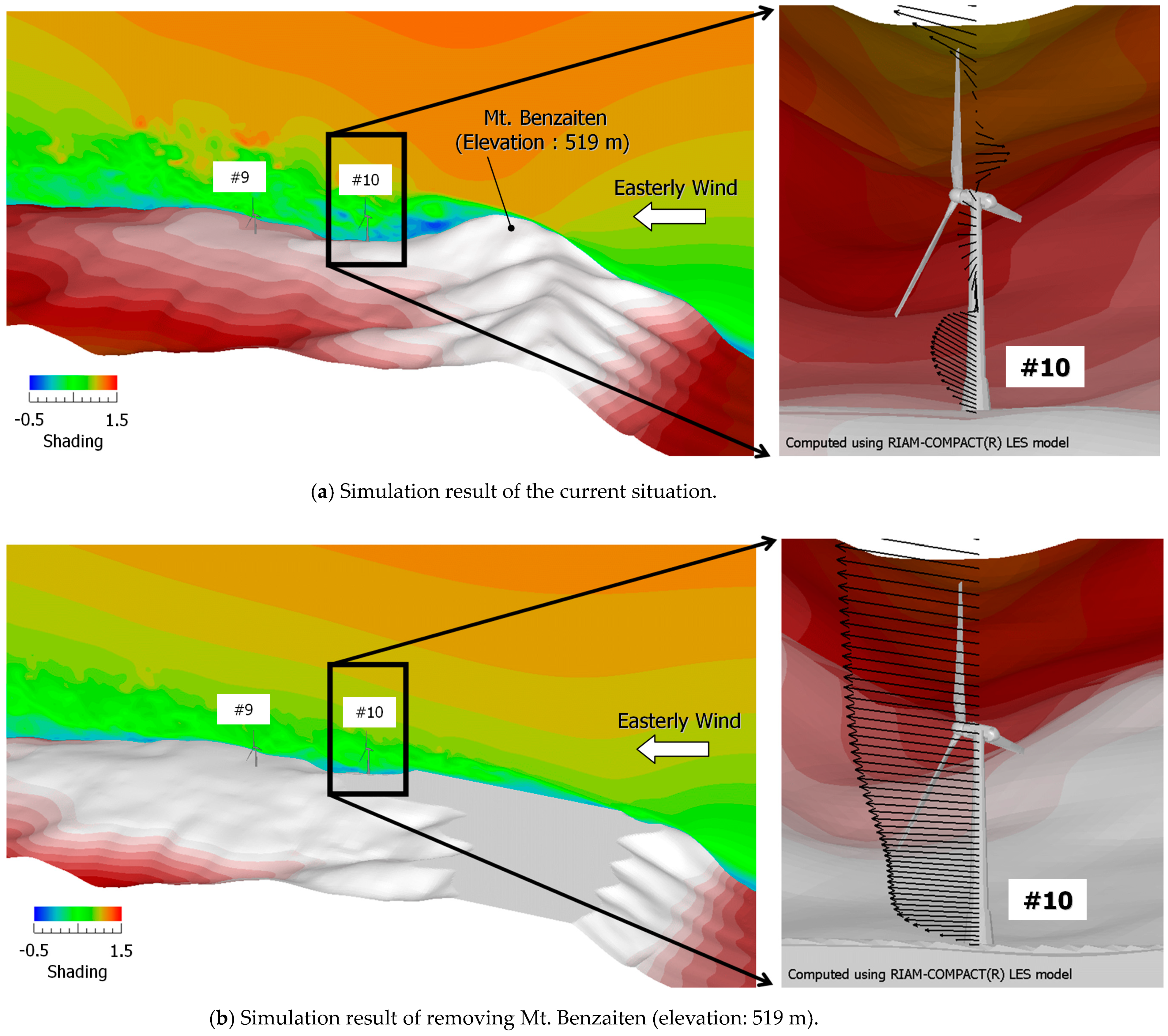
Figure 24.
Distribution of the streamwise wind velocity component on a vertical cross-section, which includes wind turbine #10 and wind velocity vectors at wind turbine #10, easterly wind, and instantaneous flow field.
Figure 24.
Distribution of the streamwise wind velocity component on a vertical cross-section, which includes wind turbine #10 and wind velocity vectors at wind turbine #10, easterly wind, and instantaneous flow field.
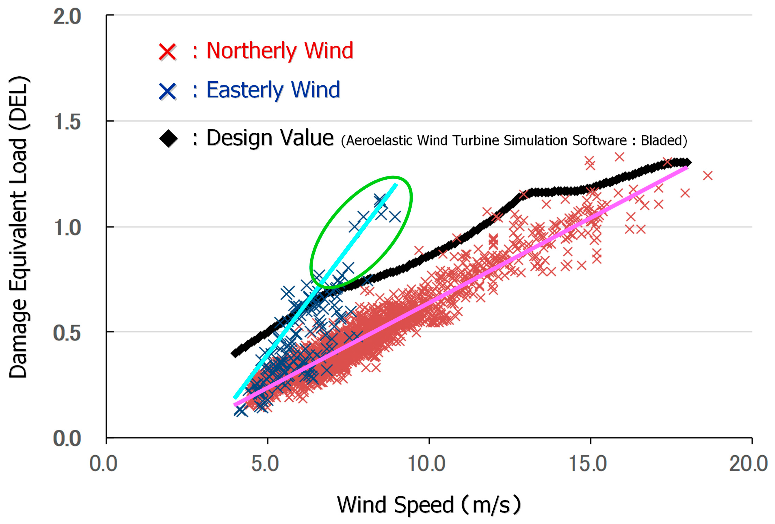
Figure 25.
Relationship between wind speed (m/s) and damage equivalent load (DEL).
Figure 25.
Relationship between wind speed (m/s) and damage equivalent load (DEL).
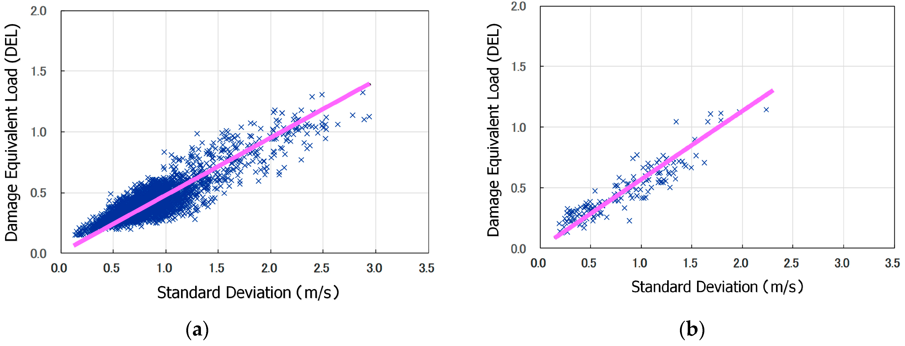
Figure 26.
Relationship between standard deviation (m/s) and damage equivalent load (DEL). (a) Northerly wind. (b) Easterly wind.
Figure 26.
Relationship between standard deviation (m/s) and damage equivalent load (DEL). (a) Northerly wind. (b) Easterly wind.
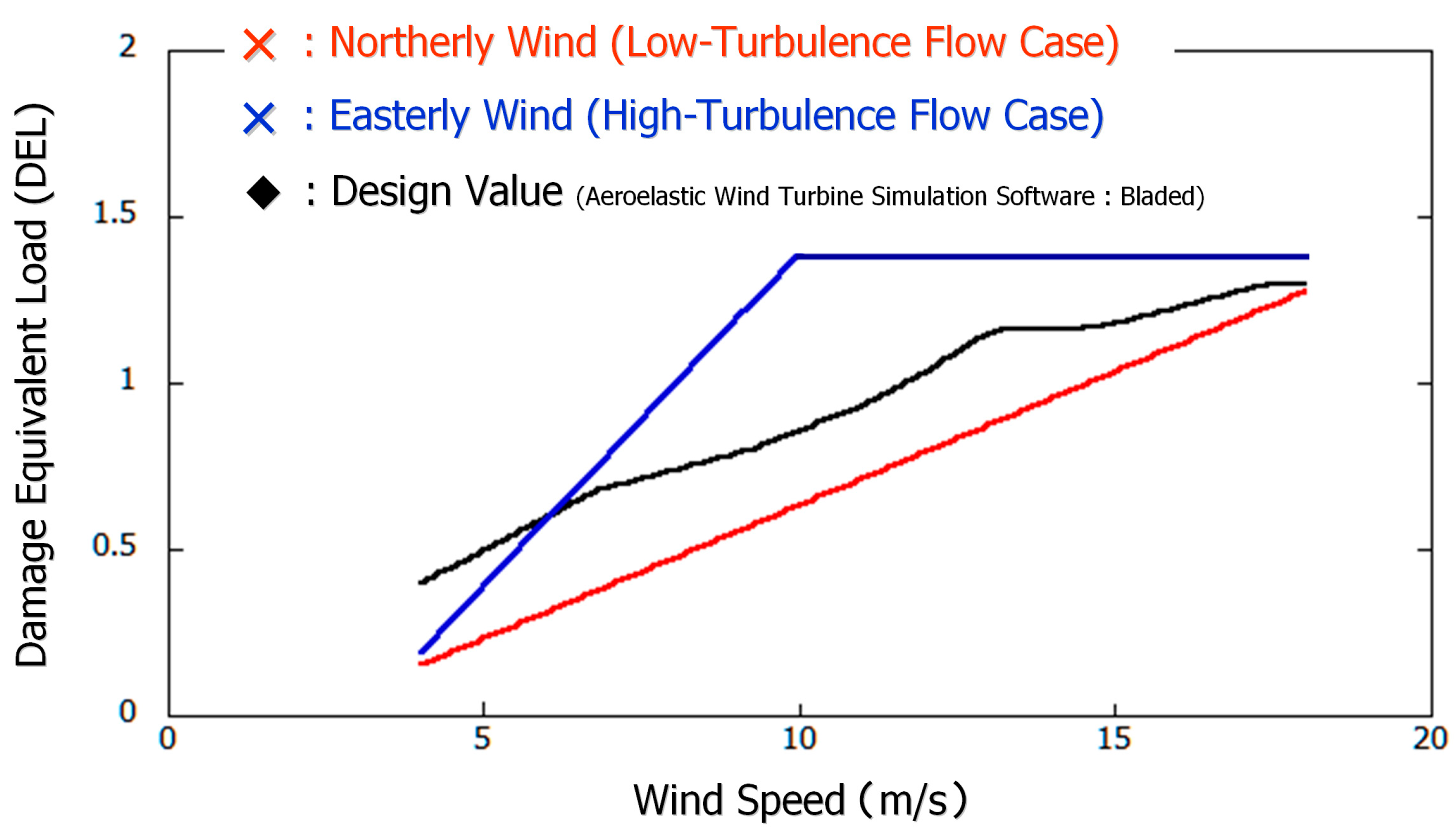
Figure 27.
Regression line between wind speed (m/s) and damage equivalent load (DEL).
Figure 27.
Regression line between wind speed (m/s) and damage equivalent load (DEL).
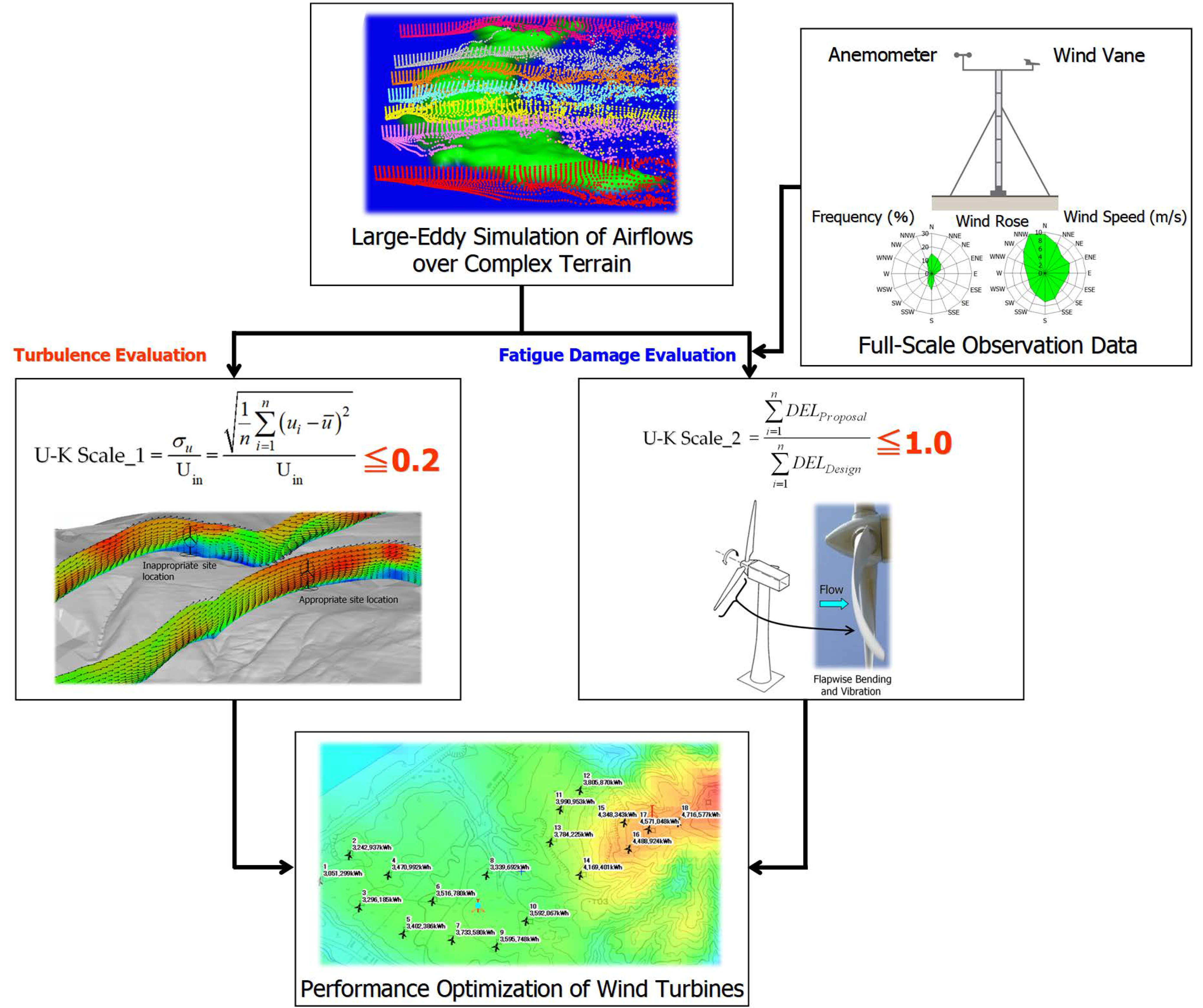
Figure 28.
An example of wind energy resource assessment based on the two reference scales (the U-K scales).
Figure 28.
An example of wind energy resource assessment based on the two reference scales (the U-K scales).
Table 1.
Elevation information for wind turbine #10 and distance between Mt. Benzaiten (elevation 519 m) and wind turbine #10.
Table 1.
Elevation information for wind turbine #10 and distance between Mt. Benzaiten (elevation 519 m) and wind turbine #10.
| Elevation at Base of Wind Turbine #10 | Maximum Blade Tip Elevation (Above Sea Level) | Distance Between Mt. Benzaiten and Wind Turbine #10 |
|---|
| 418 m | 518 m | Approx. 300 m |
Table 2.
Number of alarm occurrences for wind conditions under all wind directions.
Table 2.
Number of alarm occurrences for wind conditions under all wind directions.
| Alarm Item | Wind Turbine #10 | Other Wind Turbines (Average) |
|---|
| Shutdown due to excessive yaw error | 1448 | 530 |
| Discordance in wind directions of sensors | 308 | 80 |
Table 3.
Number of alarm occurrences due to wind conditions for each wind direction.
Table 3.
Number of alarm occurrences due to wind conditions for each wind direction.
| Alarm Item | N | NNE | NE | ENE | E | ESE | SE | SSE | |
| Shutdown due to excessive yaw error | 39 | 12 | 130 | 150 | 560 | 176 | 58 | 18 | |
| Discordance in wind directions of sensors | 5 | 2 | 33 | 35 | 146 | 45 | 16 | 10 | |
| Alarm Item | S | SSW | SW | WSW | W | WNW | NW | NNW | Total |
| Shutdown due to excessive yaw error | 11 | 7 | 2 | 2 | 8 | 2 | 158 | 115 | 1448 |
| Discordance in wind directions of sensors | 6 | 0 | 0 | 1 | 1 | 2 | 3 | 3 | 308 |
Table 4.
Frequency distribution of the direction of the 10-min average wind (%) and the average of the 10-min average wind speed observed for 16 directions (wind measurement height: hub height (60 m), analysis period: 3 November 2015, 0:00 a.m. JST–17 March 2016, 7:00 a.m. JST).
Table 4.
Frequency distribution of the direction of the 10-min average wind (%) and the average of the 10-min average wind speed observed for 16 directions (wind measurement height: hub height (60 m), analysis period: 3 November 2015, 0:00 a.m. JST–17 March 2016, 7:00 a.m. JST).
| Height | Item | N | NNE | NE | ENE | E | ESE | SE | SSE | S | SSW | SW | WSW | W | WNW | NW | NNW | Total |
|---|
| 60 m | Frequency Distribution (%) | 22.5 | 13.8 | 5.6 | 4.0 | 4.4 | 3.6 | 7.5 | 4.3 | 3.0 | 2.2 | 1.2 | 0.9 | 1.3 | 1.8 | 12.6 | 11.2 | 100.0 |
| Average Wind Speed (m/s) | 6.1 | 5.8 | 4.8 | 4.1 | 4.5 | 4.7 | 6.7 | 6.0 | 5.1 | 5.0 | 5.0 | 3.0 | 4.6 | 5.0 | 9.2 | 6.6 | 6.1 |
Table 5.
Wind direction range and total number of data values.
Table 5.
Wind direction range and total number of data values.
| | Wind Direction Range | Total Number of 10-min Periods for Which Wind Statistics are Calculated |
|---|
| Northerly Wind | 0° ± 15° | 4036 (Total: 12,567; 32.1%) |
| Easterly Wind | 90° ± 15° | 496 (Total: 12,567; 4.0%) |
Table 6.
Comparison of the values of the U-K Scale_1 at wind turbine hub height (z* = 60 m) under different N values.
Table 6.
Comparison of the values of the U-K Scale_1 at wind turbine hub height (z* = 60 m) under different N values.
| | N = 4.0 | N = 7.0 | N = 10.0 | Criteria of the U-K Scale_1 |
|---|
| Northerly Wind | 0.16 | 0.17 | 0.17 | 0.20 |
| Easterly Wind | 0.24 | 0.25 | 0.24 |
Table 7.
Values of the U-K Scale_1 with horizontal grid resolution set to 5 m.
Table 7.
Values of the U-K Scale_1 with horizontal grid resolution set to 5 m.
| | Easterly Wind, N = 7.0 | Criteria of the U-K Scale_1 |
|---|
| Case of Removing Mt. Benzaiten (elevation 519 m) | 0.01 | 0.20 |
| Current Situation | 0.28 |


