A Novel Analytical Modeling of a Loop Heat Pipe Employing the Thin-Film Theory: Part I—Modeling and Simulation

Abstract

In this study, steady-state analytical modeling of a loop heat pipe (LHP) equipped with a flat evaporator is presented to predict the temperatures and pressures at each important part of the LHP—evaporator, liquid reservoir (compensation chamber), vapor-transport tube, liquid-transport tube, and condenser. Additionally, this study primarily focuses on analysis of the evaporator—the only LHP component comprising a capillary structure. The liquid thin-film theory is considered to determine pressure and temperature values concerning the region adjacent to the liquid-vapor interface within the evaporator. The condensation-interface temperature is subsequently evaluated using the modified kinetic theory of gases. The present study introduces a novel method to estimate the liquid temperature at the condensation interface. Existence of relative freedom is assumed with regard to the condenser configuration, which is characterized by a simplified liquid–vapor interface. The results obtained in this study demonstrate the effectiveness of the proposed steady-state analytical model with regard to the effect of design variables on LHP heat-transfer performance. To this end, the condenser length, porosity of its capillary structure, and drop in vapor temperature therein are considered as design variables. Overall, the LHP thermal performance is observed to be reasonably responsive to changes in design parameters.

1. Introduction

A loop heat pipe (LHP) shares with conventional heat pipes fundamental physics including phase change of a working fluid and capillary force. On the other hand, LHPs have unique features, both in the structure and working principle, which distinguish themselves from other types of heat pipes. Typical of these may include the wick confined in the evaporator, inverted meniscus at the liquid-vapor interface, liquid reservoir (compensation chamber) embedded into the evaporator, separation of liquid and vapor lines, etc.

Since the advent of LHPs in the early 1970s, a number of studies were conducted with regard to their operational characteristics and viability for use in engineering applications. LHP-based systems are now being employed in diverse applications, besides those concerning space vehicles, which constituted their primary field of use until recently. They have been used for cooling of high-power electrical and electronic components and solar photovoltaic cooling to enhance the efficiency of renewable energy generation. In addition, quite a few investigations were conducted pertaining to the use of LHPs as heat-transfer devices in solar-photovoltaic systems and water-heating systems [1,2,3,4,5,6], solar-power towers [7,8] and in HVAC systems [9,10,11] to enhance the heat transfer performance. Specific information and discussions regarding the use of LHPs can be found in [12,13]. Most initially developed LHP configurations employed ammonia as the working fluid enclosed within a cylindrical evaporator. Recently, flat or disk-shaped evaporator structures have also been considered owing to their ease of use as heat sources and excellent thermal-contact performance. Additionally, investigations have been performed to identify alternate capillary geometries and working fluids suitable for use in commercial applications.

Physical considerations have typically assumed great importance during theoretical analysis of LHPs and associated thermal performance prediction. Several studies [13,14,15] have reported mathematical modeling of the physical behavior of working fluids at certain locations within the evaporator. Khrustalev and Faghri [13] employed the thin-film theory to analyze the configuration of and interface temperature across the gas–liquid interface (meniscus) in the evaporator as it recedes towards the interior of the capillary structure in the event of a dry-out. Yu et al. [5], Zhao and Liao [14], and Kaya and Goldak [15] performed studies focusing on the thermal-hydraulic analysis of LHP capillary structures, thereby providing appropriate mathematical descriptions for several types of operating limits, such as the critical LHP heat flux, overheating limit, and boiling limit. Chernysheva et al. [16] performed heat-transfer analysis of an LHP compensation chamber to demonstrate the effect of a bayonet on the system’s heat-transfer performance. Chernysheva and Maydanik [17] proposed an analytical model for realizing heat and mass transfers radially within a cylindrical evaporator, and calculation results obtained using the said model demonstrated existence of a radial pressure drop. Additionally, investigations have recently been performed concerning heat leakage from the capillary structure to the compensation chamber [18,19] along with development of a mathematical model [20] that quantifies the effect of cylindrical-evaporator length on thermal performance. Such models have demonstrated great utility in shedding light on the internal physical behavior of LHPs; however, they do not comprehensively describe the heat-transfer performance of the entire system. Individual models for predicting the steady-state performance of LHP components—evaporator, vapor line, condenser, and liquid line—have previously been proposed by Furukawa [21], Abhijit et al. [22], Launay et al. [23], and Bai et al. [24]. These models, in combination, facilitate prediction of the effect of LHP-system design variables on heat-transfer performance. The utility of these models is, however, limited in that they do not account for energy conservation within the liquid reservoir by combining thermal energies associated with the condenser and the said reservoir. Consequently, the condenser-outlet temperature obtained based on the geometrical size and cooling conditions concerning the condenser does not affect evaporator temperature distributions. Additionally, Pouzet et al. [25], Vlassov and Riehl [26], and Kaya et al. [27] have proposed transient LHP-analysis models. However, a detailed model capable of reliably predicting the overall operating characteristics of an LHP system is yet to be developed and/or demonstrated.

The present study describes development of a steady-state analysis model concerning operation of the entire LHP system via application of the liquid thin-film theory to the liquid–vapor interface within the capillary structure comprising fine pores. The novelty of this study is described in the following. In the proposed model, the nodal approach technique [28] is employed to estimate the temperature of typical points in the evaporator, whereas the thin-film theory is used to predict the shape of the vapor–liquid interface created within fine pores. The interface temperature is expressed using the kinetic theory of gases [29,30]. A novel method is employed to deduce equations for determining temperatures at which phase change of the working fluid occurs across interfaces as well as the corresponding interface location. Another novelty of this study exists in the way the condenser is treated to determine the temperatures at the condenser outlet and liquid reservoir. The condenser-outlet temperature is predicted using the effectiveness(ε)-NTU method [31], which are commonly employed for analysis and performance simulation of heat exchangers. Furthermore, energy conservation between the condenser outlet and liquid reservoir is considered to determine the liquid-reservoir temperature whilst also demonstrating the impact of condenser-outlet temperature on the liquid reservoir. Lastly, our proposed study comprises two parts. Part I presents development of the steady-state-analysis model of the LHP and associated effects of design variables on the overall heat-transfer performance. Part II, on the other hand, discusses experimental verification of the proposed steady-state analysis model.

2. Mathematical Model for Steady-State Analysis

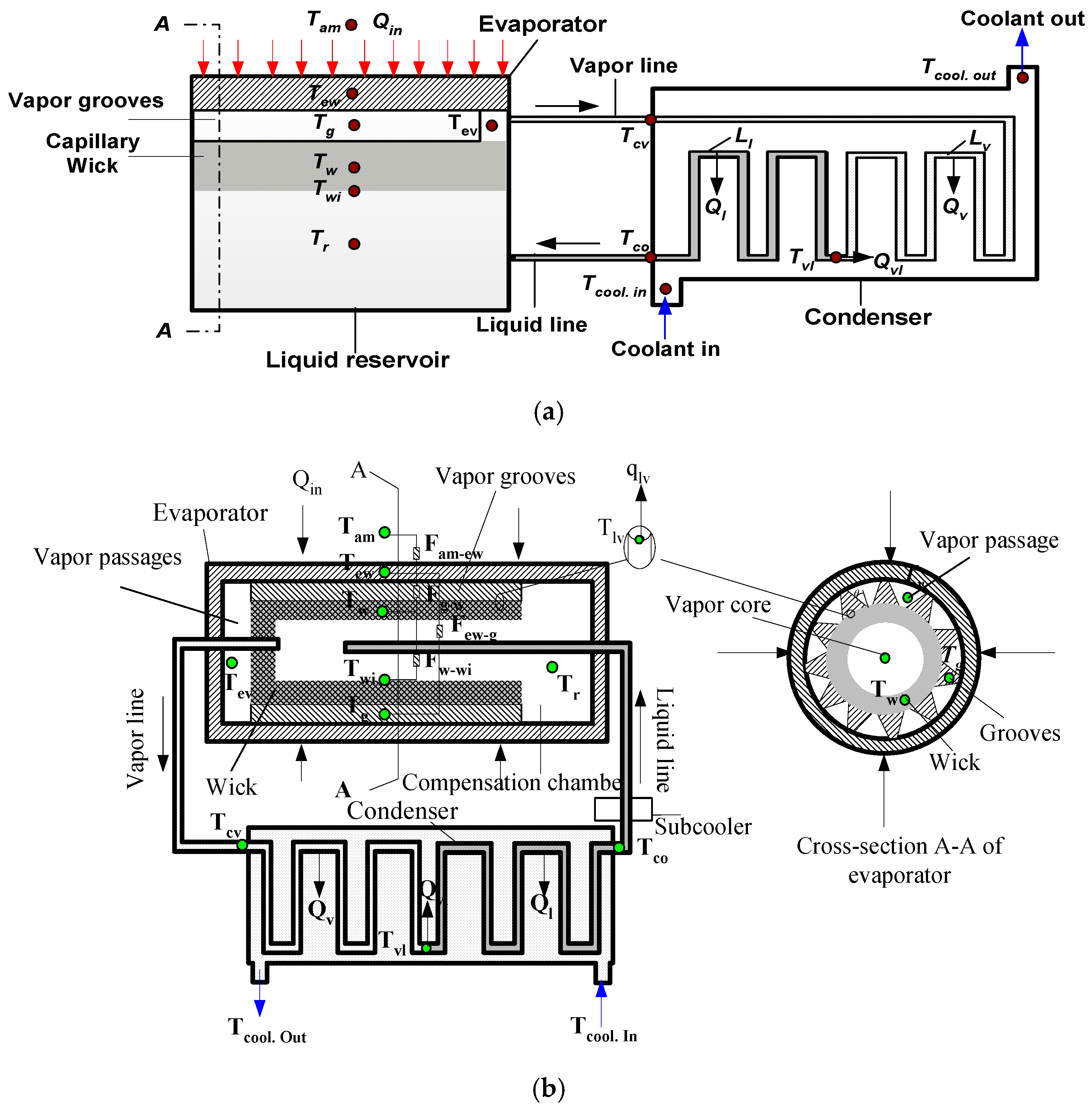
The mathematical model proposed in this study was developed for two LHP types—one with a flat evaporator (FLHP) and another with a cylindrical (CLHP) evaporator, as depicted in Figure 1. The major assumptions made during development of the proposed model are:

• Evaporation only occurs on the contact surface between the capillary structure and grooves (i.e., vapor removal flow path within LHP); additionally, two-phase flows are not considered herein in favor of exclusive pure vapor and liquid flows.
• The capillary structure is saturated with liquid.
• The liquid reservoir is filled with liquid only.
• Two-phase flows are not considered herein in favor of exclusive pure vapor and liquid flows in the condenser path.
• The vapor- and liquid-transport tubes are well insulated, and thermal contact with the surroundings is ignored. Therefore, the evaporator-outlet and condenser-inlet temperatures are identical, and the same equivalency applies to the condenser-outlet and evaporator-inlet temperatures.

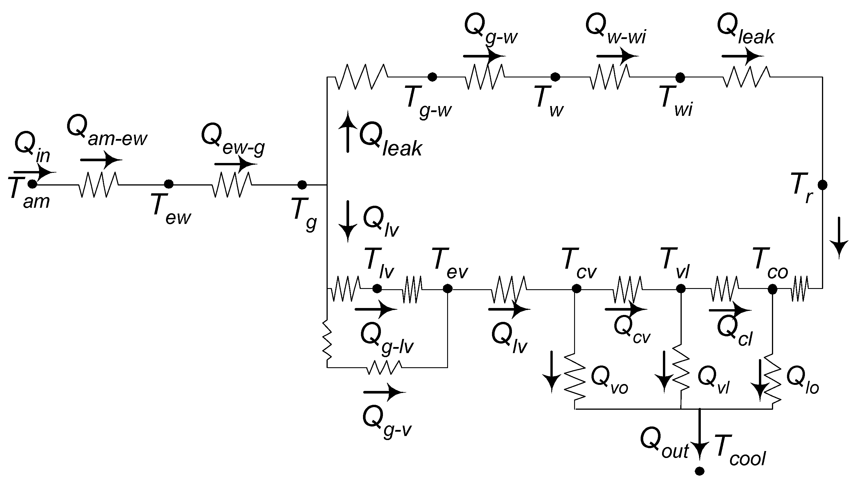
The lumped-layer model [28], which is based on the nodal approach, was used for mathematical-model simplification. Accordingly, the temperature and thermal-flow relationships can be effectively illustrated using the thermal-circuit analogy depicted in Figure 2. Vapor temperature within the vapor-removal groove were estimated via exclusive consideration of convective heat transfer.

The kinetic theory of gases and liquid thin-film theory were used to calculate the phase-change mass flow rate, interface temperature, equilibrium pressure, capillary pressure, and disjoining pressure across the liquid–vapor interface of the evaporator. Via consideration of the energy-conservation principle, the input thermal load applied at the evaporator was evaluated as the sum of the working-fluid latent heat and the sensible heat leaking into the liquid reservoir. The phase-change interface temperature of the condenser was also obtained via consideration of energy conservation between the condensation and evaporation interfaces within the condenser and evaporator, respectively. The working-fluid flow within the condenser was considered to be single-phase (i.e., either pure liquid or pure vapor) based on the condensation interface. The heat-transfer performance of the condenser path was evaluated based on the effectiveness-NTU method, which is widely employed in analysis of heat exchangers.

2.1. Heat-Transfer Modeling of Evaporator

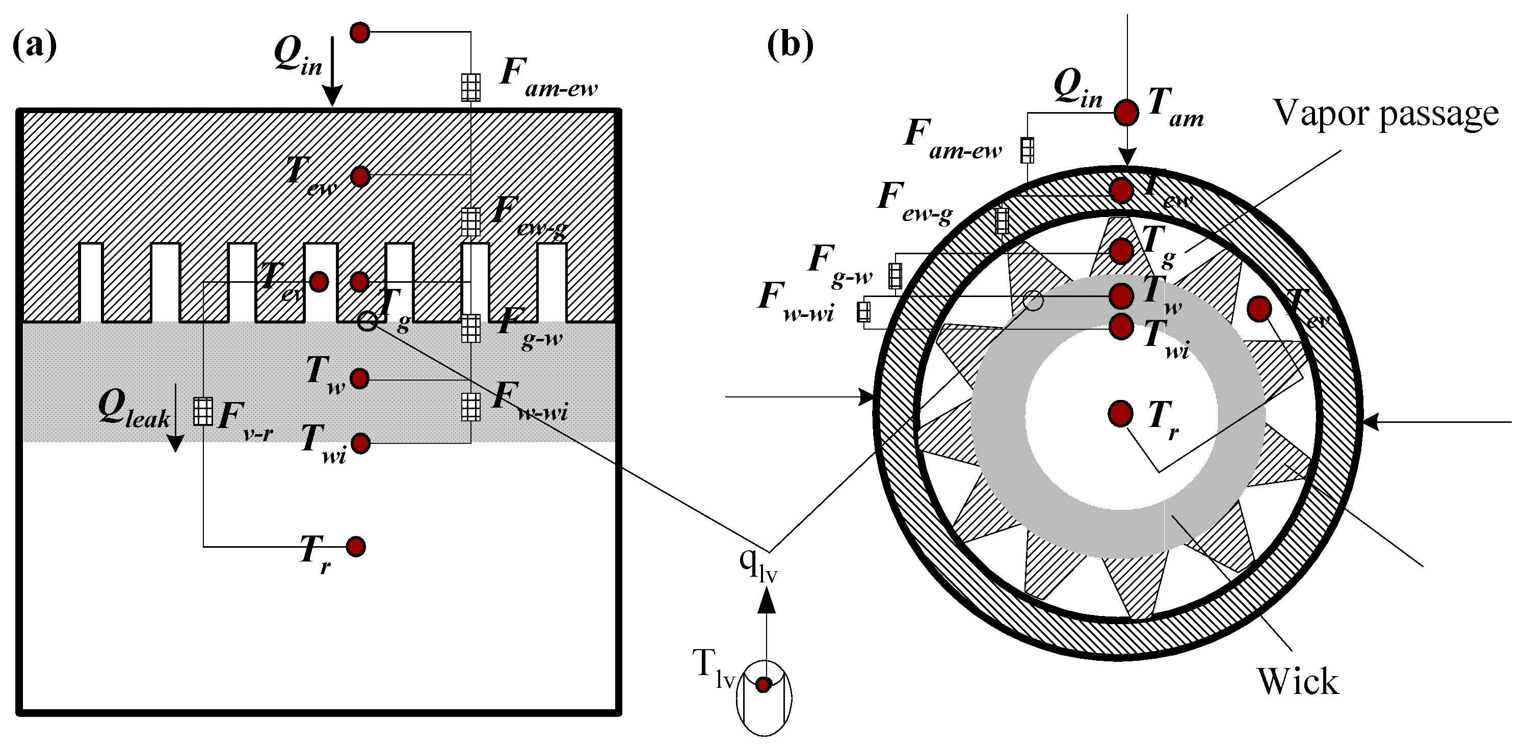
As depicted in Figure 2, the evaporator boundary condition in one-dimensional thermal flow usually corresponds to one of the three types—constant thermal load (Q_in) condition, constant-temperature (T_ew) condition, or convection condition (T_am, U_am). Figure 3 depicts cross sections A–A corresponding to the FLHP and CLHP cases, depicted in Figure 1, as well as the thermal conductance between node temperatures of the thermal circuit depicted in Figure 2. The equation below, in general, pertains to the flow of heat between ambient air and evaporator wall.

$$Q_{am-ew}=F_{am-ew}(T_{am}-T_{ew})=Q_{in},$$

(1)

where F_am-ew denotes the thermal conductance between ambient air and the evaporator wall. Detailed equations concerning the determination of thermal conductance, including Eqution (1), are listed in

Table 1. Thermal conductance values concerning the analytical model of an LHP.

Item	Expression
	FLHP	CLHP
$F_{am-ew}$	$\frac{2k_{ew}{W}_e{L}_e}{t_{ew}}+U_{am}{W}_e{L}_e$	$2\pi r_o{L}_e{U}_{am}+\left[2\pi \left(r_o-\frac{t_{ew}}{2}\right)L_e\right]\frac{2k_{ew}}{t_{ew}}$
$F_{ew-g}$	$\begin{array}{l}\left(\frac{2k_{ew}{W}_e{L}_e}{t_{ew}}+\frac{2k_{geff}{N}_g{W}_g{L}_g}{t_g}\right)+\\ h_g{t}_g{W}_g{N}_g+{\dot{m}}_v{c}_{pv}\end{array}$	$\begin{array}{l}2\pi L_e\left(r_o-t_{ew}-\frac{t_g}{2}\right)\left(\frac{2k_s}{t_{ew}}+\frac{2k_{geff}}{t_g}\right)+\\ h_g\left(\frac{2\pi (r_o-t_{ew})}{N_g}+t_g\right)L_g{N}_g+{\dot{m}}_v{c}_{pv}\end{array}$
$F_{g-w}$	$\begin{array}{l}\left(\frac{2k_{geff}{W}_g{L}_g{N}_g}{t_g}+\frac{2k_{weff}{W}_w{L}_w}{t_g}\right)+\\ h_g{t}_g{W}_g{N}_g+h_w\left(\phi L_w{W}_w\right)+{\dot{m}}_l{c}_{pl}\end{array}$	$\begin{array}{l}2\pi L_e\left(r_o-t_{ew}-t_g-\frac{t_w}{2}\right)\left(\frac{2k_{geff}}{t_g}+\frac{2k_{weff}}{t_w}\right)\\ +h_g{t}_g{L}_e{N}_g+\\ h_w\left[2\pi \phi L_w\left(r_o-t_{ew}-t_g-\frac{t_w}{2}\right)\right]+\\ {\dot{m}}_l{c}_{pv}+{\dot{m}}_l{c}_{pl}\end{array}$
$F_{w-wi}$	$\left(\frac{2k_{weff}{W}_w{L}_w}{t_w}\right)+h_w\left(\phi L_w{W}_w\right)+{\dot{m}}_l{c}_{pl}$	$\begin{array}{l}2\pi L_w\left(r_o-t_{ew}-t_g-t_w\right)\left(\frac{2k_{weff}}{t_w}\right)+\\ h_w\left[2\pi \left(r_o-t_{ew}-t_g-t_w\right)\phi L_w\right]+{\dot{m}}_l{c}_{pl}\end{array}$
$k_{weff}$	$\frac{k_w\left[2k_w+k_l-2\phi \left(k_w-k_l\right)\right]}{2k_w+k_l+\phi \left(k_w-k_l\right)}$

. Similar to Equation (1), the heat flow from evaporator walls to the vapor-removal groove can be expressed as

$$Q_{ew-g}=F_{ew-g}(T_{ew}-T_g),$$

(2)

where T_g is the groove temperature. As described in Table 1, the term F_ew-g further corresponds to a combination of $k_{geff}\left[=\varphi k_v+(1-\varphi )k_g\right]$—the effective thermal conductivity with due consideration of the groove porosity (φ)—as well as $h_g\left[=k_{v}N{u}_g/D_{h,g}\right]$—the convective heat-transfer coefficient between the vapor and groove. Nu_g denotes the Nusselt number defined by the groove geometry and corresponding flow characteristics. In this study, the value of Nu_g for fully developed laminar flow through a flow path characterized by trapezoidal cross sections was set to 7.57 [32]. The term D_hg denotes hydraulic diameter of the vapor-removal groove.

The vapor temperature within the evaporator (T_ev) can be expressed as

$$T_{ev}=T_g-\frac{Q_{ew-g}}{h_g{A}_g}.$$

(3)

As described in Equation (3), T_ev can be separately determined considering convective heat transfer between the groove and vapor temperature.

Through energy conservation, part of the thermal energy transferred to the groove wall can be utilized during evaporation of the working fluid, and the rest can be leaked into the liquid reservoir via conduction and convection. The latter does not correspond to an ideal approach; however, the said leakage from an evaporator structure cannot be avoided in practice. Below is the energy conservation equation associated with this phenomenon.

$$Q_{ew-g}=Q_{lv}+Q_{g-w},$$

(4)

where Q_lv denotes the rate of phase-change heat transfer associated with the latent heat of vaporization, and Q_q-w represents the heat leak toward the liquid reservoir.

The heat-transfer coefficient corresponding to the phase change within pores of the wick can be denoted by h_lv, and the corresponding heat-transfer rate can be expressed as

$$Q_{lv}=h_{lv}{A}_{lv}\Delta T=h_{lv}\phi A_w\Delta T,$$

(5)

where A_lv is the evaporation-interface area, which can be estimated by the product of the porosity of the wick (φ) and apparent wick surface area (A_w), i.e., $A_{lv}\approx \phi A_w$ as reflected in the equation. ΔT denotes the temperature difference across the phase interface. The pores of the wick are assumed to be fully saturated with liquid.

Assuming the capillary structure to be saturated with liquid and the liquid–vapor interface to be located on the contact surface between the vapor-removal groove and wick, Q_q-w can be expressed as,

$$Q_{g-w}=F_{g-w}(T_g-T_w),$$

(6)

where T_w represents the temperature of the wick in contact with the groove. The thermal conductance F_g-w in Equation (6) involves the effective thermal conductivity of the liquid-saturated wick, k_weff, and the convective heat-transfer coefficient between the adjacent liquid, h_w (see Table 1).

Moreover, the heat-transfer coefficient associated with heat flow from the evaporation surface to the adjacent liquid can be expressed as

$$h_w=Q_{g-w}/A_{lv}(T_{g-w}-T_{el}),$$

(7)

where T_g-w denotes the temperature of the wick near the surface in contact with the groove, and the same can be determined as the arithmetic mean of T_g and T_ev. T_el denotes the liquid temperature near the interface, which is practically difficult to determine. The above liquid and vapor temperatures (T_el and T_ev, respectively) across the interface are nearly identical if the working fluid is in saturated state during evaporation.

Across the capillary wick, the heat-transfer rate from the liquid near the evaporation surface to its sub-cooled counterpart inside the liquid reservoir can be expressed as

$$Q_{w-wi}=F_{w-wi}(T_w-T_{wi})=Q_{g-w}=Q_{leak},$$

(8)

where Q_leak denotes the thermal energy eventually transferred to the liquid reservoir. As shown in Figure 2 and Figure 3, the definition of Q_leak is essential to understand the flow of heat energy to predict the heat transfer performance of the LHP. Launay et al. [23] presented the expression of Q_leak for FLHP and CLHP as Equations (9) and (10), respectively. For the FLHP,

$$Q_{leak}={\dot{m}}_l{c}_{pl}(T_{ev}-T_r)/\left\{\exp \left[\frac{{\dot{m}}_l{c}_{pl}{t}_w}{k_{weff}{A}_w}\right]-1\right\}$$

(9)

and for the CLHP, Q_leak can be expressed as

$$Q_{leak}={\left(\frac{d_{wi}}{d_{wo}}\right)}^{\frac{{\dot{m}}_l{c}_{pl}}{2\pi k_{weff}{t}_w}}\left[\frac{{\dot{m}}_l{c}_{pl}}{1-{\left(\frac{d_{wi}}{d_{wo}}\right)}^{\frac{{\dot{m}}_l{c}_{pl}}{2\pi k_{weff}{t}_w}}}\right](T_{ev}-T_r),$$

(10)

where d_wo and d_wi denote outer and inner diameters of the wick structure, respectively.

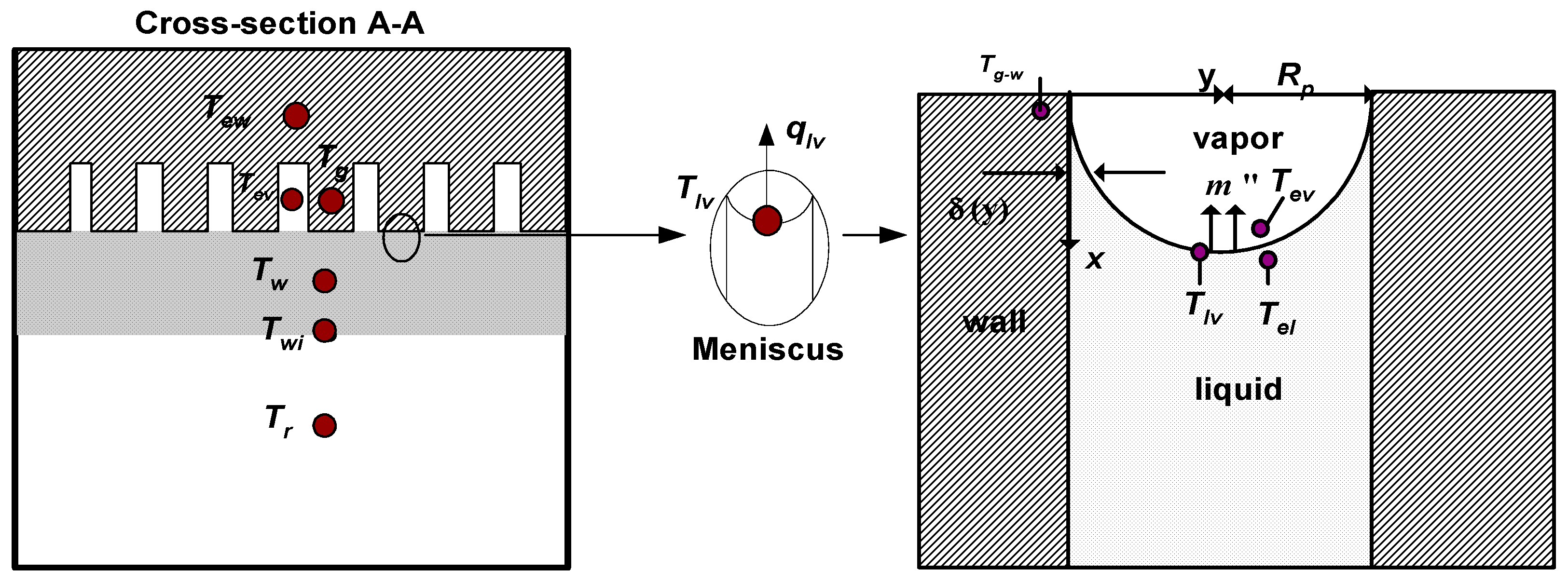
2.2. Phase-Change Modeling on Evaporation Surface

In this study, as previously mentioned, the configuration of and temperature across the liquid–vapor interface were determined using the liquid thin-film theory [33]. Figure 4 shows the configuration and physical parameters for the evaporation interface of a single pore with cylindrical shape in the capillary structure.

The behavior of the vapor–liquid interface is dominated by the pressure difference between the liquid and vapor phases. The pressure difference can be expressed through an augmented Young–Laplace equation, which is given as the sum of the capillary and disjoining pressure.

$$p_{ev}-p_l=p_d+p_c,$$

(11)

where, p_ev and p_l denotes the evaporator vapor and liquid pressures. p_d and p_c represent the disjoining pressure and capillary pressure, respectively.

The interface curvature is created by the liquid surface tension and capillary structure. The corresponding capillary pressure (p_c) within the pores, in accordance with the liquid thin-film theory, can be expressed as [33]:

$$p_c=\sigma K,K=\frac{d^2\delta }{d{x}^2}{\left[1+{\left(\frac{d\delta }{dx}\right)}^2\right]}^{-1.5},$$

(12)

where K and σ denote the interface curvature and surface tension, respectively; and dδ/dx denotes the derivative of the liquid thin-film thickness with respect to x, as depicted in Figure 4.

The disjoining pressure can be approximated as a function of the liquid-film thickness [34]:

$$p_d=\frac{H}{{\delta }^3},$$

(13)

where H denotes the dispersion (or Hamaker) constant. When employing methanol as the working fluid, H equals −1.07 × 10⁻¹⁹ J [33].

In addition, δ denotes thickness of the liquid thin-film thickness, the maximum value of which corresponds to the pore radius. The detailed representation of the Young–Laplace equation appears as a fourth-order ordinary differential equation, which can be solved using the method proposed by Wang et al. [34]. Once the solution is obtained, the liquid thin-film thickness and film configuration can be obtained.

The mass flow rate during slow phase-change of the evaporative processes can be expressed as [29]:

$$m_{lv}^{″}=\beta \gamma \left(\frac{p_{eq}}{T_{lv}^{1/2}}-\frac{p_{ev}}{T_{ev}^{1/2}}\right),$$

(14)

where β = 2α/(2 − α) and $\gamma =\sqrt{\overline{M}/2\pi \overline{R}}$; $\overline{M}$ denotes the molecular weight; and $\overline{R}$ denotes the universal gas constant. For water, ethanol, and methanol, values assumed by the accommodation coefficient (α) lie within the range of 0.002–0.004. The equilibrium pressure (p_eq) of the phase-change interface can be determined using the equation below [29].

$$p_{eq}(T_{lv})=p_{sat}(T_{lv})\exp \left[\frac{p_{lv-equ}-p_{sat}(T_{lv})-(p_d+p_c)}{{\rho }_l{T}_{lv}\overline{M}/\overline{R}}\right].$$

(15)

In the above equation, the saturation pressure ($p_{sat}(T_{lv})$) corresponding to the interface temperature can be determined using the following equation [29].

$$p_{sat}(T_{lv})=p_{sat\_ref}(T_{sat\_ref})\exp \left[\frac{\overline{M}{h}_{fg}}{\overline{R}}\left(\frac{1}{T_{sat\_ref}}-\frac{1}{T_{lv}}\right)\right].$$

(16)

Given a saturated interface with saturation pressure [= p_sat(T_lv) = p_{sat_ref}(T_{sat_ref})], the corresponding superheated state could be arbitrarily considered to correspond to T_{sat_ref} = T_lv − T_super, where T_super denotes superheat temperature.

The rate of conductive heat transfer across the liquid thin-film to the vapor can be determined by Equation (17).

$$m_{lv}^{″}{h}_{fg}=k_l(T_{g-v}-T_{lv})/\delta .$$

(17)

Using Equations (14) and (17), the phase-change temperature at the evaporation interface can be expressed as follows [34].

$$T_{lv}=T_{g-v}+\frac{\delta }{k_l}\beta \frac{h_{fg}}{\gamma }\left[\frac{p_{eq}}{T_{lv}^{1/2}}-\frac{p_{ev}}{T_v^{1/2}}\right].$$

(18)

The heat transfer rate by vaporization was defined as Equation (19) through the linearization process of Equation (14) [29].

$$Q_{lv}=A_{lv}{m}_{lv}^{″}{h}_{fg}={\left\{A_{lv}\left(\frac{2\alpha }{2-\alpha }\right)\frac{h_{fg}^2}{T_{ev}{v}_{fg}}\sqrt{\frac{\overline{M}}{2\pi \overline{R}\left(T_v\right)}}\left[1-\frac{p_v{v}_{fg}}{2h_{fg}}\right](T_{lv}-T_{ev})\right\}}_e.$$

(19)

As shown in Equation (19), if the temperatures at the evaporation interface and that of the vapor are known, Q_lv can be determined. Alternatively, since Q_lv is also obtained by the phase change mass flow rate, latent heat and evaporative heat transfer area in the evaporator, the temperature and configuration [34] of the phase change interface generated in the fine pores of the capillary structure should be defined. Q_lv is the thermal energy that is transferred to the condenser, and when this value is obtained, it is possible to analyze the heat transfer to the condenser path.

2.3. Phase-Change Modeling on Condensation Surface

Similar to Equation (19), the observed heat-transfer rate due to condensation can be expressed as [29]:

$$Q_{vl}=A_{vl}{m}_{vl}^{″}{h}_{fg}={\left\{A_{vl}\left(\frac{2\alpha }{2-\alpha }\right)\frac{h_{fg}^2}{T_{cv}{v}_{fg}}\sqrt{\frac{\overline{M}}{2\pi \overline{R}\left(T_v\right)}}\left[1-\frac{p_v{v}_{fg}}{2h_{fg}}\right](T_{cv}-T_{vl})\right\}}_c,$$

(20)

where T_cv denotes the temperature of the vapor at the condenser inlet, and T_vl represents the temperature at the condensation interface.

The condenser inlet vapor temperature can be expressed as T_cv = T_ev − δT, where δT refers to the temperature drop caused by the vapor path in the condenser, which in turn, depends on cooling conditions. Assuming the generation of a condensation interface between the vapor and liquid phases at any position within the condenser path [30], the condensation-interface temperature can be evaluated using Equations (21) and (22) based on the energy-conservation relation between the evaporation and condensation interfaces. Additionally, assuming that the condensation interface is flat, the term A_vl can be considered as the cross-sectional area of the condenser path. Equation (21) was deduced assuming the evaporative and condensation heat transfer rates (Q_lv and Q_vl, respectively) to be identical within the closed loop.

$$\frac{Q_{lv}}{Q_{vl}}=\left(\frac{A_{lv}}{A_{vl}}\right)\frac{{\left(\frac{h_{fg}^2}{T_{ev}{v}_{fg}}\right)}_e}{{\left(\frac{h_{fg}^2}{T_{cv}{v}_{fg}}\right)}_c}\frac{\sqrt{\frac{M}{2\pi R_v{T}_{ev}}}}{\sqrt{\frac{M}{2\pi R_v{T}_{cv}}}}\frac{{\left[1-\frac{p_{ev}{v}_{fg}}{2h_{fg}}\right]}_e}{{\left[1-\frac{p_{cv}{v}_{fg}}{2h_{fg}}\right]}_c}\frac{(T_{lv}-T_{ev})}{(T_{cv}-T_{vl})}=1.$$

(21)

The above equation can be arranged for T_vl, as shown in Equation (22).

$$T_{vl}=T_{cv}-\left(\frac{A_{lv}}{A_{vl}}\right)\frac{{\left(\frac{h_{fg}^2}{T_{ev}{v}_{fg}}\right)}_e}{{\left(\frac{h_{fg}^2}{T_{cv}{v}_{fg}}\right)}_c}\frac{\sqrt{\frac{\overline{M}}{2\pi R_v{T}_{ev}}}}{\sqrt{\frac{\overline{M}}{2\pi R_v{T}_{cv}}}}\frac{{\left[1-\frac{p_{ev}{v}_{fg}}{2h_{fg}}\right]}_e}{{\left[1-\frac{p_{cv}{v}_{fg}}{2h_{fg}}\right]}_c}(T_{lv}-T_{ev}).$$

(22)

Once the condensation interface temperature is obtained, the condenser flow path can be hypothetically divided into a vapor region and a liquid region, and the length of the vapor and liquid regions can be predicted by conventional heat exchanger theories.

The heat flows associated with condenser are shown in Figure 2. Among the heat flows that appear in the paths along the condenser, Q_cv and Q_cl correspond to $\dot{m}{c}_{pv}\left(T_{cv}-T_{vl}\right)$ and $\dot{m}{c}_{pl}\left(T_{vl}-T_{co}\right)$, respectively. On the other hand, the heat flows from the condenser to the coolant (heat sink), Q_vo and Q_lo are the sensible heat removal from the vapor phase and liquid phase, respectively, before and after the vapor-to-liquid phase change. The other heat removal, Q_vl, occurs during the condensation, as described by Equation (20).

The condenser length occupied by vapor (L_cv) can subsequently be determined using in Equation (23), which was deduced using the NTU–ε method [35] as part of the heat-exchanger analysis.

$$L_{cv}=\frac{NT{U}_{cv}\times C_{\min }}{P\times U_{cv}}.$$

(23)

Thence, the corresponding length of the liquid portion can, obviously, be determined using the relation L_cl = L_c − L_cv, where L_c denotes the total condenser length. Once L_cv and L_cl are determined, Q_vo and Q_lo can be easily obtained by the heat exchanger analysis theory [35].

The liquid temperature at condenser outlet can be determined using the following equation.

$$T_{co}=T_{vl}-{\epsilon }_{cl}\frac{C_{\min }}{C_l}(T_{vl}-T_{cool.in}).$$

(24)

The heat transfer rate caused by the temperature difference between the condenser outlet and liquid reservoir, $\dot{m}{c}_{pl}\left(T_r-T_{co}\right)$, can be identified as the leakage heat, Q_leak, which was also expressed by Equations (8)–(10). Combining these equations, the liquid reservoir temperature can be determined.

For the FLHP, the temperature in the liquid reservoir can be expressed as

$$T_r=\frac{\frac{\dot{m}{c}_{pl}}{{\left(\exp \left[\frac{\dot{m}{c}_{pl}{t}_w}{k_{weff}{A}_w}\right]\right)}_e-1}{T}_{ev}+{\left(\dot{m}{c}_{pl}\right)}_c{T}_{co}}{\frac{\dot{m}{c}_{pl}}{{\left(\exp \left[\frac{\dot{m}{c}_{pl}{t}_w}{k_{weff}{A}_w}\right]\right)}_e-1}+{\left(\dot{m}{c}_{pl}\right)}_c}$$

(25)

In addition, for the CLHP, the temperature in the liquid reservoir can be expressed as

$$T_r=\frac{{\left[\frac{\dot{m}{c}_{pl}{\left(\frac{d_{wi}}{d_{wo}}\right)}^{\raisebox{1ex}{$\dot{m}{c}_{pl}$}\!\left/ \!\raisebox{-1ex}{$2\pi k_{weff}{L}_w$}\right.}}{1-{\left(\frac{d_{wi}}{d_{wo}}\right)}^{\raisebox{1ex}{$\dot{m}{c}_{pl}$}\!\left/ \!\raisebox{-1ex}{$2\pi k_{weff}{L}_w$}\right.}}\right]}_e{T}_{ev}+{\left(\dot{m}{c}_{pl}\right)}_c{T}_{co}}{{\left[\frac{\dot{m}{c}_{pl}{\left(\frac{d_{wi}}{d_{wo}}\right)}^{\raisebox{1ex}{$\dot{m}{c}_{pl}$}\!\left/ \!\raisebox{-1ex}{$2\pi k_{weff}{L}_w$}\right.}}{1-{\left(\frac{d_{wi}}{d_{wo}}\right)}^{\raisebox{1ex}{$\dot{m}{c}_{pl}$}\!\left/ \!\raisebox{-1ex}{$2\pi k_{weff}{L}_w$}\right.}}\right]}_e+{\left(\dot{m}{c}_{pl}\right)}_c}.$$

(26)

The overall heat-transfer coefficient (U_am) between the evaporator wall and ambient air can, therefore, be expressed in the thermal-resistance form as

$$\frac{1}{U_{am}{A}_c}=\frac{1}{F_{am-ew}}+\frac{1}{F_{ew-g}}+\frac{{\left(\frac{1}{UA}\right)}_{cv}+{\left(\frac{1}{UA}\right)}_{cl}}{2}+\frac{1}{F_{g-w}}+\frac{1}{F_{w-wi}}+\frac{1}{h_w{A}_{lv}}.$$

(27)

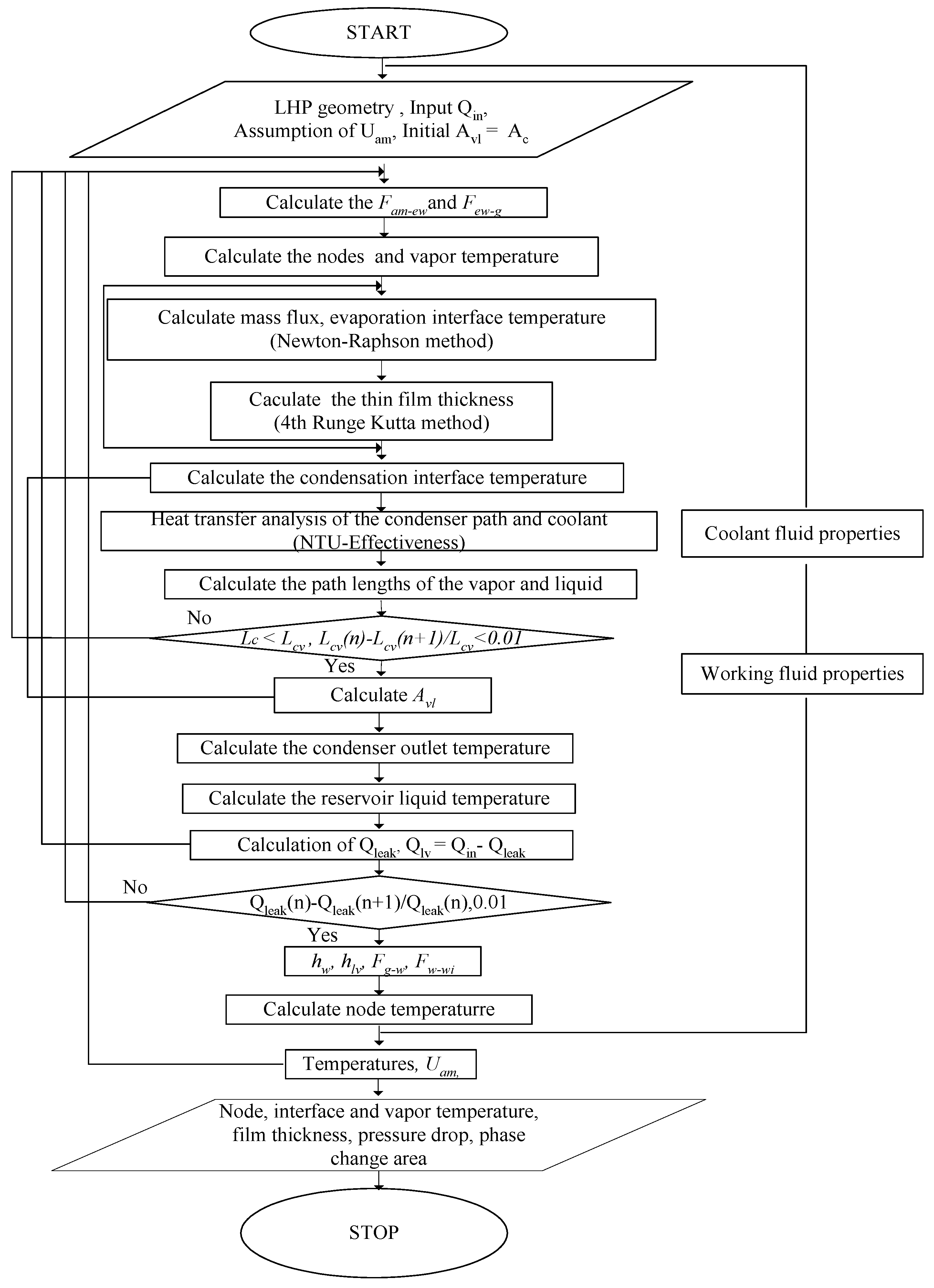
In the prosed study, an initial estimate of U_am is made at the beginning of the heat-transfer analysis. Subsequently, relevant calculations are repeatedly performed, until converged values are attained for all the temperatures at different locations. Ultimately, the value of U_am was iteratively determined using Equation (27) until the initially estimated and calculated values were converged with sufficiently small difference. A flow chart demonstrating the above calculation process is depicted in Figure 5.

3. Results and Discussion

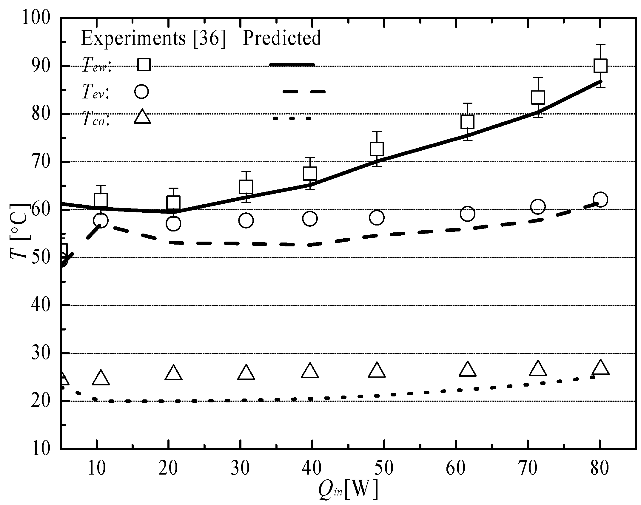
To demonstrate the validity of the analytical model, the predicted results were compared with the experimental results. Figure 6 illustrates the model prediction against the corresponding experimental data for a FLHP with methanol as a working fluid [36]. As representative temperatures, those of the evaporator wall (T_ew), evaporator vapor (T_ev), and condenser outlet (T_co) were investigated for the input thermal load the range of 10 to 80 W. The predicted value of the wall temperature of the evaporator was in close agreement with the experimental result within the relative error of 0.5%. It was presumed that the error might have been very small because the overall heat transfer coefficient, U_am, was determined by the experimental results. The relative error of the vapor temperature was 1.2% at the maximum (thermal load of 40 W), and the errors for all the other input thermal loads were less than 0.8%. From these results, it was confirmed that the heat transfer coefficient (h_g) used in the model was appropriate. For thermal loads between 20 and 40 W, the predicted value of the liquid temperature at the condenser outlet exhibited relatively large error compared to other temperatures, but the temperature error was less than 4 °C. On the other hand, for an input heat load of 80 W, the predicted values nearly coincided with experiments with only little error.

With regard to investigating the effect of LHP design variables on LHP heat transfer performance, FLHP was considered as the basic model [36], geometric dimensions of which are depicted in

Table 2. FLHP geometric characteristics and working conditions.

LHP Dimensions/Working Condition	FLHP by Boo and Chung [36]
Working fluids	Methanol
LHP-case material	Stainless steel 316 L
Evaporator	50 (Le) × 40 (We) × 30 (He) mm
Trapezoidal vapor-removal groove	3 (tg) × 3 (Wg) mm, 75°(θ)
Number of axial grooves	9
Wick material/porosity/pore diameter	Stainless steel/47%/0.5 µm
Wick dimensions	5 mm (tw)
Liquid/vapor-line dimension	2 mm (dpi)/4 mm(dpi), 0.5 m (L)
Condenser	Rectangular, 4 (Wc) × 5 (Lc) cm
Liquid-reservoir volume	35.5 mL
Coolant temperature	0, 10, 20, 30 °C
Coolant	Mixture of 80% water and 20% ethylene-glycol, 5GPH
Ambient temperature	20~25 °C

. The evaporator and condenser dimensions of the said model were identical to those described in [36]. However, basic specifications of the capillary structure were defined differently to include stainless steel (STS 316L) as its base material with 47% porosity (φ) and a sintered metal particle diameter of 5 µm. During the said investigation, porosity (φ) of the capillary structure, temperature drop due to relevant cooling conditions (δT), and number of turns (n) of the condenser path were considered to be primary design variables.

During simulations performed to evaluate heat-transfer performance of LHP, the different design variables were assigned the following values. The temperature drop (δT) due to cooling conditions equaled 0 °C; coolant inlet temperature (T_cool,,in) was set to 10 °C; superheat temperature (T_super) was set to 0 °C; particle diameter of porous structure was set as 5 µm; capillary-structure porosity (φ) equaled 0.6; and the number of turns (n) of the condenser path was set as 5. It must be noted that two of the straight configurations in the crooked condenser path in Figure 1b correspond to one turn.

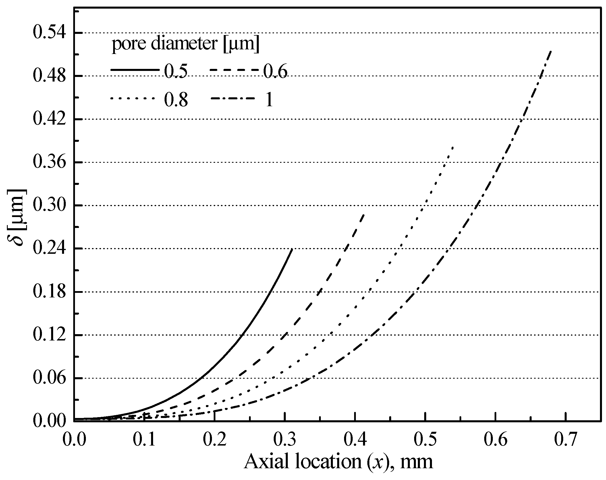
Figure 7 and Figure 8 demonstrate results obtained regarding the prediction of film thickness, capillary pressure, and disjoining pressure in accordance with changes in pore size of the capillary structure. The said predictions were performed via application of the thin-film theory [34] to the pores of the wick depicted in Figure 4. The above-mentioned results were depicted as functions of the pore diameter. The geometric configuration of the LHP used during analysis was identical to those described in [34].

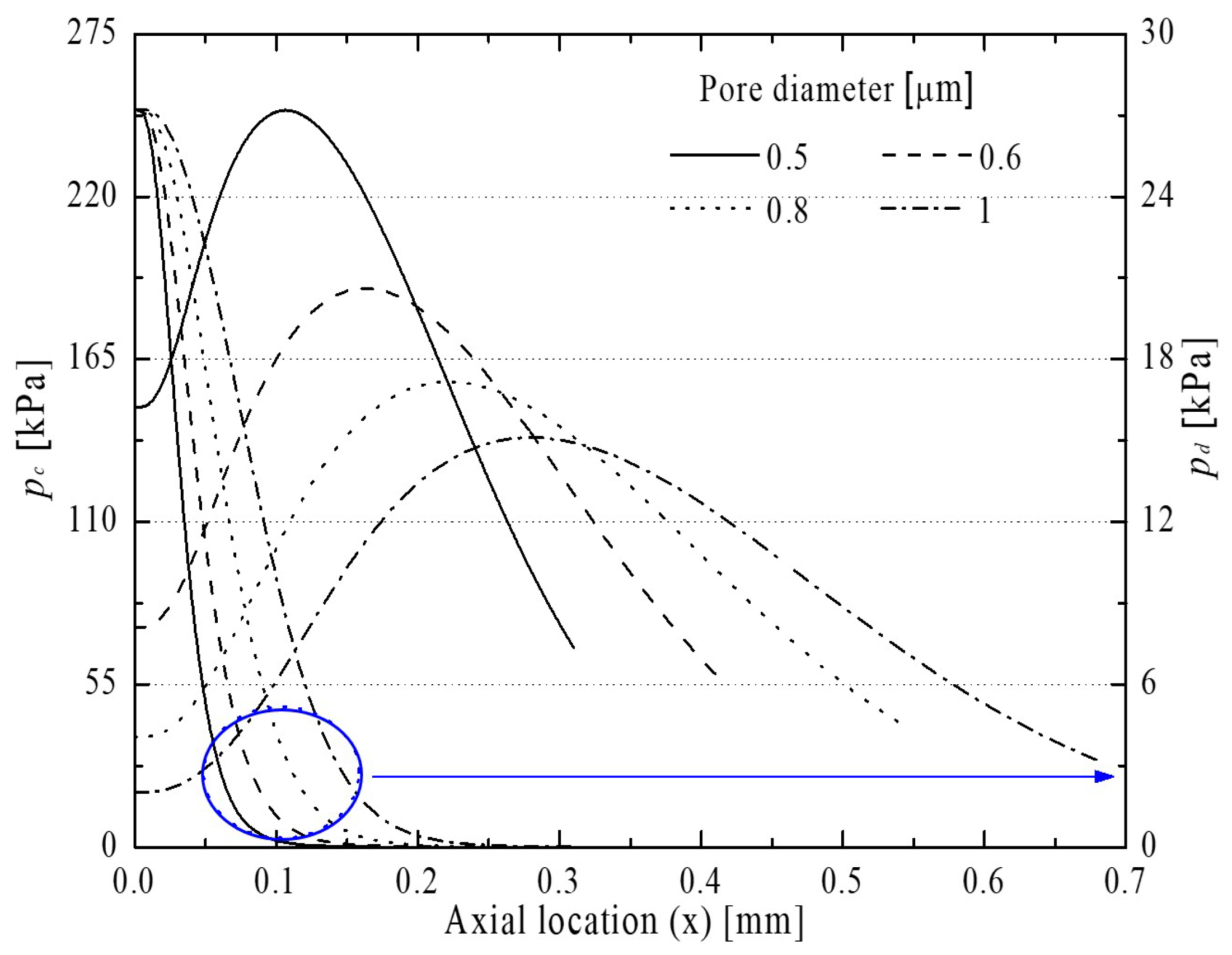
As depicted in Figure 7, with increase in pore size, thickness of the liquid film reduces at the same axial location (i.e., along the x-axis in Figure 4). For example, when the pore diameter equaled 0.5 µm, the corresponding film thickness equaled approximately 0.25 µm at x = 0.3 µm, whereas at a pore diameter of 1 µm, the corresponding film thickness was reduced to 0.04 µm. Figure 8 demonstrates an increase in maximum capillary pressure with reduction in pore diameter. As can be observed in the said figure, at pore-diameter values of 0.5 and 1 µm, the maximum capillary pressures correspond to 250 and 140 kPa, respectively. The said pressure values were calculated at a point located midway along the pore radius (denoted by R_p in Figure 4) at which the interface curvature demonstrated its highest value. Additionally, Figure 8 illustrates the disjoining pressure (p_d) to be inversely proportional to the liquid thin-film thickness (δ), as described in Equation (13). The maximum value of p_d corresponds to the commencement of liquid film formation, subsequent to which the value of p_d rapidly reduces to nearly zero. That said, the value of p_d increases with increase in pore diameter. As can be observed in Figure 8, at x = 0.05 µm, p_d equals 2.5 and 240 kPa corresponding to pore-diameter values of 0.5 and 1 µm, respectively.

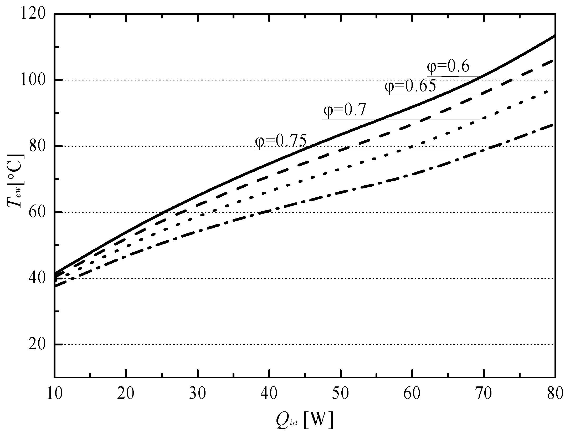
Figure 9 depicts variation trends concerning the T_ew value of LHP in accordance with the increase in Q_in as a function of porosity (φ). The overall heat-transfer coefficient (U_am) between the evaporator outer wall and ambient air was calculated using Equation (27). As can be observed in Figure 9, T_ew decreases corresponding to an increase in φ. This is because if the value of k_weff concerning the capillary structure decreases, values of F_g-w and F_w-wi also subsequently decrease, thereby causing the thermal energy transferred to the condenser to increase, as described in Equations (6) and (8) and Table 1. For example, at Q_in = 80 W, as the value of φ increases from 0.6 to 0.75, that of T_ew is reduced by approximately 27 °C.

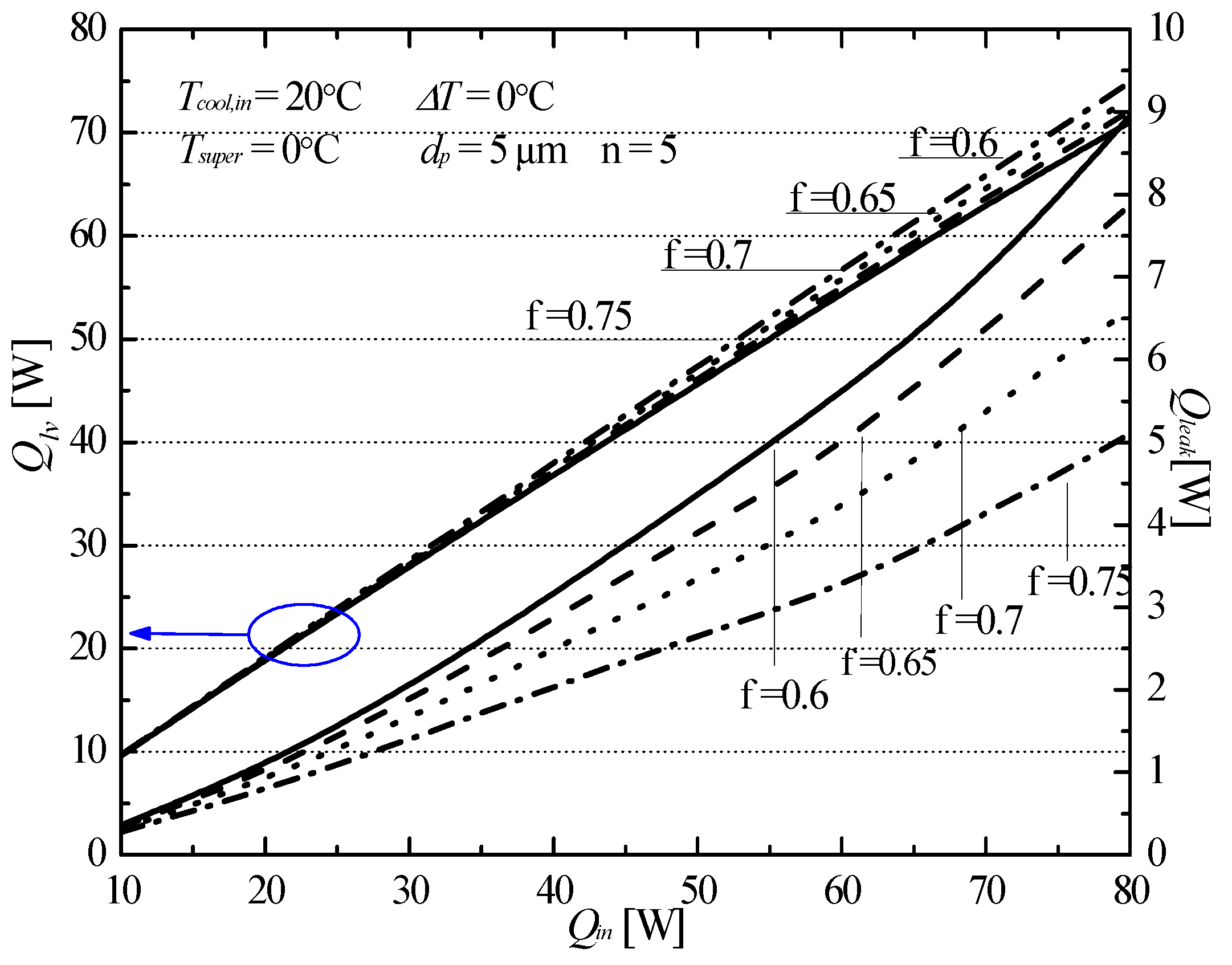
Figure 10 depicts variation trends concerning values of the evaporative heat-transfer rate (Q_lv) and leakage heat (Q_leak)—flowing into the liquid reservoir via the capillary structure—as a function of Q_in whilst corresponding to different values of porosity (φ). From the energy-conservation viewpoint, the relation Q_in = Q_lv + Q_leak must be satisfied at all times. Trends depicted in Figure 10 demonstrate that with increase in porosity (φ), Q_leak decreases, and this causes an increase in Q_lv. For example, at Q_in = 80 W, as φ increases from 0.6 to 0.75, the corresponding value of Q_leak reduces by approximately 2.78 W while that of Q_lv increases by the same amount.

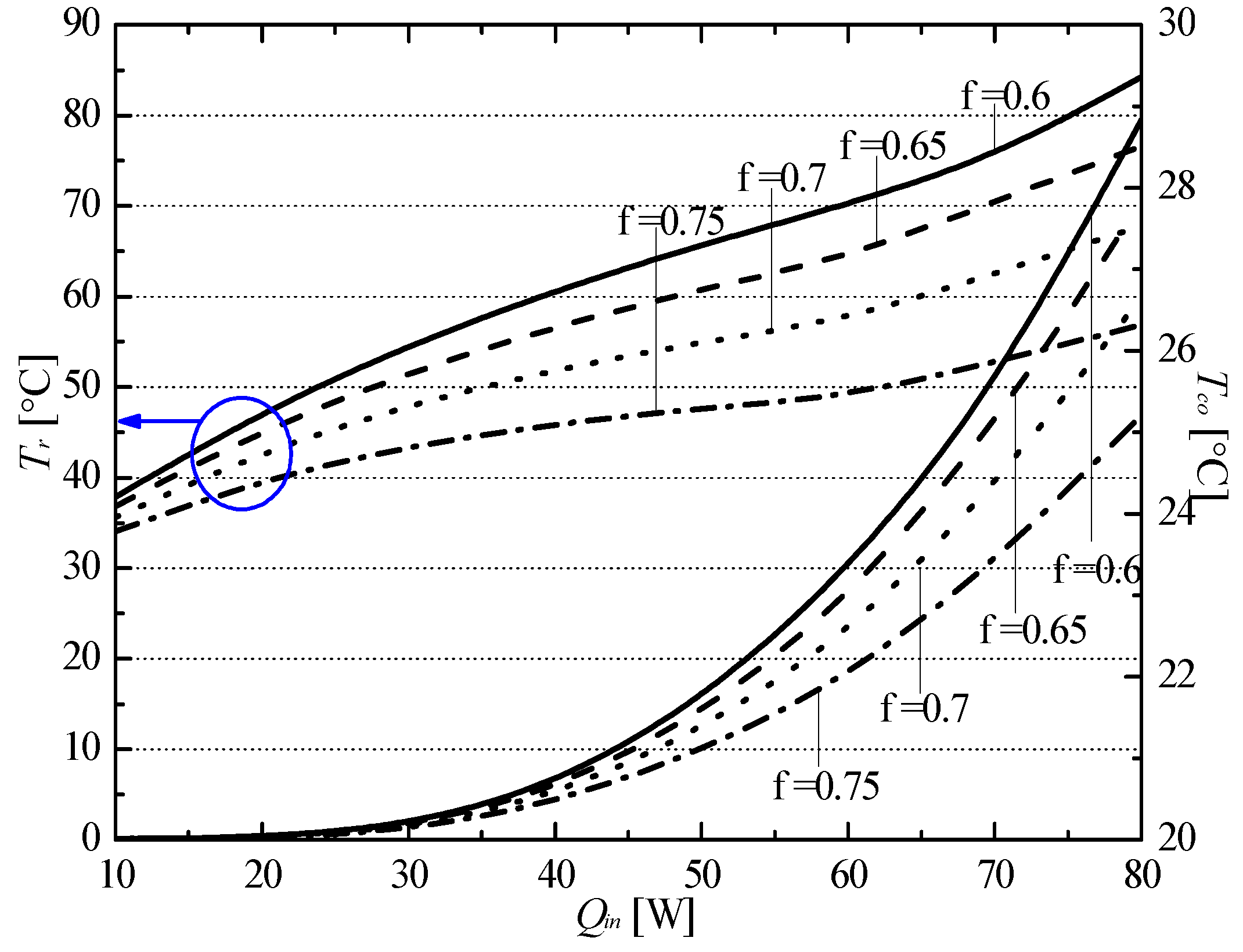
Figure 11 depicts trends concerning variations in the LHP liquid-reservoir and condensate-outlet temperatures (T_r and T_co, respectively) at different porosities (φ) as functions of Q_in. Here, values of T_r and T_co were obtained using Equations (24) and (25). As depicted in Figure 10, values of both T_r and T_co decrease as φ increases. Additionally, as described in Equations (24) and (25), the two temperatures are related to each other, and that a reduction in the vapor temperature ($T_{ev}$) and T_co cause a corresponding reduction in T_r. Any reduction in the heat transfer rate into the liquid reservoir tends to reduce the value of T_ev, thereby resulting in a lower value of T_co. For example, at Q_in = 80 W, as φ increases from 0.6 to 0.75, the corresponding value of T_r reduces by 27.4 °C while that of T_co falls by 3.6 °C.

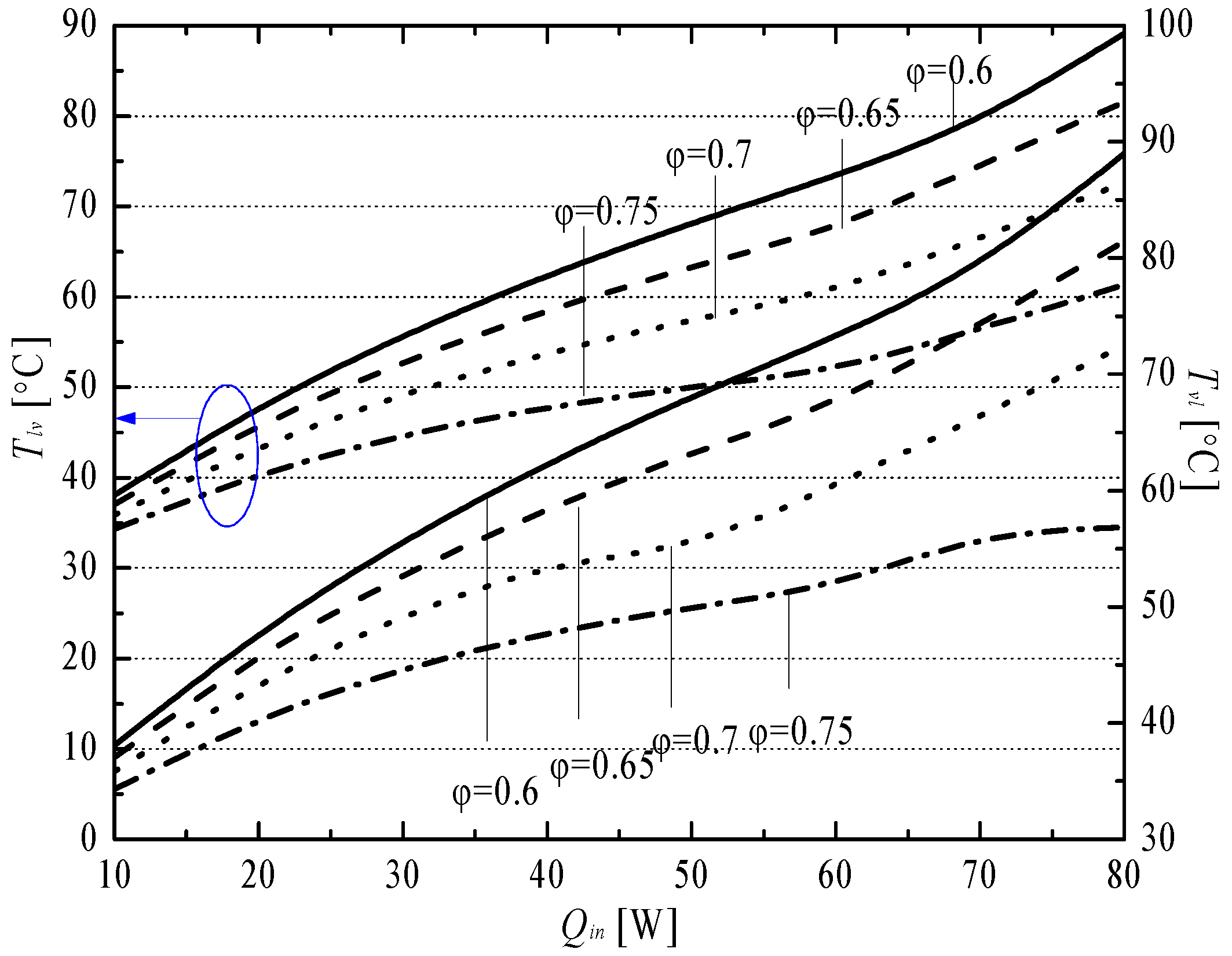
Figure 12 depicts variation trends concerning values of the LHP evaporation- and condensation-interface temperatures (T_lv and T_vl, respectively), at different values of the porosity, as a function of Q_in. As can be seen in the figure, an increase in φ corresponds to reduction in the values of both T_lv and T_vl. As described in Equations (18) and (22), the evaporator-vapor temperature reduces with increase in φ, thereby causing T_lv to decrease. In addition, as described in Equation (22), increase in φ causes a reduction in the interface area ratio (A_lv/A_vl), which in turn, reduces T_vl. At Q_in = 80 W, as φ increases from 0.6 to 0.75, corresponding values of T_lv and T_vl reduce by 27.8 and 32.1 °C, respectively.

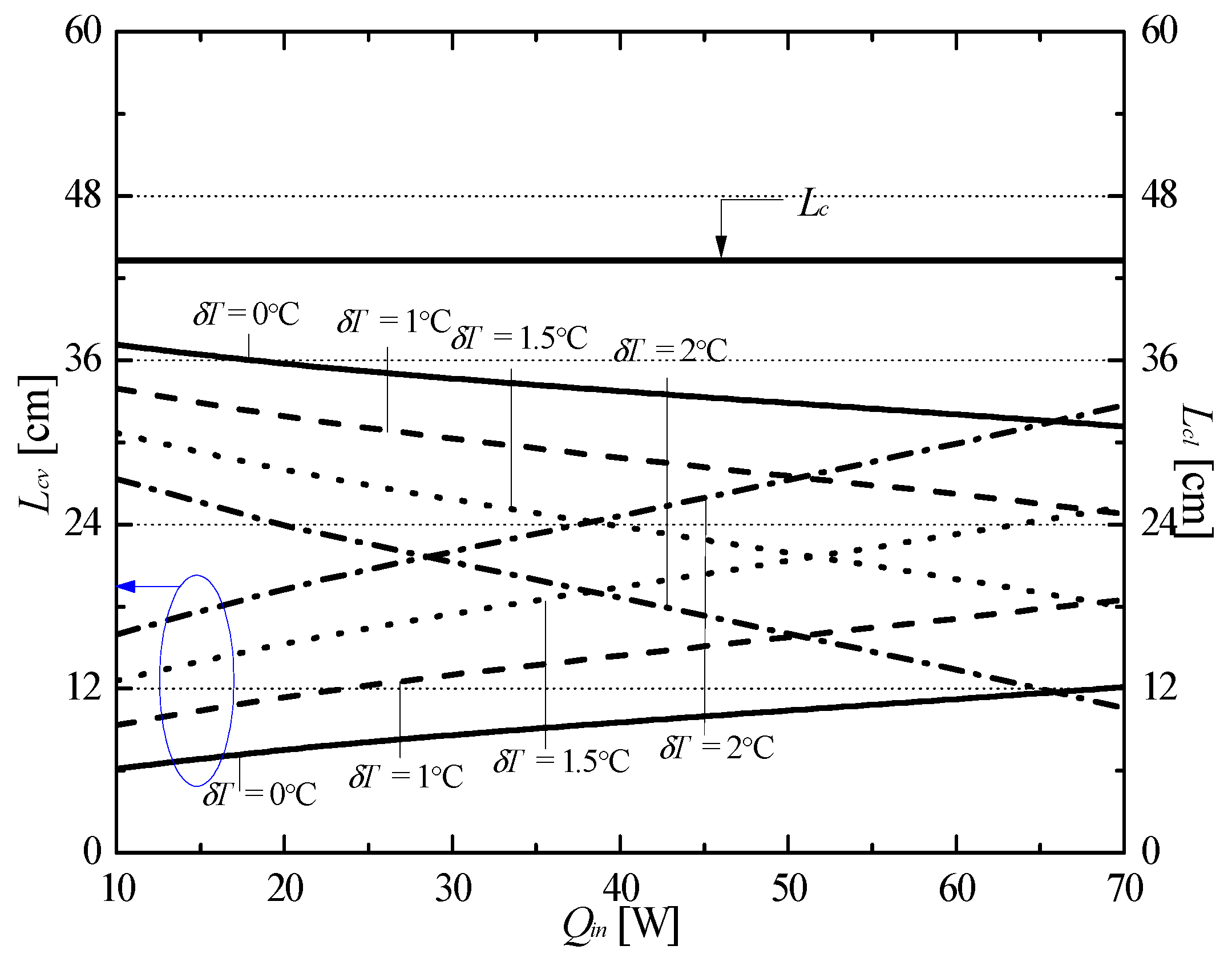
Figure 13 depicts trends concerning changes in lengths of the vapor and liquid paths (L_cv and L_cl, respectively) of the condenser as a function of Q_in for cases involving different values for the drop in vapor temperature (δT). As can be observed in the said figure, the value of L_cv increases with increase in thermal load while that of L_cl [= L_c − L_cv] correspondingly reduces. At Q_in = 70 W, the value of δT increases from 0 to 2 °C; correspondingly values of L_cv and L_cl demonstrate an enhancement and reduction of 20.6 cm, respectively.

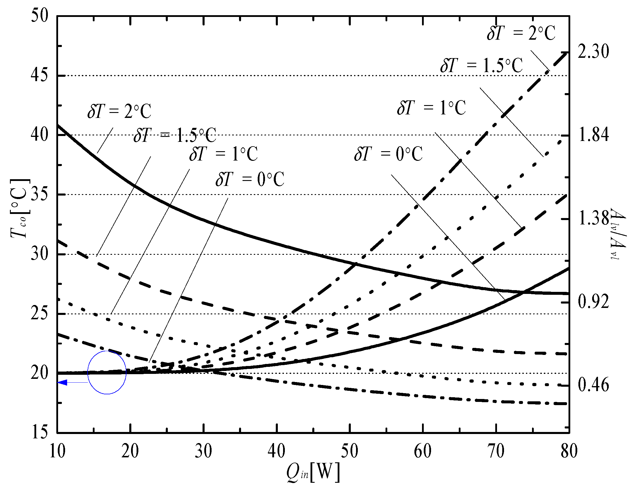
Figure 14 depicts observed trends concerning changes in the condenser-liquid temperature (T_co) and the interface area ratio (A_lv/A_vl) as functions of Q_in for different values of the vapor-temperature drop (δT). As depicted in Figure 14, an increase in Q_in causes values of T_co and A_lv/A_vl to increase and decrease, respectively. In addition, as δT increases, values of both T_co and A_lv/A_vl demonstrate an increase. Corresponding to an input thermal load Q_in = 80 W, as T_co increases from 0 to 2 °C, corresponding values of T_co and A_lv/A_vl increase and decrease by approximately 18.3 °C and 0.61, respectively.

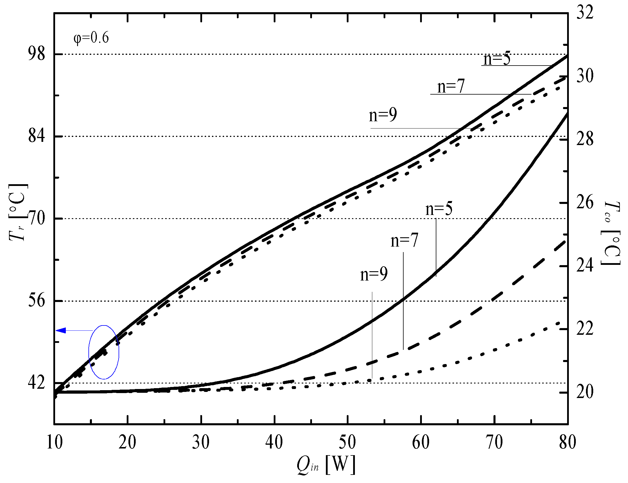
Lastly, Figure 15 illustrates variation trends concerning values of the liquid-reservoir and condenser-outlet temperature (T_r and T_co, respectively) as functions of the input thermal load (Q_in) for different values of the of the number of turns (n) comprising the condenser path. As can be seen in the figure, any increase in Q_in causes an increase in the values of both T_r and T_co. Additionally, at values of Q_in, an increase in n causes a reduction in both T_r and T_r. At Q_in = 80 W, as the value of n increases from 5 to 9, those of T_r and T_co reduce by 4.8 and 6.5 °C, respectively.

4. Conclusions

This paper reports development of a mathematical-analysis model for FLHP and CLHP via use of a nodal approach to determine temperature values at typical points within LHP. The temperature at the evaporation interface was determined using the liquid thin-film theory and kinetic theory of gases, whereas the condensation-interface temperature was determined in accordance with application of the energy-conservation principle between the two interfaces. Mathematical expressions concerning the interface temperature and condenser location were used to divide the condenser length into pure-vapor- and pure-liquid-occupied parts, by means of which liquid temperature at the condenser outlet was predicted using the ε-NTU method. Furthermore, application of the energy-conservation principle between the condenser outlet and liquid reservoir was used to determine the liquid-reservoir temperature to determine the influence of condenser-outlet temperature on the liquid reservoir.

The proposed steady-state analysis model of LHP was used to estimate the effect of various design variables on FLHP heat-transfer performance. As observed, an increase in porosity of capillary structure reduces the amount of leakage heat flowing to the liquid reservoir, thereby causing reduction in all temperatures concerning the evaporator and condenser components. It has also been demonstrated that an increase in vapor-temperature drop within the condenser causes an increase in condenser-outlet temperature, which in turn, causes an increase in liquid-reservoir temperature along with reduction overall thermal performance of the system. Furthermore, it has been demonstrated that an increase in length of the condenser path results in elevated liquid temperatures at the condenser outlet, whereas the liquid-reservoir temperature is reduced, thereby resulting in reduced temperature of the entire evaporator assembly.