Thermo-Hydro-Mechanical Coupled Modeling of Methane Hydrate-Bearing Sediments: Formulation and Application

Abstract

We present a fully coupled thermo-hydro-mechanical formulation for the simulation of sediment deformation, fluid and heat transport and fluid/solid phase transformations occurring in methane hydrate geological systems. We reformulate the governing equations of energy and mass balance of the Code_Bright simulator to incorporate hydrate as a new pore phase. The formulation also integrates the constitutive model Hydrate-CASM to capture the effect of hydrate saturation in the mechanical response of the sediment. The thermo-hydraulic capabilities of the formulation are validated against the results from a series of state-of-the-art simulators involved in the first international gas hydrate code comparison study developed by the NETL-USGS. The coupling with the mechanical formulation is investigated by modeling synthetic dissociation tests and validated by reproducing published experimental data from triaxial tests performed in hydrate-bearing sands dissociated via depressurization. Our results show that the formulation captures the dominant mass and heat transfer phenomena occurring during hydrate dissociation and reproduces the stress release and volumetric deformation associated with this process. They also show that the hydrate production method has a strong influence on sediment deformation.

1. Introduction

Methane hydrates hold vast amounts of methane gas below the sea floor and in permafrost regions [1]. If economically producible, hydrate-sourced methane could supply 10% of the global methane consumption in the coming decades [2,3,4] and bring a new level of energy self-sufficiency to countries that lack conventional reserves (e.g., Japan, India, and South Korea) [5]. Current techniques for methane production from hydrate include thermal stimulation, depressurization, and inhibitor injection [6,7], among which, depressurization is deemed the most mature approach. These techniques perturb the thermodynamic and chemical conditions of the reservoir to destabilize the hydrate phase and force its dissociation into water and gas. The release of mobile phases during dissociation and the loss of the solid hydrate phase has a significant impact in the mechanical (e.g., strength, stiffness, volumetric behavior) and hydraulic (e.g., retention curve, hydraulic conductivity) properties of the sediment and may destabilize it (e.g., [8,9]).

Over the last 20 years, several numerical models have been proposed to simulate the behavior of gas hydrate reservoirs. Initially, modeling efforts focused on evaluating the productivity of methane extraction from in situ sediments. As a result, numerous coupled thermo-hydraulic (TH) models were developed (e.g., [10,11,12,13,14,15,16,17]), which improved considerably the understanding of the TH behavior of MHBS. However, these models generally disregarded the mechanical response of the sediment or considered it with simple approaches. Numerous experimental studies have investigated the impact of hydrate dissociation on the mechanical properties of MHBS. These studies show that the sediment tends to weaken during hydrate dissociation due to a reduction of the sediment stiffness and strength with decreasing hydrate saturation (e.g., [18,19,20,21]). Additionally, they report significant changes in porosity, permeability and stress state of the sediment during dissociation (e.g., [22,23]). Field observations also note the impact of hydrate dissociation in the large-strain response of MHBS (e.g., [15,24,25,26]). Borehole instabilities, gas blowouts and seafloor subsidence have been widely reported during conventional hydrocarbon exploitation nearby hydrate reservoirs (e.g., [8,9,27]). Moreover, large underwater landslides have been related to hydrate dissociation in continental margins (e.g., [25,26,28]).

Hence, geomechanics of MHBS has recently become a key factor in reservoir simulation to ensure well-bore stability in production scenarios and mitigate hydrate-related geohazards [29]. Even though knowledge of the mechanical behavior of MHBS is still limited, current modeling efforts have focused on developing suitable constitutive laws for capturing it.

Table 1. Notable numerical solutions incorporating advanced constitutive models for MHBS.

Model Reference	Mechanical Approach
Kimoto et al. (2010) [30]	Viscoplasticity with $S_h$ dependency
Rutqvist (2011) [31]	Mohr-Coloumb elastoplasticity with $S_h$ dependency
Kim et al. (2012) [32]	Mohr-Coloumb elastoplasticity with $S_h$ dependency
Klar et al. (2013) [33]	Mohr-Coloumb elastoplasticity with $S_h$ dependency
Gupta et al. (2016) [34]	Poroelasticity with $S_h$ dependency
Sun et al. (2018) [35]	Thermodynamics-based elastoplastic model with $S_h$ dependency
Sánchez et al. (2018) [36]	Elastoplasticty with $S_h$ dependency + Damage model

lists some of the most notable thermo-hydro-mechanical (THM) formulations that incorporate advanced constitutive models for MHBS. The models listed in Table 1 consider from linear elastic to elastoplastic and visco-plastic formulations in which different dependencies of the yield function with the hydrate saturation are assumed.

Here, we develop a new fully coupled THM formulation to simulate the mechanical behavior of MHBS, particularly focusing on hydrate dissociation scenarios. The formulation builds on the established finite element simulator Code_Bright [37], which has been highly validated at solving multiphase mass and heat transport problems in the geological media (e.g., [38,39,40]) and recently applied to examine the THM behavior of MHBS [36]. We reformulate Code_Bright’s governing equations of energy and mass balance in terms of the potential porosity of the sediment (i.e., space between the mineral grains) and the remaining available porosity after the formation of hydrate and/or ice. This volumetric distinction allows isolation of the effects of mechanical deformation from the effects of hydrate and ice fluid/solid phase transformations, both affecting the hydraulic and mechanical properties of the porous medium. We also implement the elastoplastic constitutive model Hydrate-CASM [41] to capture the effect of hydrate saturation in the sediment stress-strain response, and integrate the Peng-Robinson equation of state (EoS) [42] and the thermodynamic equations proposed by [43] to compute methane gas density and solubility, respectively.

The TH capabilities of our formulation are validated against the results from a series of state-of-the-art simulators involved in the NETL-USGS first international gas hydrate code comparison study [44]. Finally, the mechanical coupling is investigated by modeling synthetic dissociation tests and validated by reproducing published experimental data from triaxial tests performed in hydrate-bearing sands dissociated via depressurization [21].

2. Methodology

This section sets the theoretical framework of the problem, develops the mathematical formulation proposed to simulate the THM behavior of MHBS and describes the strategy adopted for the numerical solution.

2.1. Components, Phases and Partial Saturations

The multicomponent and multiphase approach followed by [37] is adopted here to describe the MHBS system (Figure 1). The porous medium is considered to be composed by four mass components; mineral grains (gr), methane (m), water (w), and salt (st), that can be partitioned among five possible phases; solid (s), hydrate (h), ice (i), gas (g) and liquid (l). The incompressible mineral grains form the non-reactive solid continuum that provides the skeletal structure to the porous medium. Within the pores, hydrate and ice can grow as solid and immobile phases. Finally, fluid flow and storage are restricted to the available space between the mineral grains and hydrate and ice phases.

Similar to [45], the pore-space of the sediment is divided into two porosities (

Table 2. Volumetric relations in an elementary volume of MHBS.

Bulk volume	$V_t=V_s+V_h+V_i+V_l+V_g$
Potential void space	$V_p=V_t-V_s$
Potential porosity	${\varphi }_p=V_p/V_t$
Available void space	$V_a=V_p-V_h-V_i$
Available porosity	${\varphi }_a=V_a/V_t$
Hydrate saturation	$S_h=V_h/V_p$
Ice saturation	$S_i=V_i/(V_p-V_h$)
Gas saturation	$S_g=V_g/V_a$
Liquid saturation	$S_l=V_l/V_a$

) to isolate the effects of mechanical deformation from those related to hydrate and ice phase change on both the hydraulic and mechanical properties of the porous medium.

The potential porosity (${\varphi }_p$) is the volume of pores between the mineral grains of the sediment. This porosity is strictly related to the volumetric deformation of the sediment and is the maximum available space for the formation of hydrate and ice phases. The available porosity (${\varphi }_a$) is the volume of pores existing between solid phases (i.e., part of the potential porosity non-occupied by hydrate or ice). This porosity determines the available space for the fluids to flow or be stored, governs the sediment permeability and evolves according to variations in potential porosity and hydrate and ice phase transformations. Each phase saturation is obtained as the ratio between the its volume and the corresponding volume of voids in which it is partitioned (Table 2). Thus, the following volumetric restrictions apply:

$$S_l+S_g=1$$

(1)

and

$$\frac{{\varphi }_a}{{\varphi }_p}=(1-S_i)(1-S_h)$$

(2)

Equation (1) allows the preservation of the basic structure of the classical two-phase flow models for the gas-water system and Equation (2) provides the coupling between the gas-water system and the solid pore-filling phases.

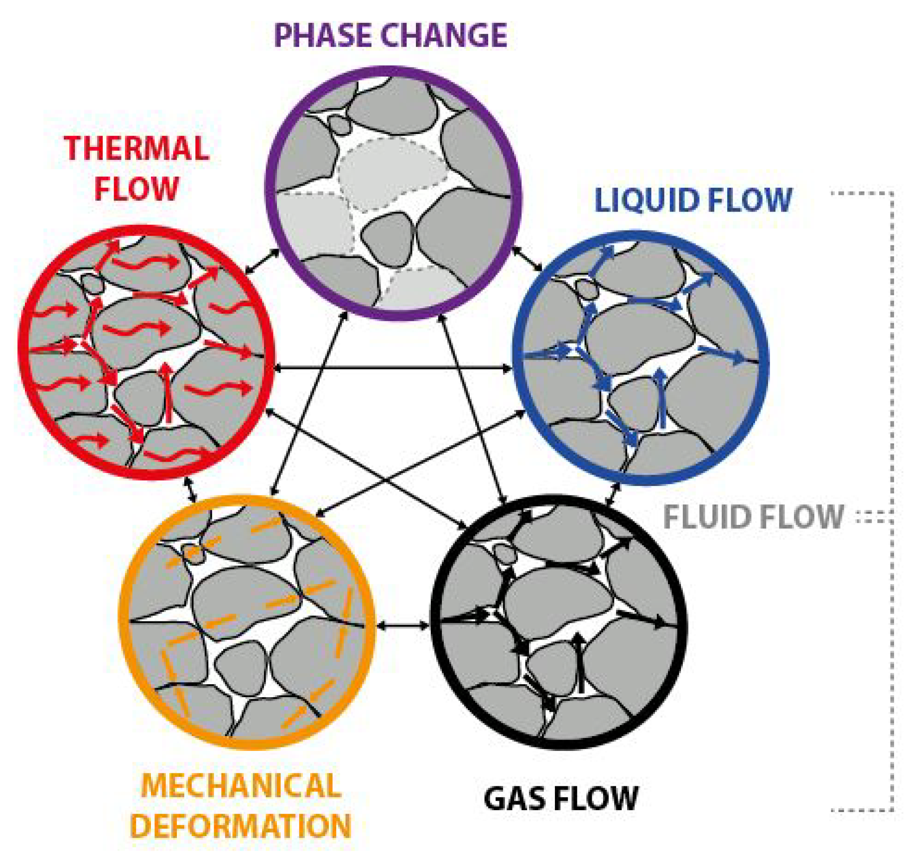
2.2. Multiphysical Coupled System

The behavior of the multiple phases considered within the pores involves four physical processes: mechanical deformation, fluid flow, thermal flow and phase change reactions (Figure 2). Each of these processes interacts with each other generating a multiphysical coupled system. Accurate representation of the interactions between these processes in the mathematical formulation is vital for adding certainty to the simulation of the mechanical behavior of MHBS.

2.3. Governing Equations

The governing equations are divided here into two main groups; (i) balance equations and (ii) constitutive equations and equilibrium constraints. All the parameters used in the formulation are listed and defined in

Table 3. Nomenclature used to define the governing equations for MHBS. Please note that superscript $\alpha$ correspond to any component of the system and subscript $\beta$ refers to the phase wherein the component is partitioned. Bold symbols denote vectors and tensors.

Roman Symbols
$a\left(T\right)$	Peng-Robinson EoS parameter	M	Slope of critical state line in p’-q space
$A_{\beta }$	Viscosity parameter	$M_{\beta }$	Molecular mass of phase $\beta$
$A\left(T\right)$	Viscosity thermal function	n	Stress-state coefficient: yield surface shape parameter
$A_h$	Hydrate surface area	$n_h$	Hydration number
$\mathbf{b}$	Body forces	$p^{\prime }$	Mean effective stress
b	Peng-Robinson EoS constant	$P_0$	Van Genuchten parameter
$B_{\beta }$	Viscosity parameter of phase $\beta$	$p_0$	Isotropic yield stress of hydrate-free sediment
$c_{\beta }^{\alpha }$	Specific heat of component $\alpha$ in phase $\beta$	$p_{0h}$	Isotropic yield stress of MHBS
$d{m}_{\beta }$	Mass change of phase $\beta$	$P_{eq}$	Hydrate phase equilibrium pressure
$D_{\beta }^{\alpha }$	Diffusion coefficient of component $\alpha$ in phase $\beta$	$P_{\beta }$	Pressure of phase $\beta$
e	Void ratio of hydrate-free sediment	$P_{{\beta }_0}$	Reference pressure for phase $\beta$
$e_{ah}$	Available void ratio of the MHBS	$P_c$	Critical pressure
$e_h$	Hydrate void ratio	$P_p$	Pore pressure
$E_{\beta }$	Energy of phase $\beta$	q	Deviatoric stress
$E_{\beta }^{\alpha }$	Energy of component $\alpha$ in phase $\beta$	${\mathbf{q}}_{\beta }$	Advective fuid flow
f	Hydrate-CASM yield function	r	Yield surface spacing ratio
$f^{\alpha }$	External mass supply of component $\alpha$	R	Subloading ratio
$f^Q$	Internal/external energy supply	$R_g$	Regnault constant
$f_w$	Peng-Robinson EoS function	$R_h$	Rate of hydrate mass change
g	Gravity forces	S	Salinity
${\mathbf{i}}_{\beta }^{\alpha }$	Diffusive flux of component $\alpha$ in phase $\beta$	$S_{\beta }$	Saturation of phase $\beta$
${\mathbf{i}}_c$	Conductive heat flow	$S_e$	Effective liquid saturation
${\mathbf{i}}_{E_{\beta }}$	Energy dispersivity in phase $\beta$	$S_{ls}$	Maximum liquid saturation
$\mathbf{I}$	Identity matrix	$S_{rl}$	Residual liquid saturation
${\mathbf{j}}_{\beta }^{\alpha }$	Mass flux of component $\alpha$ in phase $\beta$	t	Time
${\mathbf{j}}_{E_{\beta }}$	Advective flux of energy of phase $\beta$	$T_0$	Reference temperature
${\mathbf{k}}_0$	Intrinsic permeability of hydrate-free sediment	T	Temperature
$\mathbf{k}$	Intrinsic permeability of MHBS	$T_c$	Critical temperature
$k_{r_{\beta }}$	Relative permeability of phase $\beta$	$T_{eq}$	Hydrate phase equilibrium temperature
$K_{C{H}_4}$	Solubility of methane in water	$T_r$	Reduced temperature
$K_d$	Hydrate dissociation constant	$\mathbf{u}$	Displacement
$K_f$	Hydrate formation constant	u	Subloading parameter controlling the
$L_h$	Latent heat of hydrate dissociation		plastic deformations before yielding
$L_i$	Latent heat of ice melting	v	Molar volume
m	Van Genuchten parameter	V	Unitary volume
Greek Symbols
${\alpha }_B$	Biot’s coefficient	∇	Differential operator = ($\frac{\partial }{\partial x};\frac{\partial }{\partial y};\frac{\partial }{\partial z}$)
${\beta }_t$	Thermal expansion coefficient of the liquid phase	$\nu$	Poisson’s ratio
∂	Partial derivative	${\omega }_{\beta }^{\alpha }$	Mass fraction of component $\alpha$ in phase $\beta$
$|{\mathit{\epsilon }}^p|$	Norm of the incremental plastic strain	${\mu }_{\beta }$	Viscosity of phase $\beta$
${\epsilon }^v$	Volumetric strain	${\varphi }_p$	Potential porosity
${\epsilon }_{(x,y,z)}$	Cartesian strains	${\varphi }_a$	Available porosity
$\gamma$	Solute variation	${\rho }_{\beta }$	Density of phase $\beta$
$\kappa$	Slope of swelling line of hydrate-free sediment	${\rho }_{{\beta }_0}$	Reference density of phase $\beta$
${\kappa }_h$	Slope of swelling line of MHBS	$\mathit{\sigma }$	Cauchy total stress (compression positive)
${\kappa }_{rf}$	Swelling line slope reduction factor	${\mathit{\sigma }}^{\prime }$	Effective stress (compression positive)
$\lambda$	Slope of normal compression line	${\sigma }_c$	Confining stress (compression positive)
${\lambda }_c$	Composite thermal conductivity	${\theta }_{\beta }^{\alpha }$	Volumetric mass of component $\alpha$ in phase $\beta$
${\lambda }_{dry}$	Dry thermal conductivity	$\tau$	Tortuosity coefficient
${\lambda }_{sat}$	Liquid saturated thermal conductivity	$\vartheta$	Peng-Robinson acentric factor

.

(i) Balance equations

Mass balance equations

The mass balance equations are established following a compositional approach. In these equations the volumetric mass of a component in a phase (e.g., methane in the liquid phase, ${\theta }_l^m$) is the product of the mass fraction of that component (${\omega }_l^m$) and the bulk density of the phase (${\rho }_l$).

• Mass balance of mineral grains:
  The mineral grains coincide with the permanent solid phase and define the skeletal structure of the porous medium. The mass conservation of this component can be written as:

  $$\frac{\partial }{\partial t}\left({\rho }_s(1-{\varphi }_p)\right)+\nabla \left({\mathbf{j}}_s^{gr}\right)=0$$

  (3)

  where ${\mathbf{j}}_s^{gr}$ is the flux of solid and can be expressed in terms of the solid velocity ($\frac{\partial \mathbf{u}}{\partial t}$) as:

  $${\mathbf{j}}_s^{gr}={\rho }_s(1-{\varphi }_p)\frac{\partial \mathbf{u}}{\partial t}$$

  (4)
  Applying the chain rule for all the derivatives, Equation (3) can be rewritten as:

  $$(1-{\varphi }_p)\frac{\partial {\rho }_s}{\partial t}+(1-{\varphi }_p)(\frac{\partial \mathbf{u}}{\partial t}\nabla {\rho }_s)-{\rho }_s\frac{\partial {\varphi }_p}{\partial t}-{\rho }_s(\frac{\partial \mathbf{u}}{\partial t}\nabla {\varphi }_p)+{\rho }_s(1-{\varphi }_p)\nabla \frac{\partial \mathbf{u}}{\partial t}=0$$

  (5)
  Neglecting the gradients of density and porosity convected by the solid phase and under the assumption of small strain, Equation (5) can be rewritten as:

  $$\frac{\partial {\varphi }_p}{{\partial }_t}=\frac{1}{{\rho }_s}\left((1-{\varphi }_p)\frac{\partial {\rho }_s}{{\partial }_t}\right)+(1-{\varphi }_p)\nabla \frac{\partial \mathbf{u}}{\partial t}$$

  (6)

  where the term $\nabla \frac{\partial \mathbf{u}}{\partial t}$ can be expressed in the form:

  $$\nabla \frac{\partial \mathbf{u}}{\partial t}=\frac{{\partial }^2{u}_x}{\partial x\partial t}+\frac{{\partial }^2{u}_y}{\partial y\partial t}+\frac{{\partial }^2{u}_z}{\partial z\partial t}=\frac{\partial }{\partial t}({\epsilon }_x+{\epsilon }_y+{\epsilon }_z)=\frac{\partial {\epsilon }_v}{\partial t}$$

  (7)

  and ${\epsilon }_x+{\epsilon }_y+{\epsilon }_z$ are Cartesian strains.
• Mass balance of methane:
  Methane component is present in liquid, gas and hydrate phases, and its total mass balance is expressed as:

  $$\frac{\partial }{\partial t}\left(\left({\theta }_l^m{S}_l+{\theta }_g^m{S}_g\right){\varphi }_a+{\theta }_h^m{S}_h{\varphi }_p\right)+\nabla ({\mathbf{j}}_l^m+{\mathbf{j}}_g^m+{\mathbf{j}}_h^m)=f^m$$

  (8)

  where ${\theta }_l^m$, ${\theta }_g^m$ and ${\theta }_h^m$ are the volumetric mass of methane in the liquid, gas and hydrate phases, respectively. For a given temperature, pressure and salinity the term ${\theta }_l^m$ can be obtained according to [42,43], ${\theta }_g^m$ is equal to one as the gas phase is considered mono-component and ${\theta }_h^m=\frac{1}{1+n_h}$ assuming $n_h$ as 6.176.
  The mass flux terms ${\mathbf{j}}_l^m$ and ${\mathbf{j}}_g^m$ are the relative motion of methane in the liquid and gas phases, respectively, with respect to the solid phase. These terms are obtained as the sum of advective and diffusive flux terms as follows:

  $${\mathbf{j}}_l^m={\mathbf{i}}_l^m+{\theta }_l^m{\mathbf{q}}_l+{\varphi }_a{S}_l{\theta }_l^m\frac{\partial \mathbf{u}}{\partial t}$$

  (9)

  $${\mathbf{j}}_g^m={\mathbf{i}}_g^m+{\theta }_g^m{\mathbf{q}}_g+{\varphi }_a{S}_g{\theta }_g^m\frac{\partial \mathbf{u}}{\partial t}$$

  (10)
  The mass flux term ${\mathbf{j}}_h^m$ denote the relative motion of methane in the hydrate phase with respect to the solid phase as a result of the medium deformation:

  $${\mathbf{j}}_h^m={\varphi }_p{S}_h{\theta }_h^m\frac{\partial \mathbf{u}}{\partial t}$$

  (11)
  The term $f^m$ is the external sink/source of methane per unit volume. Please note that because of the compositional approach adopted in the formulation, this term do not include methane mass changes from hydrate kinetics.
• Mass balance of water:
  Water is present in liquid, ice and hydrate phases but it is neglected as vapour in the gas phase. Thus, the water total mass balance of water is expressed as:

  $$\frac{\partial }{\partial t}\left({\theta }_l^w{S}_l{\varphi }_a+\left({\theta }_i^w{S}_i(1-S_h)+{\theta }_h^w{S}_h\right){\varphi }_p\right)+\nabla ({\mathbf{j}}_l^w+{\mathbf{j}}_i^w+{\mathbf{j}}_h^w)=f^w$$

  (12)

  where ${\theta }_l^w$, ${\theta }_i^w$ and ${\theta }_h^w$ are the volumetric mass of water in the liquid, ice and hydrate phases, respectively. The term ${\theta }_l^w$ depends on the concentration of salt and methane dissolved in the liquid phase, ${\theta }_i^w$ is equal to one and ${\theta }_h^w=1-{\theta }_h^m$.
  The mass flux term of water in liquid (${\mathbf{j}}_l^w$) is computed similarly as in Equation (9), while the flux terms in hydrate (${\mathbf{j}}_h^w$) and ice phases (${\mathbf{j}}_i^w$) are computed similarly as in Equation (11) for $S_h$ and $S_i$, respectively.
  The $f^w$ is an external sink/source of water per unit volume and do not include water mass changes from hydrate kinetics.
• Mass balance of salt:
  Salt is present as a dissolved component in the liquid phase, and it is not allowed to precipitate as a solid phase. Its concentration modifies the liquid density, influences the solubility of methane and can inhibit hydrate stability conditions. The total mass balance of salt is expressed as:

  $$\frac{\partial }{\partial t}\left({\theta }_l^{st}{S}_l{\varphi }_a\right)+\nabla {\mathbf{j}}_l^{st}=f^{\mathit{st}}$$

  (13)

  where ${\theta }_l^{st}$ is the volumetric mass of salt in the liquid phase. Changes in salt concentration due to “freshening” of the pore water can be used as a tracer of ongoing hydrate dissociation and/or ice melting.
  The flux term of salt in the liquid phase (${\mathbf{j}}_l^{st}$) is the relative motion of salt in the liquid phase with respect to the solid phase and is computed similarly as in Equation (9). Finally, the term ${\mathit{f}}^{st}$ is the external sink/source term of salt.

Energy balance equation:

The equation for internal energy balance in the porous medium is established according to [37] considering the internal energy in each phase of the system, so that:

$$\begin{array}{c}\hfill \frac{\partial }{\partial t}\left((E_l{\rho }_l{S}_l+E_g{\rho }_g{S}_g){\varphi }_a+\left(E_i{\rho }_i{S}_i(1-S_h)+E_h{\rho }_h{S}_h\right){\varphi }_p\right)\\ \hfill +E_s{\rho }_s(1-{\varphi }_p)+\nabla ({\mathbf{i}}_c+{\mathbf{j}}_{E_l}+{\mathbf{j}}_{E_g}+{\mathbf{j}}_{E_i}+{\mathbf{j}}_{E_h}+{\mathbf{j}}_{E_s})=f^Q\end{array}$$

(14)

where the energy flux of fluid phases include energy dispersion, advective transport by fluid mass relative to the solid phase and that related to the soil velocity:

$${\mathbf{j}}_{E_l}={\mathbf{i}}_{E_l}+{\mathbf{j}}_l^m{E}_l^m+{\mathbf{j}}_l^w{E}_l^w+{\mathbf{j}}_l^{st}{E}_l^{st}+E_l{\rho }_l{\varphi }_a{S}_l\frac{\partial \mathbf{u}}{\partial t}$$

(15)

$${\mathbf{j}}_{E_g}={\mathbf{i}}_{E_g}+{\mathbf{j}}_g^m{E}_g+E_g{\rho }_g{\varphi }_a{S}_g\frac{\partial \mathbf{u}}{\partial t}$$

(16)

with

$$E_l{\rho }_l={\theta }_l^m{E}_l^m+{\theta }_l^w{E}_l^w+{\theta }_l^{st}{E}_l^{st}$$

(17)

Please note that $E_l^m$ and the dispersive terms (${\mathbf{i}}_{E_l}$ and ${\mathbf{i}}_{E_g}$) have been neglected in our simulations.

The energy flux of solid phases only depend on the advective transport related to the soil velocity, so that:

$${\mathbf{j}}_{E_h}=E_h{\rho }_h{\varphi }_p{S}_h\frac{\partial \mathbf{u}}{\partial t}$$

(18)

$${\mathbf{j}}_{E_i}=E_i{\rho }_i{\varphi }_p(1-S_h)S_i\frac{\partial \mathbf{u}}{\partial t}$$

(19)

$${\mathbf{j}}_{E_s}=E_s{\rho }_s(1-{\varphi }_p)\frac{\partial \mathbf{u}}{\partial t}$$

(20)

For which exothermic/endothermic changes caused by hydrate formation/dissociation and ice formation/melting are considered through the latent heat of each phase transformation (

Table 4. Specific energy expression and representative values of specific and latent heat for each phase of the system.

Phase	Specific Energy	Specific and Latent Heat
Gas (g)	$E_g=c_g(T-T_0)$	$c_g$ = 2500 J (Kg K)−1
Hydrate (h)	$E_h=L_h+c_h(T-T_0)$	$c_h$ = 2108 J (Kg K)−1; †$L_h$ = 3.39 e5 J Kg−1
Ice (i)	$E_i=L_i+c_i(T-T_0)$	$c_i$ = 3144 J (Kg K)−1; †$L_i$ = 3.34 e5 J Kg−1
Liquid (l)	$E_l^w=c_l^w(T-T_0)$	$c_l^w$= 4184 J (Kg K)−1
	$E_l^{st}=1.42e^5$ + $c_l^{st}(T-T_0)$	$c_l^{st}$ = 2200 J (Kg K)−1
Solid (s)	$E_s=c_s(T-T_0)$	$c_s$ = 874 J (Kg K)−1

^†$L_h$ and $L_i$ are positive for hydrate dissociation and ice melting respectively.

) and the term $f^Q$ is the external supply of energy per unit volume.

Momentum balance equation:

The momentum balance equation for the bulk porous medium reduces to the equilibrium of total stresses if the inertial terms are neglected:

$$\nabla \mathit{\sigma }+\mathbf{b}=0$$

(21)

Equation (21) is formulated based on the infinitesimal strain theory, uses an additive decomposition of the total strain tensor and assumes a Biot’s coefficient ${\alpha }_B$ = 1 for the fluid-solid coupling (

Table 5. Constitutive equations for MHBS system and dependent variables computed using each constitutive law. Please note that values for the parameters used in the TH simulation are also given.

Constitutive Law	Equation	Dependent Variable
Advective fluid flow
Darcy’s law	${\mathbf{q}}_{\beta }=-\frac{\mathbf{k}{k}_{r_{\beta }}}{{\mu }_{\beta }}(\nabla P_{\beta }-{\rho }_{\beta }\mathbf{g})\beta =l,g$	Advective fluid flow, ${\mathbf{q}}_l$ and ${\mathbf{q}}_g$
Kozeny’s model	$\mathbf{k}={\mathbf{k}}_0\frac{{\varphi }_a^3}{{(1-{\varphi }_a)}^2}\frac{{(1-{\varphi }_p)}^2}{{\varphi }_p^3}$
	${\mathbf{k}}_0=1$ × ${10}^{-13}$ m2
	$k_{r_l}=\sqrt{S_e}{\left(1-{(1-S_e^{1/m})}^m\right)}^2$
	$k_{r_g}=1-k_{r_l}$
	$m^{‡}=0.645$
	${\mu }_{\beta }=A_{\beta }$exp$\left(\frac{B_{\beta }}{273.15+T}\right)$
	$A_l=2.1$ × ${10}^{-12}$ MPa s; $B_l$ = 1808.5 K
	$A_g=1.48$ × ${10}^{-12}$ MPa s; $B_g$ = 119.4 K
Retention curve [46]	$S_e=\frac{S_l-S_{rl}}{S_{ls}-S_{rl}}={\left(1+{\frac{P_g-P_l}{P_0}}^{\frac{1}{1-m}}\right)}^{-m}$	Saturation of mobile phases, $S_l$ and $S_g$
	$P_0^{‡}=0.075$ MPa
Liquid density [37]	${\rho }_l={\rho }_{l_0}\left(1+{\beta }_t(P_l-P_{l_0})+A\left(T\right)+\gamma {\omega }_l^{st}\right)$	Liquid density, ${\rho }_l$
	$A\left(T\right)=\frac{(T+288.9414){(T-3.9863)}^2}{50,8929.2(T+68.12963)}$
	${\rho }_{l_0}$ = 1002.6 kg/m3
	${\beta }_t=4.5\times {10}^{-4}$ MPa−1
	$P_{l_0}=0.1$ MPa
	$\gamma =0.6923$
	${\omega }_l^{st}=0$
Gas density [42]	$P_g=\frac{R_{g}T}{v-b}-\frac{a\left(T\right)}{v(v+b)+b(v-b)}$	Gas density, ${\rho }_g$
	$a\left(T\right)=0.45724R_g^2{T}_c^2/P_c{[1+f_w(1-T_r^{0.5})]}^2$
	$f_w=0.37464+1.54226\vartheta -0.26992{\vartheta }^2$
	$\vartheta =0.0015$
	$b=0.0778R{T}_c/P_c$
	$R_g=8.3144598$ J/mol K
	$P_c=4.60$ MPa
	$T_r=T/T_c,T_c=190.4$ K
	${\rho }_g=\frac{M_g{P}_g}{R_{g}T}$
	$M_g=0.016042$ Kg/mol
Non-advective fluid flow
Fick’s law	${\mathbf{i}}_{\beta }^{\alpha }={\varphi }_a\tau {\rho }_l{S}_l{D}_l^{\alpha }\mathbf{I}\nabla {\omega }_l^{\alpha }\alpha =m,st$	Diffusive flux, ${\mathbf{i}}_l^m$ and ${\mathbf{i}}_l^{st}$
	$D_l^m=5.9\times {10}^{-6}$ exp$\left(\frac{{(273.15+T)}^{2.3}}{P_g}\right)$
	$D_l^{st}=1.1\times {10}^{-4}$ exp$\left(\frac{-24530}{R_g(273.15+T)}\right)$
	$\tau =1$
Fourier’s law	${\mathbf{i}}_c=-{\lambda }_c\nabla T$	Conductive heat flow, ${\mathbf{i}}_c$
	†${\lambda }_c={\lambda }_{sat}\sqrt{S_l}+{\lambda }_{dry}(1-\sqrt{S_l})$
	${\lambda }_{sat}=2$ W/mK, ${\lambda }_{dry}=2.18$ W/mK
Stress-strain behavior
Effective stress [47]	${\mathit{\sigma }}^{\prime }=\mathit{\sigma }-{\alpha }_B{P}_p\mathbf{I}$	Effective stress tensor, ${\mathit{\sigma }}^{\prime }$
	${\alpha }_B=1$
Hydrate-CASM [41]	Subloading yield function	Stress tensor, $\mathit{\sigma }$
	$f={\left(\frac{q}{M{p}^{\prime }}\right)}^n+\frac{1}{ln\left(r\right)}ln\left(\frac{p^{\prime }}{R{p}_{0h}^{\prime }}\right)$
	$dR=-ulnR|d{\mathit{\epsilon }}^p|$
	Densification mechanism
	$e_{ah}=e-e_h;e_h=e(S_h+S_i)$
	${\kappa }_h=\kappa {\kappa }_{rf}$
	${\kappa }_{rf}$ = 0 if $(S_h+S_i)=0$
	${\kappa }_{rf}=3{(S_h+(1-S_h)S_i)}^2-2.68(S_h+(S_h+(1-S_h)S_i)+0.9934$
	if $0<(S_h+(1-S_h)S_i)\le 0.42$
	$p_{0h}^{\prime }=e^{\frac{e(S_h+S_i)}{\lambda -{\kappa }_h}}{p^{\prime }}_0^{\frac{\lambda -\kappa }{\lambda -{\kappa }_h}}$

^†${\lambda }_c$ is not computed in terms of $S_h$ or $S_i$. This simplification valid for low saturations of ice [48]; ^‡ m and ^‡ $P_0$ values correspond to those given in the benchmark problem analyzed in Section 3.1. [44]. The m value is included within the range of values reported in the literature for gas hydrate numerical simulation studies (e.g., [49,50]); Please note that $e_{ah},{\kappa }_h$ and $p_{0h}^{\prime }$ recover the hydrate-free parameters $e,\kappa$ and $p_0^{\prime }$ when $(S_h+S_i)$ = 0; The use of bold symbols denote vectors and tensors.

).

The constitutive equations for MHBS allow rewriting Equation (21) in terms of the solid velocities, gas and fluid pressure and temperature.

(ii) Constitutive equations and equilibrium constraints

A set of constitutive laws and equilibrium restrictions are used in the formulation to establish the link between the primary (i.e., solid displacements, $\mathbf{u}$; liquid pressure, $P_l$; gas pressure, $P_g$; temperature, T and salinity, S) and the dependent variables of the system (listed in Table 5 and

Table 6. Equilibrium restrictions for MHBS system. The dependent variables computed using each of the equilibrium restrictions are also included.

Equilibrium Restriction	Equation	Dependent Variable
Hydrate phase change
Hydrate phase boundary [43]	$ln\left(P_{eq}\right)=-1.644866$ × ${10}^3-0.1374178T+5.4979866$ × ${10}^4/T+2.64118188$ × ${10}^{2}ln\left(T\right)+S(1.1178266$ × ${10}^4+7.67420344T-4.515213$ × ${10}^{-3}{T}^2-2.04872879$ × ${10}^5/T-2.17246046$ × ${10}^{3}ln\left(T\right))+S^2(1.70484431$ × ${10}^2+0.118594073T-7.0581304$ × ${10}^{-5}{T}^2-3.0979619$ × ${10}^3/T-33.2031996ln\left(T\right))$	Equilibrium pressure, $P_{eq}$
Methane solubility	$ln{\left(K_{C{H}_4}\right)}_{P_g}=ln{\left(K_{C{H}_4}\right)}_{P_{eq}}\frac{ln{\left(K_{C{H}_4}\right)}_{0.1MPa}}{ln{\left(K_{C{H}_4}\right)}_{T_{eq}\left(P_g\right)}}$	Dissolved methane concentration, ${\omega }_l^m$
[43]	$ln{\left(K_{C{H}_4}\right)}_{P_{eq}}=-2.5640213$ × ${10}^5-1.644805$ × ${10}^{2}T+9.1089042$ × ${10}^{-2}{T}^2+4.90352929$ × ${10}^6/T+4.93009113$ × ${10}^{4}ln\left(T\right)+S[-5.1628513$ × ${10}^2-0.33622376T+1.8819904$ × ${10}^{-4}{T}^2+9.76525718$ × ${10}^3/T+99.523354ln\left(T\right)]$
[51]	$ln{\left(K_{C{H}_4}\right)}_{0.1MPa}=1$ × ${10}^{-9}\left[-417.5053+599.8626(100/T)+380.3636ln(T/100)-62.0764T/100+S[-0.06423+0.03498(T/100)-0.0052732{(T/100)}^2]\right]$
	$ln{\left(K_{C{H}_4}\right)}_{T_{eq}\left(P_g\right)}=1$ × ${10}^{-9}\left[-417.5053+599.8626(100/T_{eq}\left(P_g\right))+380.3636ln(T_{eq}\left(P_g\right)/100)-62.0764T_{eq}\left(P_g\right)/100+S[-0.06423+0.03498(T_{eq}\left(P_g\right)/100)-0.0052732{(T_{eq}\left(P_g\right)/100)}^2\right]$
	${\omega }_l^m=1.604$ × ${10}^{-2}{K_{C{H}_4}}_{P_g}Kg/Kg$
Hydrate kinetic rate [52,53]	$R_h(T,P_g)={\varphi }_p{S}_h{A}_h\left(K_d\langle P_{eq}\left(T\right)-P_g\rangle -K_f\langle P_g-P_{eq}\left(T\right)\rangle \right)$	Hydrate mass change, $d{m}_h$
	$A_h=0.375\mu /m$
	$K_d=124\times {10}^3$exp$(-9400/T\left(K\right))mol/m^{2}Pas$
	$K_f=0.5875\times {10}^{-11}mol/m^{2}Pas$
	†$d{m}_h=M_h{R}_h(T,P_g)$
	$M_h=0.018016n_h+0.016042Kg/mol$
Ice phase change
Freezing characteristic function [54]	$1{-}^{†}{S}_i=\left(1+{\left(\frac{1-(1-{\rho }_i/{\rho }_l)P_l-{\rho }_i{L}_{i}ln(T/273.15)}{P_0}\right)}^{\frac{1}{1-m}}\right){)}^{-m}$	Ice saturation, $S_i$
	${\rho }_i=0.91·{\rho }_l$

^† See Appendix A for the derivation of hydrate and ice mass conservation equations.

). These equations allow capturing the coupling among the various physical phenomena considered in the system and close the mathematical formulation.

Stress - strain behavior of MHBS

Several experimental studies show that MHBS have a greater stiffness, strength, dilation, and softening behaviors with increasing hydrate saturation (e.g., [55,56,57,58,59,60,61]). The increase in sediment strength due to hydrate has been widely attributed to a physical bonding between the hydrate crystals and the sediment grains. This bonding has been modeled using different strategies; (i) addition of a cohesion constituent in the failure criteria [60,62,63,64], (ii) enlargment of the yield surface by cohesion and dilation [65,66], (iii) partition of the stress between hydrate and matrix in a bonding damage framework [65,67], (iv) attribution of physical bonding properties in discrete element methods (DEM) [68] and (v) expansion of the failure envelope in a spatially mobilized plane (SMP) model [69]. Refs. [70,71] propose that kinematics might govern the increase in strength observed in hydrate-bearing sands. Alternatively, [41] propose that the greater strength and dilatancy observed in MHBS can be explained by densification and stiffening of the host sediment due to pore invasion by hydrate.

The constitutive model Hydrate-CASM [41] is integrated in our formulation to predict the mechanical response of MHBS. This elastoplastic model extends the formulation of the CASM model [72] by implementing the subloading surface model [73] and the densification mechanism. The densification is a novel mechanism for MHBS that attributes hydrate-related changes in the void ratio, the swelling line slope and the volumetric yield stress of the sediment to stress-strain changes (Table 5). The performance of the Hydrate-CASM model has been tested over a range of hydrate saturations and confining stress using experimental data from triaxial tests performed in synthetic hydrate-bearing sands and validated against the outputs from other notable constitutive models for MHBS that simulated the same experimental data (Figure 3).

Hydrate and ice phase boundaries

The dominant parameters governing the stability field of methane hydrates in marine sediments are pressure, temperature and salinity. Our formulation employs the empirical solution proposed by [43] to define the P-T conditions that describe the equilibrium of methane hydrates in saline water (Figure 4). Above the hydrate phase equilibrium curve (i.e., $P_g>P_{eq}$, shaded area in Figure 4), hydrate can form when the concentration of methane dissolved in the liquid phase is at or above saturation value [75]. Our formulation computes methane solubility at dissociation pressure as a function of salinity and temperature following the empirical proposal of [43] (Table 6). This function is combined with the IUPAC recommendation at $P_g$ = 0.1 MPa [51] to extend the calculation of methane solubility in water at any other given pressure (Table 6). The resulting estimation of methane concentration in water (${\omega }_l^m$) is key to model the upward transport of gas by means of diffusion and advection. It can also be used to predict the resulting shape of sulfate profiles in pore water (e.g., [76,77]) and the volume and distribution of hydrate formations in marine sediments (e.g., [78]).

At P-T conditions below the hydrate phase equilibrium curve (i.e., $P_g<P_{eq}$, white area in Figure 4), hydrate dissociates into its forming components. Our formulation assumes hydrate phase change to be governed by first order kinetics as suggested by [52,53], in which the rate of phase change is proportional to the product of the hydrate surface area and the driving force (i.e., pressure difference between the phase equilibrium and gas pore pressure) (Table 6).

Water-to-ice transformation may also take place in MHBS during temperature dropping if hydrate formation is restricted by insufficient methane gas, or due to endothermic cooling at fast depressurization. Ice changes are computed using the freezing characteristic function proposed by [54] (Table 6). This function is derived from the thermodynamic equilibrium between liquid and ice phases in pores in frozen soils and employs van Genuchten’s (1980) model to relate the degree of unfrozen water saturation to the thermodynamic properties of the sediment. As stated in Table 5 our formulation consider changes in ice saturation to have the same mechanical effects that hydrate phase change.

2.4. Numerical Solution Strategy

The PDE’s (Partial Differential Equations) system presented is solved numerically following the procedure established in [37]. The Galerkin finite element method (FEM) is adopted for the spatial discretization, while finite differences are used for the temporal discretization via an implicit scheme (backward Euler method) that incorporates an automatic sub-stepping procedure based on error control [79]. Also, a mass conservative approach is adopted by directly discretizing the storage terms [80,81], and the mechanical problem is solved using an implicit stress point algorithm (SPA) [82].

Once the formulation is discretized, this can be represented as a system of algebraic equations that are linearized via the Newton-Raphson scheme. Then, LU decomposition and back-substitution (non-symmetric matrix) or conjugate squared gradients are used to solve the system of equations simultaneously (monolithic solution) in a fully coupled manner.

3. Results and Discussion

3.1. Thermo-Hydraulic Validation

In this section, we reproduce the benchmark problem P2 proposed in the NETL-USGS first international gas hydrate code comparison study. The initial problem conditions, model parameters and further specifications can be found in https://www.netl.doe.gov/node/7285. Problem P2 analyzes a 20 m one-dimensional horizontal closed domain (no flow boundary conditions) initialized with gradients in liquid and gas pressure, and temperature that yield aqueous saturated conditions on half of the domain and aqueous unsaturated conditions on the other half (Figure 5a). We have simulated the problem in two-dimensions and have used a non-uniform mesh, with a higher concentration of elements in the contact between the two domains, to represent better the problem solution.

The initial conditions of the problem P2 are designed to trigger complete dissociation of the hydrate phase via the thermal capacitance of the right half of the domain. From these conditions, the simulation proceeds to reach the equilibrium in temperature and pressure along the domain. During the transition, the hydrate begins to dissociate at the contact between both domains and the dissociation front (vertical dotted line Figure 5e) advances progressively to the left. After 10 days of simulation hydrate dissociation occurs simultaneously with hydrate reformation. As shown in Figure 5e, hydrate saturation at 100 and 1.000 days of simulation increases with respect to the previous value as we move away from the dissociation front towards the left side. The low temperature in this side of the domain in combination with the endothermic nature of the dissociation reaction and the increase in pore pressure due to the migration of free gas allows reaching the P-T conditions for hydrate reformation.

The good matching observed between our results and those from the simulators involved in the code comparison study (i.e., HydResSim, MH-21, CMG STARS, STOMP-HYD, TOUGH-FX and Univ-Houston) allows validating the capacity of our formulation at capturing the dominant mass and heat transfer phenomena during gas hydrate dissociation.

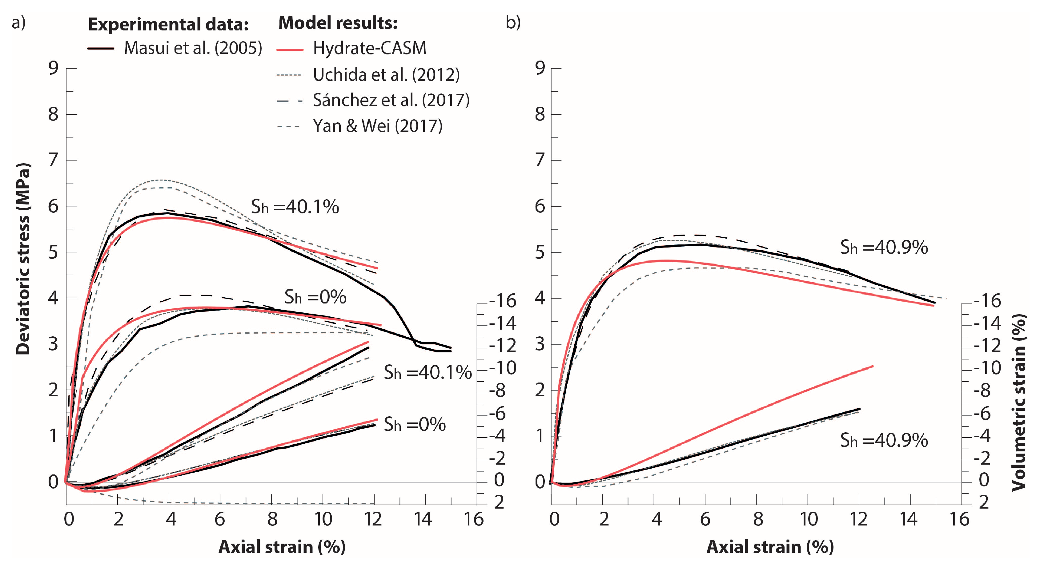
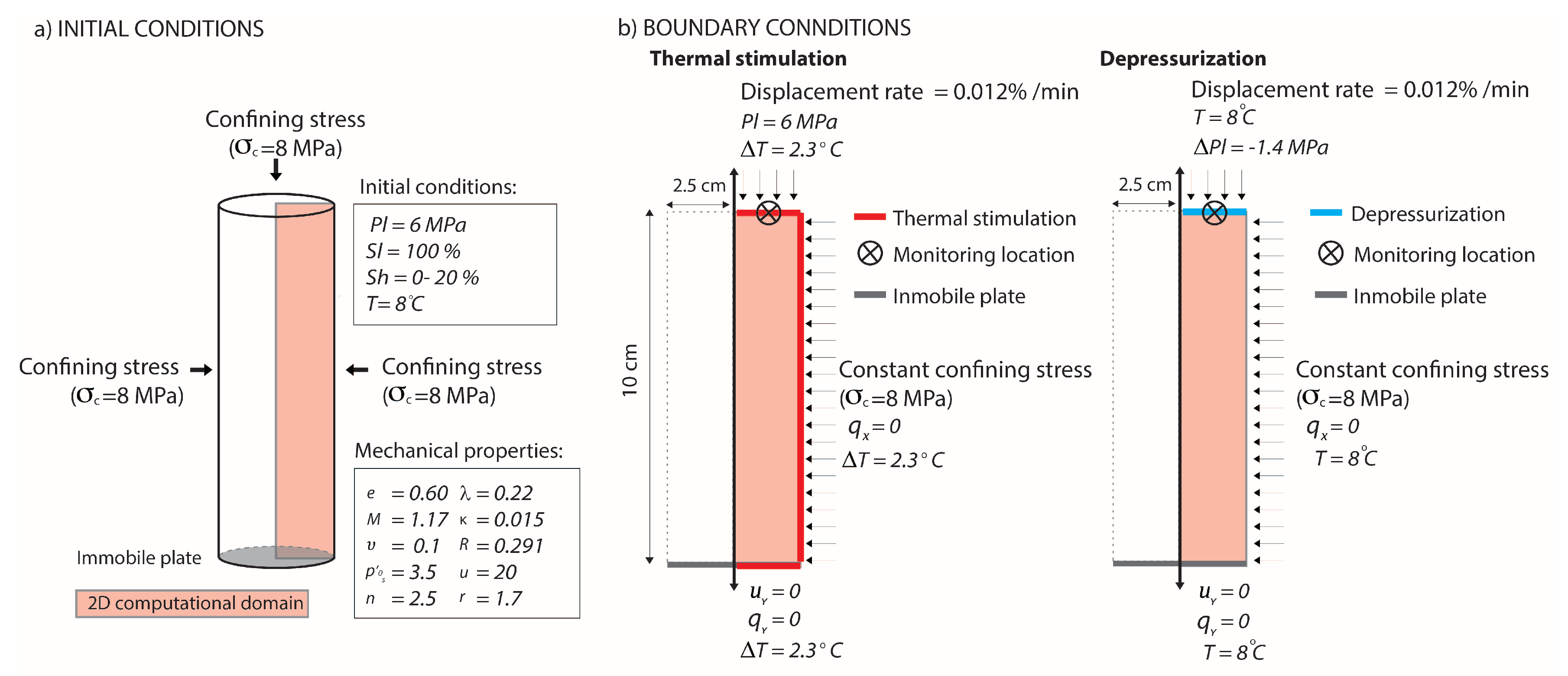
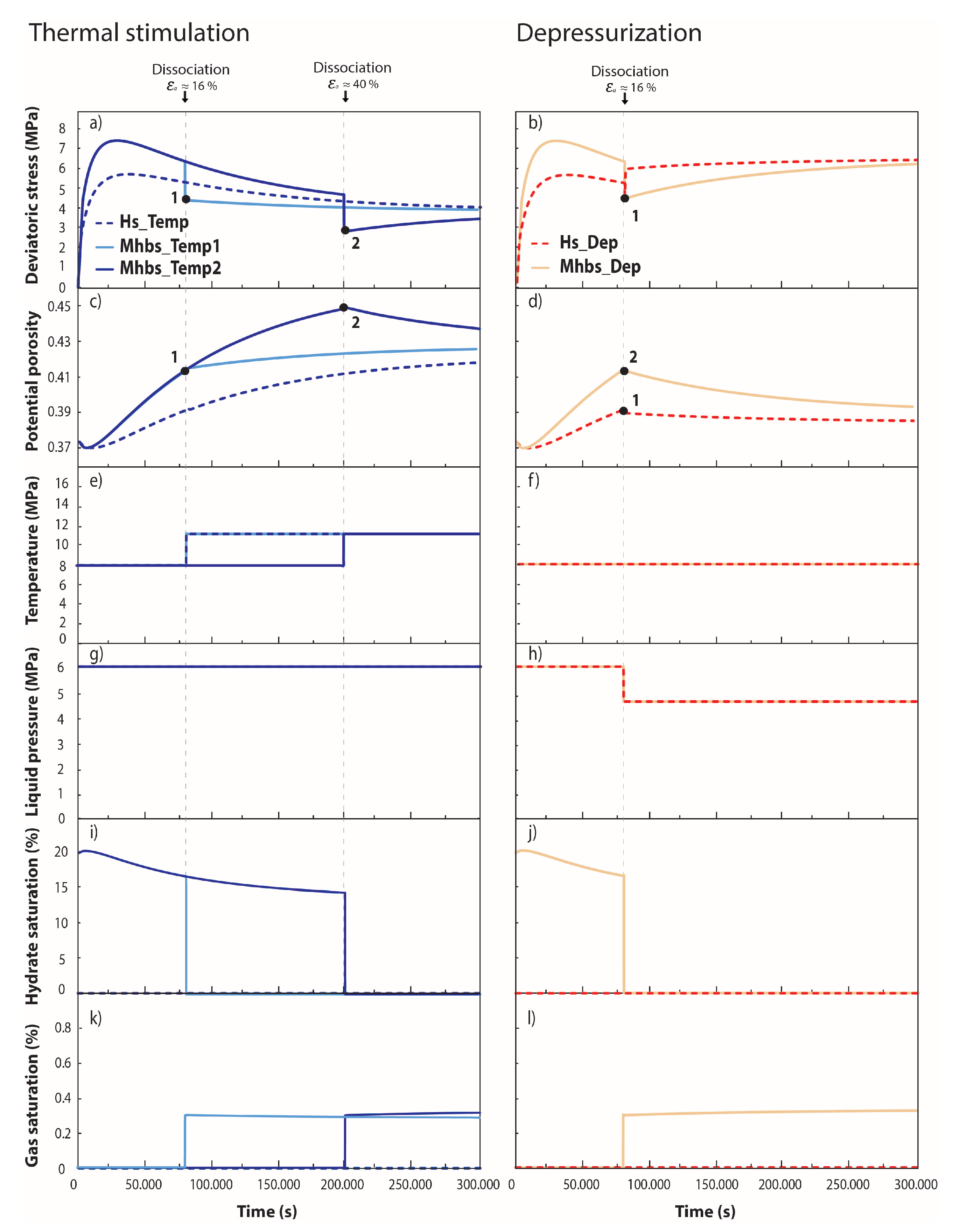
3.2. THM Modelling of Synthetic Experimental Tests

In this section, various synthetic triaxial tests are simulated to investigate the stress-strain and volumetric deformation characteristics of MHBS during hydrate dissociation under strain controlled shear. For the simulations, we assume two-dimensional axisymmetric jacketed sand specimens of 10 cm × 5 cm, of which a radial plane of 10 cm × 2.5 cm is used as computational domain (shaded area in Figure 6). The right-hand side of the domain has a boundary condition of constant total stress and the bottom is immobile. All the simulations are conducted under constant compression rate of 0.012%/min with drained conditions only at the top of the sample. The particular conditions employed in each simulation are listed in

Table 7. Test conditions adopted in the simulations.

Test Conditions
Test Name	Temperature (°C)	Confining Pressure (MPa)	Liquid Pressure (MPa)	Hydrate Saturation (%)	Remarks
Hs_Temp	8 → 11.3	8	6	0	Thermal stimulation at ${\epsilon }_a=16\%$
Mhbs_Temp1	8 → 11.3	8	6	20	Thermal stimulation at ${\epsilon }_a=16\%$
Mhbs_Temp2	8 → 11.3	8	6	20	Thermal stimulation at ${\epsilon }_a=40\%$
Hs_Dep	8	8	6 → 4.6	0	Depressurization at ${\epsilon }_a=16\%$
Mhbs_Dep	8	8	6 → 4.6	20	Depressurization at ${\epsilon }_a=16\%$

.

We label as Hs_Temp and Hs_Dep the two simulations used to characterize the mechanical response of the host sediment specimen ($S_h=0\%$) subjected to thermal stimulation (8 → 11.3 °C) and depressurization (6 → 4.6 MPa). These simulations provide a reference behavior that allows distinguishing the mechanical effects of temperature and pressure variations from those related to hydrate dissociation in MHBS. For the dissociation tests, MHBS specimens ($S_h\ne 0\%$) are sheared up to an axial strain of approximately 16% (Mhbs_Temp1, Mhbs_Dep) and 40% (Mhbs_Temp2). Then, depressurization and/or thermal stimulation are imposed over a period of 100 seconds and the final liquid pressure (4.6 MPa) and temperature (11.3 °C) are kept constant thereafter.

Figure 7 shows the simulated evolution of the deviatoric stress, potential porosity, temperature, liquid pressure and hydrate and gas saturation during the complete triaxial loading history for each simulation.

The host specimen Hs_Temp, sheared under constant pore pressure and subjected to thermal stimulation, is characterized by a peak in the deviatoric stress followed by softening (Figure 7a) and dilatant response (Figure 7c). The specimens with hydrate (Mhbs_Temp1 and Mhbs_Temp2) show a greater peak in the deviatoric stress and a more dilatant response than the corresponding host sediment before dissociation is simulated. Then, dissociation via thermal stimulation leads to a drop in the deviatoric stress (points 1 and 2 in Figure 7a) as well as to a reduction in the dilatant response (point 1 in Figure 7c) or a compressive behavior of the dissociated sediment (point 2 in Figure 7c).

The mechanical behavior of the host specimen Hs_Dep subjected to depressurization is highly influenced by the increase in effective confining stress associated with it. Depressurization leads the host sediment to shift from a softening to a hardening response and from a dilatant to a compressive volumetric behavior (point 1 in Figure 7b,d). For the hydrate-bearing specimen Mhbs_Dep, the effects on the effective stress induced by depressurization adds to the mechanical effect of hydrate dissociation. Upon dissociation specimen Mhbs_Dep starts contracting under shear (point 2 in Figure 7d) rather than reducing its dilatant behavior, as observed in the equivalent specimen subjected to thermal stimulation (point 1 in Figure 7c).

These results capture two important features of the mechanical response of MHBS during hydrate dissociation under strain controlled shear. Hydrate dissociation leads to a drop of the deviatoric stress which is associated with the shrinking of the yield surface due to sediment mechanical weakening [41]. In consequence, the sediment shows a less dilatant behavior than the corresponding host sediment or even a contractant response under shear. Our results also show that the volumetric deformation of the sediment after dissociation strongly depends on the hydrate production method. Point 2 in Figure 7d clearly shows that dissociation via depressurization leads the specimen contraction while dissociation by thermal stimulation does not (point 1 in Figure 7c).

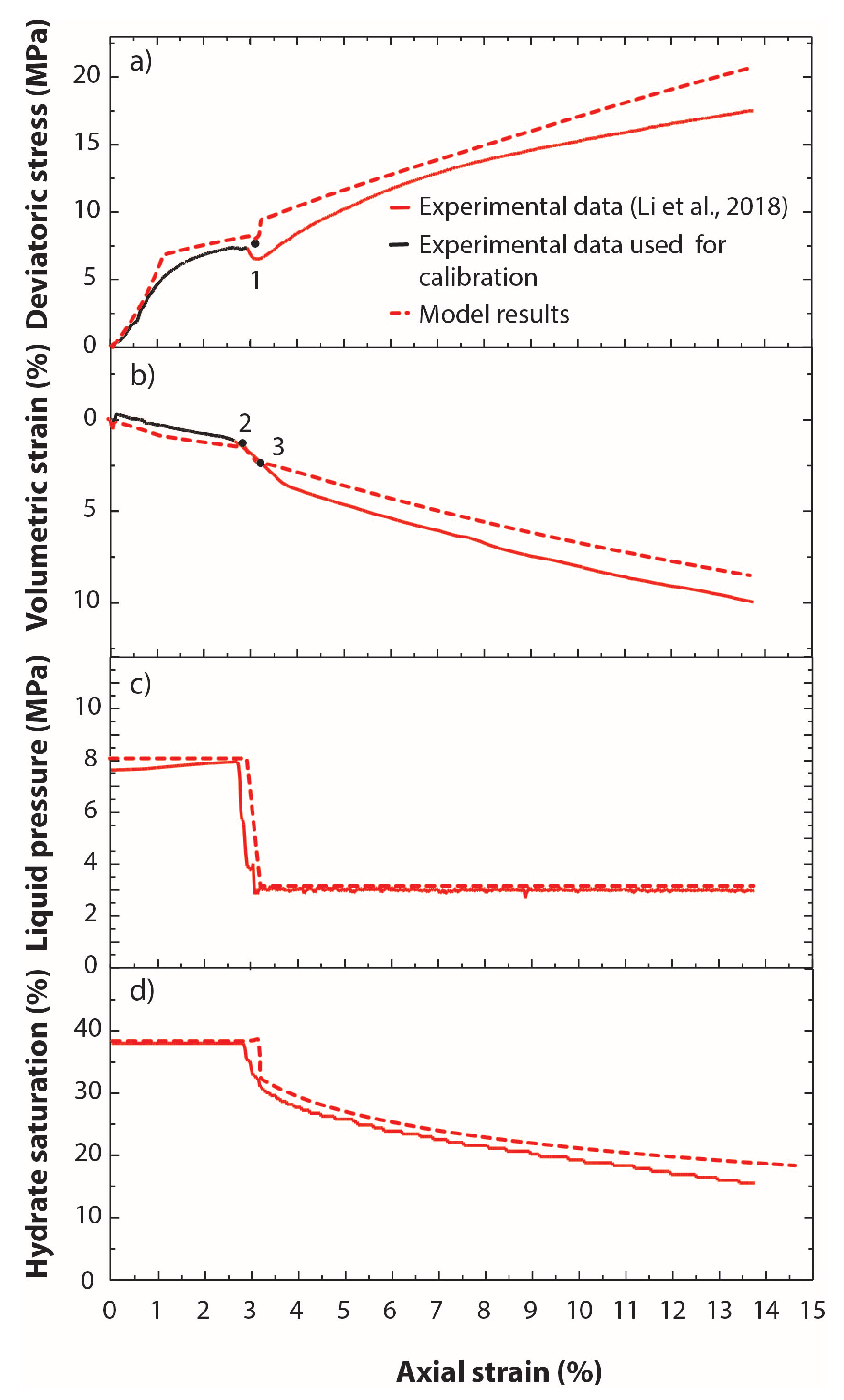
3.3. THM Modelling of the Experimental Tests of Li et al. (2018)

The multistage triaxial shear test conducted by [21] is used in this section to examine the capabilities of our formulation at capturing the effect of hydrate dissociation via depressurization in the mechanical response of synthetic MHBS. Figure 8 summarizes the mechanical properties and the initial and boundary conditions considered in the simulation. The modeling is approached here in two steps, firstly the mechanical behavior of the specimen with a constant hydrate saturation of 38.5% is calibrated based on the experimental deviatoric stress-axial strain and volumetric strain-axial strain relationships obtained before depressurization is applied (black solid lines in Figure 9a,b). Once the mechanical properties are calibrated, hydrate dissociation is simulated at approximately 2.5% of axial strain by depressurizing the specimen from a liquid pressure of 8 MPa to 3 MPa. The depressurization is applied as a boundary condition on top of the specimen (blue line in Figure 8) while this is subjected to a constant triaxial compression rate of 0.2%/min. Temperature is imposed on the top, base and right-hand side of the computational domain to simulate the circulation of fluid at a constant temperature around the specimen.

Results in Figure 9 show that once depressurization is induced, our formulation captures a subtle drop in the deviatoric stress (point 1 in Figure 9a) as well as an increase in volumetric strain (points 2 to 3 in Figure 9b). However, the model overestimates the maximum deviatoric stress after dissociation and slightly underestimates the volumetric strain at the end of the triaxial. For comparison purposes, the evolution of hydrate saturation with the axial strain is plotted removing the change in $S_h$ due to sediment deformation (i.e., changes in hydrate saturation are related only to the chemical reaction). Figure 9d shows that the model captures the rate of hydrate dissociation.

4. Conclusions

Hydrate dissociation has a significant effect on the THM properties of MHBS and may cause its mechanical destabilization. Our formulation captures the mass and heat transfer phenomena during hydrate dissociation in the porous medium. Particularly, the TH performance shows that the migration of the dissociation front caused by thermal stimulation and depressurization and the volume of hydrate that reforms due to gas migration are closely reproduced. Regarding the coupling with the mechanical formulation, our synthetic results show that dissociation leads to a drop in the deviatoric stress and to a less dilatant or even contracting behavior of the dissociated MHBS in comparison to the host sediment. Particularly, it is observed that sediment may contract in cases when the deviatoric stress drops below the failure envelope of the host sediment. Our synthetic results also suggest that the deformation of MHBS strongly depends on the hydrate production method. They show that specimens subjected to hydrate dissociation via depressurization are more likely to show contractant behavior under shear than those subjected to thermal stimulation because of the increase in effective stress. We finally illustrate that our formulation successfully reproduces the main THM features observed in dissociation tests performed in real specimens.

References

1. Milkov, A.V. Global estimates of hydrate bound gas in marine sediments: How much is really out there? Earth Sci. Rev. 2004, 66, 183–197. [Google Scholar] [CrossRef]
2. Krey, V.; Canadell, J.G.; Nakicenovic, N.; Abe, Y.; Andruleit, H.; Archer, D.; Grubler, A.; Hamilton, N.T.M.; Johnson, A.; Kostov, V.; et al. Gas hydrates: Entrance to a methane age or climate threat? Environ. Res. Lett. 2009, 4, 34007. [Google Scholar] [CrossRef]
3. Muradov, N. Decarbonization at crossroads: The cessation of the positive historical trend or a temporary detour? Energy Environ. Sci. 2013, 6, 1060–1073. [Google Scholar] [CrossRef]
4. Smith, C.A. Energy Resource Potential of Methane Hydrate: An Introduction to the Science and Energy Potential of a Unique Resource. 2011. Available online: www.netl.doe.gov (accessed on 23 May 2019).
5. Birchwood, R.; Dai, J.; Shelander, D.; Boswell, R.; Collett, T.; Cook, A.; Dallimore, S.; Fujii, K.; Imasato, Y.; Fukuhara, M.; et al. Developments in gas hydrates. Oilfield Rev. 2010, 22, 18–33. [Google Scholar]
6. Collett, T.S.; Johnson, A.H.; Knapp, C.C.; Boswell, R. Natural gas hydrates—Energy resource potential and associated geologic hazards. AAPG Mem. 2009, 89, 146–219. [Google Scholar]
7. Ruppel, C.D. Gas hydrate in nature. U.S. Geol. Surv. Fact Sheet 2018, 2017–3080, 4. [Google Scholar]
8. Hovland, M.; Gudmestad, O.T. Potential influence of gas hydrates on seabed installations. In Natural Gas Hydrates; Paull, C.K., Dillon, W.P., Eds.; Geophysical Monograph Series; American Geophysical Union: Washington, DC, USA, 2001; Volume 124, pp. 307–315. [Google Scholar]
9. Nagel, N. Compaction and subsidence issues within the petroleum industry: From Wilmington to Ekofisk and beyond. Phys. Chem. Earth Part A Solid Earth Geod. 2001, 26, 3–14. [Google Scholar] [CrossRef]
10. Ahmadi, G.; Ji, C.; Smith, D.H. Numerical solution for natural gas production from methane hydrate dissociation. J. Petroleum Sci. Eng. 2004, 41, 269–285. [Google Scholar] [CrossRef]
11. Kurihara, M.; Ouchi, H.; Inoue, T.; Yonezawa, T.; Masuda, Y.; Dallimore, S.R.; Collett, T.S. Analysis of the JAPEX/JNOC/GSC et al. Mallik 5L-38 gas hydrate thermal-production test through numerical simulation. Bull. Geol. Surv. Can. 2005, 585, 111. [Google Scholar]
12. Kwon, T.H.; Cho, G.C.; Santamarina, J.C. Gas hydrate dissociation in sediments: Pressure-temperature evolution. Geochem. Geophys. Geosyst. 2008, 9, Q03019. [Google Scholar] [CrossRef]
13. Liu, Z.; Yu, X. Thermo-hydro-mechanical-chemical simulation of methane hydrate dissociation in porous media. Geotech. Geol. Eng. 2013, 13, 168–1691. [Google Scholar] [CrossRef]
14. Moridis, G.J.; Kowalsky, M.; Pruess, K. TOUGH-Fx/HYDRATE v1.0 User’s Manual: A Code for the Simulation of System Behaviour in Hydrate-Bearing Geologic Media; Lawrence Berkeley National Laboratory: Berkeley, CA, USA, 2008.
15. Sultan, N.; Cochonat, P.; Foucher, J.P.; Mienert, J. Effect of gas hydrates melting on seafloor slope instability. Mar. Geol. 2004, 213, 379–401. [Google Scholar] [CrossRef] [Green Version]
16. White, M.D.; Oostrom, M. STOMP Subsurface Transport Over Multiple Phase: User’s Guide; Pacific Northwest National Laboratory: Washington, DC, USA, 2006.
17. Xu, W.; Ruppel, C. Predicting the occurrence, distribution, and evolution of methane gas hydrate in porous marine sediments. J. Geophys. Res. 1999, 104, 5081–5095. [Google Scholar] [CrossRef]
18. Hyodo, M.; Yoneda, J.; Yoshimoto, N.; Nakata, Y. Mechanical and dissociation properties of methane hydrate-bearing sand in deep seabed. Soils Found. 2013, 53, 299–314. [Google Scholar] [CrossRef] [Green Version]
19. Masui, A.; Haneda, H.; Ogata, Y.; Aoki, K. Mechanical Properties of Sandy Sediment Containing Marine Gas Hydrates in Deep Sea Offshore Japan Survey Drilling in Nankai Trough. In Proceedings of the International Society of Offshore and Polar Engineers: Seventh ISOPE Ocean Mining Symposium, Lisbon, Portugal, 1–6 July 2007. [Google Scholar]
20. Sultaniya, A.; Priest, J.; Clayton, C.R.I. Impact of formation and dissociation conditions on stiffness of a hydrate-bearing sand. Can. Geotech. J. 2018, 55, 988–998. [Google Scholar] [CrossRef]
21. Li, D.; Wu, Q.; Wang, Z.; Lu, J.; Liang, D.; Li, X. Tri-axial shear tests on hydrate-bearing sediments during hydrate dissociation with depressurization. Energies 2018, 11, 1819. [Google Scholar] [CrossRef]
22. Santamarina, J.C.; Dai, S.; Terzariol, M.; Jang, J.; Waite, W.F.; Winters, W.J.; Nagao, J.; Yoneda, J.; Konno, Y.; Fujii, T.; et al. Hydro-bio-geomechanical properties of hydrate-bearing sediments from Nankai Trough. Mar. Pet. Geol. 2015, 66, 434–450. [Google Scholar] [CrossRef] [Green Version]
23. Yoneda, J.; Oshima, M.; Kida, M.; Kato, A.; Konno, Y.; Jin, Y.; Jang, J.; Waite, W.F.; Kumar, P.; Tenma, N. Permeability variation and anisotropy of gas hydrate-bearing pressure-core sediments recovered from the Krishna–Godavari Basin, offshore India. Mar. Pet. Geol. 2018. [Google Scholar] [CrossRef]
24. Freij-Ayoub, R.; Tan, C.; Clennell, B.; Tohidi, B.; Yang, J. A wellbore stability model for hydrate bearing sediments. J. Pet. Sci. Eng. 2007, 57, 209–220. [Google Scholar] [CrossRef]
25. Paull, C.K.; Ussler, W.; Dallimore, S.R.; Blasco, S.M.; Lorenson, T.D.; Melling, H.; Medioli, B.E.; Nixon, F.M.; McLaughlin, F.A. Origin of pingo-like features on the Beaufort Sea shelf and their possible relationship to decomposing methane gas hydrates. Geophys. Res. Lett. 2007, 34, L01603. [Google Scholar] [CrossRef]
26. Pecher, I.; Henrys, S.; Ellis, S.; Chiswell, S.M.; Kukowski, N. Erosion of the seafloor at the top of the gas hydrate stability zone on the Hikurangi Margin, New Zealand. Geophys. Res. Lett. 2005, 32, L24603. [Google Scholar] [CrossRef]
27. Schoderbek, D.; Farrell, H.; Hester, K.; Howard, J.; Raterman, K.; Silpngarmlert, S.; Martin, K.; Smith, B.; Klein, P. ConocoPhillips Gas Hydrate Production Test Final Technical Report, in United States Department of Energy; ConocoPhillips Company: Houston, TX, USA, 2013; p. 204. [Google Scholar]
28. Booth, J.S.; Winters, W.J.; Dillon, W.P. Circumstantial evidence of gas hydrate and slope failure associations on the United States Atlantic continental margin. Ann. N. Y. Acad. Sci 1994, 715, 487–489. [Google Scholar] [CrossRef]
29. Boswell, R.; Collett, T.S.; Myshakin, E.; Ajayi, T.; Seol, Y.; States, U. The Increasingly Complex Challenge of Gas Hydrate Reservoir Simulation. In Proceedings of the 9th International Conference on Gas Hydrates (IGCH9), Denver, CO, USA, 25–30 June 2017. [Google Scholar]
30. Kimoto, S.; Oka, F.; Fushita, T. A chemo-thermo-mechanically coupled analysis of ground deformation induced by gas hydrate dissociation. Int. J. Mech. Sci. 2010, 52, 365–376. [Google Scholar] [CrossRef]
31. Rutqvist, J. Status of the THOUGH-FLAC simulator and recent applications related to coupled fluid flow and crustal deformations. Comput. Geosci. 2011, 37, 739–750. [Google Scholar] [CrossRef]
32. Kim, J.; Moridis, G.; Yang, D.; Rutqvist, J. Numerical studies on two way coupled fluid flow and geomechanics in hydrate deposits. SPE J. 2012, 17, 485–501. [Google Scholar] [CrossRef]
33. Klar, A.; Uchida, S.; Soga, K.; Yamamoto, K. Explicitly coupled thermal flow mechanical formulation for gas hydrate sediments. SPE J. 2013, 18, 196–206. [Google Scholar] [CrossRef]
34. Gupta, S.; Wohlmuth, B.; Helmig, R. Multi-rate time stepping schemes for hydro-geomechanical model for subsurface methane hydrate reservoirs. Adv. Water Resour. 2016, 91, 78–87. [Google Scholar] [CrossRef] [Green Version]
35. Sun, X.; Luo, H.; Soga, K. A coupled thermal–hydraulic–mechanical–chemical (THMC) model for methane hydrate bearing sediments using COMSOL Multiphysics. J. Zhejiang Univ.-SCIENCE A 2018, 19, 600–623. [Google Scholar] [CrossRef]
36. Sánchez, M.; Santamarina, C.; Teymouri, M.; Gai, X. Coupled numerical modeling of gas hydrate bearing sediments: From laboratory to field-scale analyses. J. Geophys. Res. Solid Earth 2018, 123, 10326–10348. [Google Scholar] [CrossRef]
37. Olivella, S.; Gens, A.; Carrera, J.; Alonso, E.E. Numerical formulation for a simulator (CODE-BRIGHT) for the coupled analysis of saline media. Eng. Comput. 1996, 13, 87–112. [Google Scholar] [CrossRef]
38. Alonso, E.; Pinyol, N.M. Numerical analysis of rapid drawdown: Applications in real cases. Water Sci. Eng. 2016, 9, 175–182. [Google Scholar] [CrossRef] [Green Version]
39. Gens, A.; Sánchez, M.; Guimaräes, L.; Alonso, E.; Lloret, A.; Olivella, S.; Villar, M.V.; Huertas, F. A full scale in situ heating test for high level nuclear waste disposal: Observations, analysis and interpretation. Géotechnique 2009, 59, 377–399. [Google Scholar] [CrossRef]
40. Vilarrasa, V.; Carrera, J.; Bolster, D.; Dentz, M. Semi analytical solution for CO2 plume shape and pressure evolution during CO2 injection in deep saline formations. Transp. Porous Media 2013, 97, 43–65. [Google Scholar] [CrossRef]
41. De La Fuente, M.; Vaunat, J.; Marín-Moreno, H. A densification mechanism to model the mechanical effect of methane hydrates in sandy sediments. Numer. Anal. Methods Geomech. 2019. under review. [Google Scholar]
42. Peng, D.Y.; Robinson, D.B. A new two-constant equation of state. Ind. Eng. Chem. Fundam. 1976, 15, 59–64. [Google Scholar] [CrossRef]
43. Tishchenko, P.; Hensen, C.; Wallmann, K.; Wong, C.S. Calculation of the stability and solubility of methane hydrate in seawater. Chem. Geol. 2005, 219, 37–52. [Google Scholar] [CrossRef]
44. Wilder, J.; Moridis, G.; Wilson, S.; Kurihara, M.; White, M.; Masuda, Y.; Anderson, B.J.; Collett, T.S.; Hunter, R.B.; Narita, H.; et al. An international effort to compare gas hydrate reservoir simulators. In Proceedings of the 6th International Conference on Gas Hydrates (ICGH), Vancouver, BC, Canada, 6–10 July 2008. [Google Scholar]
45. Gupta, S.; Helmig, R.; Wohlmuth, B. Non-isothermal, multi-phase, multi-component flows through deformable methane hydrate reservoirs. Comput. Geosci. 2015, 19, 1063–1088. [Google Scholar] [CrossRef] [Green Version]
46. Van Genuchten, M.T.T. A closed-form equation for predicting the hydraulic conductivity of unsaturated soils. Soil Sci. Soc. Am. J. 1980, 44, 892–898. [Google Scholar] [CrossRef]
47. Biot, M.A.; Willis, D.G. The Elastic Coefficients of the Theory of Consolidation. J. Appl. Mech. 1957, 24, 594–601. [Google Scholar]
48. Waite, W.F. Thermal Properties of Methane Gas Hydrates. U.S. Geol. Surv. Fact Sheet 2007, 3041, 2. [Google Scholar]
49. Gamwo, I.K.; Liu, Y. Mathematical modeling and numerical simulation of methane production in a hydrate reservoir. Ind. Eng. Chem. Res. 2010, 49, 5231–5245. [Google Scholar] [CrossRef]
50. Mahabadi, N.; Zheng, X.; Jang, J. The effect of hydrate saturation on water retention curves in hydrate-bearing sediments. Geophys. Res. Lett. 2016, 43, 4279–4287. [Google Scholar] [CrossRef]
51. IUPAC. Solubility Data Series; Methane, 27/28; Clever, H.L., Young, C.L., Eds.; Pergamon Press: Oxford, UK, 1987; pp. 50–55. [Google Scholar]
52. Englezos, P.; Kalogerakis, N.; Dholabhai, P.D.; Bishnoi, P.R. Kinetics of Formation of Methane and Ethane Gas Hydrates. Chem. Eng. Sci. 1987, 42, 2647–2658. [Google Scholar] [CrossRef]
53. Kim, H.C.; Bishnoi, P.R.; Heidemann, R.A.; Rizvi, S.S.H. Kinetics of methane hydrate decomposition. Chem. Eng. Sci. 1987, 42, 1645–1653. [Google Scholar] [CrossRef]
54. Nishimura, S.; Gens, A.; Jardine, R.J.; Olivella, S. THM-coupled finite element analysis of frozen soil: Formulation and application. Géotechnique 2009, 59, 159–171. [Google Scholar] [CrossRef]
55. Dai, S.; Lee, C.; Santamarina, J.C. Formation history and physical properties of sediments from the Mount Elbert gas hydrate stratigraphic test well, Alaska North Slope. Mar. Petroleum Geol. 2011, 28, 427–438. [Google Scholar] [CrossRef]
56. Ghiassian, H.; Grozic, J.L.H. Strength behavior of methane hydrate bearing sand in undrained triaxial testing. Mar. Pet. Geol. 2013, 43, 310–319. [Google Scholar] [CrossRef]
57. Hyodo, M.; Kajiyama, S.; Yoshimoto, N.; Nakata, Y. Triaxial behaviour of methane hydrate bearing sand. In Proceedings of the 10th International ISOPE Ocean Mining & Gas Hydrate Symposium OMS, Szczecin, Poland, 22–26 September 2013; pp. 126–134. [Google Scholar]
58. Masui, A.; Haneda, H.; Ogata, Y.; Aoki, K. The effect of saturation degree of methane hydrate on the shear strength of synthetic methane hydrate sediments. In Proceedings of the 5th International Conference on Gas Hydrates, Trondheim, Norway, 12–16 June 2005; pp. 657–663. [Google Scholar]
59. Miyazaki, K.; Masui, A.; Sakamoto, Y.; Aoki, K.; Tenma, N.; Yamaguchi, T. Triaxial compressive properties of artificial methane-hydrate-bearing sediment. J. Geophys. Res. Solid Earth 2011, 116, 1–11. [Google Scholar] [CrossRef]
60. Soga, K.; Lee, L.S.; Ng, A.Y.M.; Klar, A. Characterisation and engineering properties of methane hydrate soils. Charact. Eng. Prop. Nat. Soils 2006, 4, 2591-1642. [Google Scholar]
61. Waite, W.F.; Santamarina, J.C.; Cortes, D.D.; Dugan, B.; Espinoza, D.N.; Germaine, J.; Jang, J.; Jung, J.W.; Kneafsey, T.J.; Shin, H.; et al. Physical properties of hydrate-bearing sediments. Rev. Geophys. 2009, 47, 1–38. [Google Scholar] [CrossRef]
62. Jung, J.W.; Santamarina, J.C.; Soga, K. Stress-strain response of hydrate-bearing sands: Numerical study using discrete element method simulations. J. Geophys. Res. Solid Earth 2012, 117, 1–12. [Google Scholar] [CrossRef]
63. Pinkert, S.; Grozic, J.L.H.; Priest, J.A. Strain-Softening Model for Hydrate-Bearing Sands. Int. J. Geomech. 2015, 15, 04015007. [Google Scholar] [CrossRef]
64. Pinkert, S.; Grozic, J.L.H. Prediction of the mechanical response of hydrate-bearing sands. J. Geophys. Res. Solid Earth 2014, 119, 4695–4707. [Google Scholar] [CrossRef]
65. Sánchez, M.; Gai, X.; Santamarina, J.C. A constitutive mechanical model for gas hydrate bearing sediments incorporating inelastic mechanisms. Comput. Geotech. 2017, 84, 28–46. [Google Scholar] [CrossRef] [Green Version]
66. Uchida, S. Numerical Investigation of Geomechanical Behaviour of Hydrate-Bearing Sediments. Ph.D. Thesis, University of Cambridge, Cambridge, UK, 2012. [Google Scholar]
67. De La Fuente, M.; Vaunat, J.; Marín-Moreno, H. Composite model to reproduce the mechanical behaviour of Methane Hydrate Bearing Sediments. In Energy Geotechnics: Proceedings of the 1st International Conference on Energy Geotechnics, ICEGT; Wuttke, F., Bauer, S., Sanchez, M., Eds.; CRC Press: Boca Raton, FL, USA; Kiel, Germany, 2016; pp. 483–489. [Google Scholar]
68. Jiang, M.; Zhu, F.; Liu, F.; Utili, S. A bond contact model for methane hydrate-bearing sediments with interparticle cementation. Int. J. Numer. Anal. Methods Geomech. 2014, 38, 1823–1854. [Google Scholar] [CrossRef]
69. Lin, J.S.; Seol, Y.; Choi, J.H. An SMP critical state model for methane hydrate-bearing sands. Int. J. Numer. Anal. Methods Geomech. 2015, 32, 969–987. [Google Scholar] [CrossRef]
70. Pinkert, S. Rowe’s stress-Dilatancy Theory for Hydrate-Bearing Sand. Int. J. Geomech. 2016, 17, 1–5. [Google Scholar] [CrossRef]
71. Pinkert, S.; Grozic, J.L.H. Experimental verification of a prediction model for hydrate bearing sand. J. Geophys. Res. Solid Earth 2016, 121, 4147–4155. [Google Scholar] [CrossRef]
72. Yu, H.S. CASM: A unified state parameter model for clay and sand. Int. J. Numer. Anal. Methods Geomech. 1998, 22, 621–653. [Google Scholar] [CrossRef]
73. Hashiguchi, K. Subloading surface model in unconventional plasticity. Int. J. Solids Struct. 1989, 25, 917–945. [Google Scholar] [CrossRef]
74. Yan, R.; Wei, C. Constitutive Model for Gas Hydrate-Bearing Soils Considering Hydrate Occurrence Habits. Int. J. Geomech. 2017, 17, 209–220. [Google Scholar] [CrossRef]
75. Sloan, E.D.; Koh, C.A. Clathrate hydrates of natural gases. In Chemical Industries Series, 3rd ed.; CRC Press: Boca Raton, FL, USA, 2007. [Google Scholar]
76. Egeberg, P.K.; Dickens, G. Thermodynamic and pore water halogen constraints on gas hydrate distribution at ODP site 997 (Blake Ridge). Chem. Geol. 1999, 153, 53–79. [Google Scholar] [CrossRef]
77. Hensen, C.; Zabel, M.; Pfeifer, K.; Schwenk, T.; Kasten, S.; Riedinger, N.; Schulz, H.D.; Boetius, A. Control of sulfate pore water profiles by sedimentary events and the significance of anaerobic oxidation of methane for the burial of sulfur in marine sediments. Geochim. Cosmochim. Acta 2003, 67, 2631–2647. [Google Scholar] [CrossRef]
78. Davie, M.; Buffett, B. Sources of methane for marine gas hydrate: Inferences from a comparison of observations and numerical models. Earth Planet. Sci. Lett. 2003, 206, 51–63. [Google Scholar] [CrossRef]
79. Sloan, S.W.; Abbo, A.J.; Sheng, D. Refined explicit integration of elasto-plastic models with automatic error control. Int. J. Num. Methods. Engrg. 2001, 18, 121–154. [Google Scholar]
80. Allen, M.B.; Murphy, C.L. A Finite-Element Collocation Method for Variably Saturated Flow in Two Space Dimensions. Water Resour. Res. 1986, 22, 1537–1542. [Google Scholar] [CrossRef] [Green Version]
81. Celia, M.A.; Boulotas, E.T.; Zarba, R. A General Mass Conservative Numerical Solution for the Unsaturated Flow Equation. Water Resour. Res. 1990, 26, 1483–1496. [Google Scholar] [CrossRef]
82. Simo, J.; Taylor, R. Consistent tangent operators for rate-independent elastoplasticity. Comput. Methods Appl. Mech. Eng. 1985, 48, 101–118. [Google Scholar] [CrossRef]
Figure 1. Volumetric relationships and pore-scale phase distribution in an elementary volume of MHBS. Please note that the formulation considers the existence of unfrozen water below freezing temperature due to capillary effects.
Energies 12 02178 g001
Figure 2. Schematic diagram of the fully coupled THM phenomena in hydrate-bearing systems.
Energies 12 02178 g002
Figure 3. Model comparison between Hydrate-CASM predictions and those obtain by [65,66,74] models. The simulations are plotted against the experimental data from [58] for (a) pore-filling and (b) cementing hydrate. Adapted from [41].
Energies 12 02178 g003
Figure 4. Pressure-Temperature equilibrium relationship ( P e q − T) in the methane hydrate system at different salinity. Please note that the presence of salt inhibits hydrate stability and shifts the hydrate phase equilibrium curve towards higher pressure and lower temperature conditions.
Energies 12 02178 g004
Figure 5. (a) Initial conditions and mesh applied in the simulation. Simulated (b) gas pressure, (c) temperature, (d) dissolved methane mass fraction and (e) hydrate saturation distributions along the domain at 1, 100 and 1000 days of simulation.
Energies 12 02178 g005
Figure 6. (a) Initial test conditions. (b) Boundary conditions for thermal stimulation and depressurization tests. The mechanical properties of the host sediment are adopted from calibrated values for pure Toyoura sand in [41]. The monitoring location shows the location of the profiles in Figure 7.
Energies 12 02178 g006
Figure 7. Simulated evolution of the (a,b) deviatoric stress, (c,d) potential porosity, (e,f) temperature, (g,h) liquid pressure and (i,j) hydrate and (j,k) gas saturation of the host and hydrate-bearing specimens subjected to thermal stimulation and depressurization during shear. Dotted lines represent the behavior of the host sediment specimens while solid lines refer to hydrate-bearing specimens. Please note that variations in hydrate and gas saturation before and after dissociation respectively, are due to the volumetric deformation of the specimen.
Energies 12 02178 g007
Figure 8. (a) Initial test conditions. (b) Boundary conditions adopted for dissociation simulation. The monitoring location shows the location of the profiles in Figure 9.
Energies 12 02178 g008
Figure 9. Experimental data and modeling results from drained triaxial tests performed on synthetic MHBS subjected to dissociation via depressurization: (a) Deviatoric stress, (b) volumetric strain, (c) liquid pressure, and (d) hydrate saturation relationships with axial strain. Experimental data from [21].
Energies 12 02178 g009