A Dual-Objective Substation Energy Consumption Optimization Problem in Subway Systems

Abstract

Maximizing regenerative energy utilization is an important way to reduce substation energy consumption in subway systems. Timetable optimization and energy storage systems are two main ways to improve improve regenerative energy utilization, but they were studied separately in the past. To further improve energy conservation while maintaining a low cost, this paper presents a strategy to improve regenerative energy utilization by an integration of them, which determines the capacity of each Wayside Energy Storage System (WESS) and correspondingly optimizes the timetable at the same time. We first propose a dual-objective optimization problem to simultaneously minimize substation energy consumption and the total cost of WESS. Then, a mathematical model is formulated with the decision variables as the configuration of WESS and timetable. Afterwards, we design an $ϵ$-constraint method to transform the dual-objective optimization problem into several single-objective optimization problems, and accordingly design an improved artificial bee colony algorithm to solve them sequentially. Finally, numerical examples based on the actual data from a subway system in China are conducted to show the effectiveness of the proposed method. Experimental results indicate that substation energy consumption is effectively reduced by using WESS together with a correspondingly optimized timetable. Note that substation energy consumption becomes lower when the total size of WESS is larger, and timetable optimization further reduces it. A set of Pareto optimal solutions is obtained for the experimental subway line—based on which, decision makers can make a sensible trade-off between energy conservation and WESS investment accordingly to their preferences.

1. Introduction

Energy conservation in subway systems has attracted great attention in recent years. as a great proportion of total energy is consumed by train traction systems [1,2,3,4], many measures have been taken to reduce traction energy consumption. The adoption of energy-efficient train operations has been a focus in the past decades [5]. It aims to find a driving strategy which consumes the least energy. However, Regenerative Energy (RE) is not considered in these studies, which limits the effect of this method on energy conservation [3,6]. Regenerative energy is the electrical energy converted from kinetic energy by a regenerative braking system during the braking of trains. as a potential energy supply, regenerative energy can be used to accelerate trains. Regenerative energy takes a great amount of the total energy consumption in a subway system [7]. Substation energy consumption can be reduced dramatically if the driving strategies of trains remain unchanged and the regenerative energy is fully utilized. Thus, with regenerative braking systems being widely applied in subway systems, optimizing Regenerative Energy Utilization (REU) has become a hot topic in recent years [8]. Generally, there are three ways to do so [9,10,11,12].

The first one is to adopt Timetable Optimization (TO). It aims to coordinate the accelerating and braking of trains, thus the regenerative energy from braking trains can be utilized by the accelerating trains immediately. It is the most preferable way as its cost is the lowest according to [8,13,14,15,16,17,18,19,20,21,22,23,24,25,26]. However, RE cannot be fully utilized in this way in general, and the surplus regenerative energy is dissipated into heat via resistors.

The second way is to store regenerative energy temporarily by using wayside and/or on-board Energy Storage Systems (ESS), e.g., super-capacitors, and to reuse it later. Due to the advancement of power electronics and energy storage technologies, ESS can be integrated into subway systems to utilize regenerative energy more sufficiently. For example, Wayside Energy Storage Systems (WESSs) can store the surplus regenerative energy temporarily and deliver it back to accelerate trains in the same Electricity Supply Interval (ESI) when needed. Thus, Substation Energy Consumption (SEC) can be reduced. Furthermore, the stored energy in WESS can contribute to shaving power peaks during the acceleration of trains, and WESS can be used as a temporary electricity supplier in case of power grid failure. Thus, not only can WESS improve the efficient energy management, but it can also stabilize the power network [10]. It becomes the second choice as it needs to pay for the cost of ESS and the rapid development of ESS that has happened in recent years.

The last way is to feed regenerative energy back into a utility grid network in a city through reversible power substations. Thus, the surplus regenerative energy can be used by other electricity facilities outside of a subway system. However, this is not yet diffused, as it needs to modify the substations greatly, which is complex and comes with high costs [11].

The management of timetables and ESS belong to different departments in subway systems. Thus, they were developed and optimized separately in the past. Regenerative energy from braking trains can either be utilized by traction trains immediately or be stored in ESS for later use. Thus, when ESS is used in a subway subway system, the utilization of regenerative energy is different from without it. It is obvious that the configuration of ESS affects its effect on energy saving. In addition, note that the effect of ESS is also affected by the timetable used. As a timetable defines the schedules of all the trains, it determines the synchronization of traction and braking trains, which affects the regenerative energy that can be absorbed by ESS. Thus, when a timetable is changed, the effect of energy conservation is changed accordingly, even if the ESS remains unchanged. On the other hand, by absorbing and/or releasing electrical energy, ESS affects currents on the power supply line, thus the utilization of regenerative energy between traction and braking trains is also affected. Therefore, both timetable optimization and the configuration of ESS affect substation energy consumption, and their effects on energy saving interact with each other. However, the integration of timetable optimization and ESS has seldom been studied in the past literature. as will be shown in Section 2, most of the studies on REU improvement focus on timetable optimization, a few talk about the configuration of ESS, and only very few of them study the integration of these two methods.

Motivated by the above, we present in this paper an integration optimization problem to reduce energy consumption in a subway system, which simultaneously uses timetable optimization and the application of WESS. To reduce the financial cost caused by WESS, we formulated a dual-objective optimization problem. An $ϵ$-constraint method together with an Improved Artificial Bee Colony (IABC) algorithm are designed to the problem, and numerical examples are conducted to show the effectiveness of the proposed methods.

The main ideas of this work are shown in Figure 1. the main contributions are concluded as follows:

• An integration of timetable optimization and WESS is proposed to maximize regenerative energy utilization, thus to minimize substation energy consumption in a subway system.
• To maximize energy saving with the least cost, a dual-objective optimization model is thereby formulated to simultaneously minimize substation energy consumption and the total investment cost of WESSs. Note that a subway line is divided into several electricity supply intervals. One WESS is installed in each electricity supply interval. the size of each WESS can be different from each other, and both of them are greater than or equal to 0. Their total size determines the total cost of WESSs.
• To solve the proposed dual-objective optimization problem, An $ϵ$-constraint method is first designed to transform it into several single-objective optimization problems. Then, An improved artificial bee colony algorithm is designed to solve these single-objective optimization problems sequentially.
• Numerical examples are constructed based on the actual data obtained from a subway system in China to show the effectiveness of the proposed resolution methods. a set of Pareto optimal solutions is obtained. i.e., for each value of the total size of WESSs, the minimal substation energy consumption is determined, and the optimal configuration of each WESS and the correspondingly optimized timetable are obtained to reach the maximum energy saving.

The remainder of this paper is organized as follows. We review the related work on improvement of regenerative energy utilization in Section 2. In Section 3, a dual-objective optimization problem is proposed to simultaneously minimize substation energy consumption and the corresponding WESS costs, and a mathematical model for the proposed problem is formulated. To solve the dual-objective optimization problem, we design both an $ϵ$-constraint method and an improved artificial bee colony algorithm in Section 4. Then, numerical experiments are conducted in Section 5 to show the effectiveness of the proposed method. Finally, Section 6 concludes this paper and points out some future research directions.

2. Literature Review

In this section, we review the studies on improvement of regenerative energy utilization. as two main measures, timetable optimization and the application of energy storage systems are studied separately in the literature. However, their integration was not considered until recently. Consequently, a dual-objective optimization problem to minimize energy consumption and investment cost was also seldom studied. the main related publications are reviewed in the following.

An optimized timetable can improve regenerative energy utilization between traction and braking trains, hence reduce substation energy consumption in a subway system. In addition, the cost of timetable optimization is relatively low. Therefore, timetable optimization has been studied by many researchers to save energy [7,8,13,14,15,16,17,18,19,20,21,22,23,24,25,26,27]. However, ESS was seldom considered in these studies, which limits their effects on energy saving. Furthermore, most of the studies are single-objective optimization problems and only a few of them are dual-objective optimization ones, which limits the resolution methods to be applied in our work.

In a single-objective timetable optimization problem to save energy, the direct objective is to maximize regenerative energy utilization, which may be represented by energy or the overlap time between trains’ traction and braking phases. Mathematical models of timetable and regenerative energy utilization are formulated in these studies, and the problems are usually solved by an analytical method or an intelligent algorithm, which are helpful for further research. For example, Ramos et al. [13] present a timetabling problem to maximize the overlap time of the speed-up and slow-down actions of trains. Kim et al. [15] propose a multi-criteria mixed integer program to minimize the peak energy consumed and to maximize regenerative energy utilization through timetable optimization. Pena et al. [16] propose a timetable optimization model for an underground rail system to maximize regenerative energy utilization. Fournier et al. [17] develop an optimization model to maximize regenerative energy utilization by subtly modifying dwell time for trains at stations, and a hybrid genetic/linear programming algorithm is implemented to tackle this problem. Yang et al. [18] propose a cooperative scheduling model to maximize the overlap time of accelerating and braking processes of adjacent trains. Yang et al. [21] formulate an integer programming model with real-world speed profiles to minimize traction energy consumption by adjusting dwell time. They coordinate the arrivals and departures of trains in the same electricity supply interval (ESI), such that regenerative energy is effectively utilized. a genetic algorithm (GA) is designed to solve their problems in both [18,21]. Zhao et al. [20] develop a nonlinear integer program to maximize regenerative energy utilization, which searches for the optimal headway and dwell time at each station. Gong et al. [23] present a timetable optimization model to maximize regenerative energy utilization with dwell time control, and GA is used to find a near-optimal solution.

Few studies on timetable optimization are dual-objective optimization problems, where energy conservation and passenger time are usually minimized at the same time. the way to formulate a dual-objective optimization model and the possible resolving method are referrable. e.g., Yang et al. [8] propose a dual-objective timetable optimization model to coordinate up and down trains at the same station to improve regenerative energy utilization and reduce passenger waiting time. Two objectives are combined into one by a weighted-sum method, and it is solved by GA. Zhao et al. [19] propose a dual-objective optimization problem to maximize regenerative energy utilization measured by the overlap time and to shorten total passenger time. Two objectives are combined into one through weighting, and a simulated annealing (SA) method is designed to solve it. Xu et al. [24] propose a dual-objective optimization problem to minimize both passenger time and traction energy, by controlling running time at each section and dwell time at each platform. They adopt a weighted-sum method to combine two objectives into one, and designed a genetic algorithm to solve it.

Installing ESS also can improve regenerative energy utilization, thereby reducing substation energy consumption in subway systems. Therefore, few researchers have studied the application of ESS in subway systems. Although timetable optimization is seldom considered in these studies, the modelling method of ESS is referable to our work. Ceraolo et al. [11] develop models to analyze the impact of regenerative braking in high-speed railway systems, where ESS is used. Feasibility of using wayside and on-board ESS is analyzed, respectively. They evaluate the cost-effectiveness of different solutions by taking into account the capital cost of the investment and annual energy saving. the results prove the effectiveness on improving regenerative energy utilization through ESS application. Ciccarelli et al. [12] propose a control strategy for on-board super-capacitors integrated with motor drive control. Simulation results show its effectiveness on energy saving and reducing the voltage surge at the overhead contact line during train braking. Liu et al. [28] propose a single-objective timetable optimization problem with application of WESS to minimize total energy consumption. An algorithm integrating tabu search and simulation is designed to solve it. Experimental results prove the effectiveness of WESS on energy saving. the model of WESS energy management is relatively simple in their work. Gao et al. [29] propose a control strategy to use super-capacitors as WESS, which is helpful for WESS energy management. Huang et al. [30] propose an energy-saving model to optimize trains’ speed profiles in a subway system. On-board ESS was used as a basis of their optimization problem and the running time is allowed to be optimized within a predefined window. a dynamic programming method is used to solve their problems. Kampeerawat and Koseki [10] propose a single-objective optimization problem to reduce substation energy consumption, which raised the studies on integration of timetable optimization and WESS. a mathematical model is formulated to minimize a linear weighted sum of substation energy consumption and the energy capacity of WESS; then, GA is designed to solve their problem. Although different weight factors can be assigned in theory, it is hard to find all the non-dominated solutions for the original dual-objective optimization problem. Ahmadi et al. [31] propose to reduce substation energy consumption in subway systems by simultaneous application of WESS and speed profile optimization. To demonstrate the validity of the proposed method, they first optimized the configuration of WESS together with the real world (i.e., non-optimized) speed profiles to reduce substation energy consumption. Then, the speed profiles and the configuration of WESS were simultaneously optimized. GA was used to solve their problems. Experimental results prove that substantial reduction in substation energy consumption was achieved and total size of WESS is decreased when speed profiles were optimized in comparison with the non-optimized speed profiles.

From the above we can see that the integration of timetable optimization and WESS is very few in the existing studies, which highlights the first feature of our work. i.e., the energy saving strategy proposed in this work, which combines timetable optimization and WESS, is challenging and different from the existing studies. Consequent on the integration of the two different methods, to simultaneously minimize substation energy consumption and the financial cost of WESS, a dual-objective optimization problem is proposed, which is also innovative. Furthermore, to solve a dual-objective optimization problem, a weighted-sum method is often adopted in the previous studies to transform it into a single-objective optimization problem, where the optimal solutions are limited by the weights adopted. While in this work we design an $ϵ$-constraint method to transform the original dual-objective optimization problem into several single-objective ones, then the Pareto front is able to be obtained in theory [32,33]. Finally, instead of applying the most frequently used genetic algorithm to solve the single-objective optimization problems, An improved artificial bee colony algorithm is designed and experimental results prove its better performance over a genetic algorithm.

3. Mathematical Model

3.1. Problem Assumptions

According to the characteristics of the dual-objective substation energy-consumption optimization problem, we formulate a mathematical model based on the following assumptions.

• There is reserve time for dwell time at each platform.
• The subway line is divided into several electricity supply intervals. Each electricity supply interval provides energy for several stations and sections. Electricity can be transmitted within an an electricity supply interval.
• Each electricity supply interval includes one substation, one WESS and a bank of resistors. Each WESS can be installed near the place of a substation. Each WESS consists of several parallel Basic Energy Storage Modules (BESMs). The total cost of all WESSs grows linearly with their total energy capacity (represented by the number of BESMs in this work).
• The transmission loss coefficient of regenerative energy is a constant.
• The other electrical utilities (e.g., lights and air conditioners) are not considered during the simulation, i.e., electrical energy can only be consumed by traction trains, resistors and charged into WESS.
• Regenerative energy is fed back into the power supply line and can be immediately used by traction trains in the same electricity supply interval. If regenerative energy cannot be used fully by traction trains, the surplus is charged into WESS and consumed by resistors if needed.
• The condition of a charge/discharge state transition for a WESS is defined as follows:
  • When trains are braking and the power of surplus regenerative energy exceeds a predefined limit, WESS in the same electricity supply interval begins to charge; When the power of surplus regenerative energy gets smaller, the corresponding WESS stops charging.
  • When trains are in a traction phase and the power of surplus traction energy exceeds a predefined limit, WESS begins to discharge; when the surplus traction energy gets smaller, WESS stops discharging (the surplus traction energy demand is satisfied by a substation).

3.2. Train Movement and Timetable Modeling

As shown in Figure 2, we label each station, platform and section with indices $y\in \{1,2,\cdots ,Y\}$, $n\in \{1,2,\cdots ,N\}$ and $l\in \{1,2,\cdots ,L\}$ in this work, respectively. Note that total numbers of stations, platforms and sections are Y, N and L, respectively. There are two platforms at each station, except the terminal station Y, since we dismiss the detailed turnaround process in this work. Thus, we have $N=2Y-1$. The platforms in station $y\in \{1,2,\cdots ,Y-1\}$ are labeled as platforms n and $N-n+1$ respectively, by noting $y=n$. In addition, the platform in terminal station Y is labeled as platform $\frac{N+1}{2}$. A section is used to connect any two successive platforms, thus $L=N-1=2Y-2$. The section connecting platforms n and $n+1$ is labeled as section l, by noting $l=n$.

In a subway system, every train travels at the same closed path in a subway system with a time interval. Every train $i\in \{1,2,\cdots ,I\}$ begins its travel from platform 1. It runs along the down direction, through each section and platform sequentially, until it arrives at the terminal station. Then, it turns around to the up direction and repeats a similar process until it arrives the last platform N and finishes its travel. In the process, it stays at each platform $n\in \{1,2,\cdots ,N-1\}$ for some time period $x_{i,n}$ for passengers to get on and off the train.

A timetable is often used to describe the key time points of trains in a subway system. Given a timetable, we can easily obtain all the key time points of trains, including the time instant when each train arrives at and departs from any platform. Dwell time and headway time are two of the most important factors in a timetable, and they are to be optimized in this work. the running process at a section of each train is also important for calculating energy consumption. It is often divided into three phases, i.e., traction, coasting and braking phases, In the timetable optimization studies [18,21]. Detailed process at any section l and the related parameters are illustrated in Figure 3. A red dotted line stands for a traction phase, a green solid line for a braking phase and a blue dashed line for a coasting phase. $t_{i,l}^u$ is the time instant when train i is at time point u and section l, where $u\in \{1,2,3,4\}$ is the key time point index of the running phases at a section, and its value from 1 to 4 represents the start time of a traction phase (train leaves a platform), switch time from traction to a coasting phase, switch time from coasting to a braking phase and the end time of a braking phase (train arrives at a platform), respectively. $v_{i,l}^u$ is the train speed when train i is at time point u and section l. $r_l^{\gamma }$ is the time duration of phase $\gamma$ at section l, where $\gamma \in \{1,2,3\}$ is the train running phase index at a section, and its value from 1 to 3 represents a traction, coasting and braking phase, respectively. $a_l^{\gamma }$ is the train acceleration in phase $\gamma$ at section l. $x_{i,n}$ is the dwell time for train $i\in \{1,2,\cdots ,I\}$ at platform $n\in \{1,2,\cdots ,N-1\}$, which is the time interval from train i arrives at to it leaves from platform n.

Based on the above, the time of all the key points for all trains is determined by the time instant when the first train starts its travel ($t_{1,0}^4$) via the following procedures:

• Determine the time of the other key points for train i at section l by that train’s start time at that section:

  $$\begin{array}{cc}\hfill t_{i,l}^u=t_{i,l}^{u-1}+r_l^{\gamma },& u\in \{2,3,4\},\gamma =u-1.\hfill \end{array}$$

  (1)
• Determine $t_{i,l}^1$ by the time instant when train i starts its travel:

  $$t_{i,l}^1=\left\{\begin{array}{cc}{t}_{i,l-1}^4+x_{i,n}\hfill & n\in \{1,2,\cdots ,N-1\}\setminus \{\frac{N+1}{2}\},\hfill \\ t_{i,l-1}^4+x_{i,n}+\mathsf{\Phi }\hfill & n=\frac{N+1}{2},\hfill \end{array}\right.$$

  (2)
• Determine $t_{i,0}^4$ by using $t_{1,0}^4$:

  $$\begin{array}{cc}\hfill t_{i,0}^4=t_{i-1,0}^4+h_{i-1}=t_{1,0}^4+\sum _{j=1}^{i-1}{h}_j,& i\in \{2,\cdots ,I\},\hfill \end{array}$$

  (3)

  where $t_{1,0}^4$ is a given constant which represents the time instant that the first train ends its braking phase at a virtual section 0 (also means arrival time at platform 1); $h_i$ is the headway time between trains i and $i+1$ and it is represented by the time difference of their arrival time at platform 1 in this work, i.e., $h_i=t_{i+1,0}^4-t_{i,0}^4$.

Travel time of train i is obtained as:

$${\tau }_i=\sum _{n=1}^{N-1}{x}_{i,n}+\sum _{l=1}^L{r}_l+\mathsf{\Phi },$$

(4)

where ${\tau }_i$ is the travel time duration of train i, i.e., ${\tau }_i=t_{i,L}^4-t_{i,0}^4$; $\mathsf{\Phi }$ is the turnaround time duration at terminal station Y.

Operation time of a subway system is obtained as:

$$\Lambda =t_{I,0}^4-t_{1,0}^4=\sum _{i=1}^{I-1}{h}_i,$$

(5)

where $\Lambda$ is the operation time duration of a subway system. It is represented by the first platform in this work.

Train speed is 0 when a train stops at a platform, and it obeys uniformly accelerated/decelerated motion in every phase at a section. Thus, train speed is determined as follows:

$$v_i\left(t\right)=\left\{\begin{array}{cc}0\hfill & t\in [t_{i,l-1}^4,t_{i,l}^1],\hfill \\ a_l^1\left(t-t_{i,l}^1\right)\hfill & t\in [t_{i,l}^1,t_{i,l}^2],\hfill \\ a_l^1{r}_l^1-a_l^2\left(t-t_{i,l}^2\right)\hfill & t\in [t_{i,l}^2,t_{i,l}^3],\hfill \\ a_l^3\left(t_{i,l}^4-t\right)\hfill & t\in [t_{i,l}^3,t_{i,l}^4],\hfill \end{array}\right.$$

(6)

where $i\in \{1,2,\cdots ,I\}$ and $l\in \{1,2,\cdots ,L\}$; $v_i\left(t\right)$ is the train speed at any time t. Note that $a_l^1$ and $a_l^3$ are the maximum traction and braking acceleration of a train at section l respectively, which are both given constants. In addition, it is easy to obtain $a_l^2$ as $a_l^2=\frac{a_l^1{r}_l^1-a_l^3{r}_l^3}{r_l^2}$. Thus, the kinetic energy of each train at any time is determined actually.

3.3. Energy Consumption Calculation

Each electricity supply interval $z\in \{1,2,\cdots ,Z\}$ has several energy suppliers and consumers, where the energy suppliers include a substation, braking trains and WESS in a discharging state, and energy consumers include traction trains, a charging WESS and resistors installed in this electricity supply interval, as shown in Figure 4. $P_z^a\left(t\right)$ is the power of traction energy demand in electricity supply interval z at time t; $P_z^b\left(t\right)$ is the power of available regenerative energy in electricity supply interval z at time t; $P_z^c\left(t\right)$ is the charging power of WESS z at time t; $P_z^d\left(t\right)$ is the discharging power of WESS z at time t; $P_z^r\left(t\right)$ is the power of energy consumed by the resistors in electricity supply interval z at time t; $P_z^s\left(t\right)$ is the power of energy supplied by substation z at time t.

According to the energy conservation law, the total power of energy suppliers should be the same as that of energy consumers, i.e.,

$$P_z^b\left(t\right)+P_z^d\left(t\right)+P_z^s\left(t\right)=P_z^a\left(t\right)+P_z^c\left(t\right)+P_z^r\left(t\right)$$

(7)

Note that traction trains consume electrical energy and convert it into kinetic energy, and braking trains supply regenerative energy to the power supply line by converting from kinetic energy. the electrical energy demand from traction trains are satisfied by regenerative energy first. If regenerative energy is not enough, the surplus traction energy demand are satisfied by the discharging energy of WESS and the energy from a substation. Otherwise, if there is surplus regenerative energy, it can be consumed by resistors into heat and be charged into WESS for later use.

3.3.1. Total Traction Energy Demand

The required electrical energy for accelerating train i at section l (denoted as $E_{i,l}^a$) is determined by the kinetic energy increased in its traction phase, and the required electrical power for accelerating train i at section l at time t (denoted as $P_{i,l}^a\left(t\right)$) is its derivative. They are determined as follows:

$$E_{i,l}^a\left(t\right)=\left\{\begin{array}{cc}{\psi }_1\left({\left(v_{i,l}\left(t\right)\right)}^2-{\left(v_l^1\right)}^2\right),\hfill & t\in [t_{i,l}^1,t_{i,l}^2],\hfill \\ 0,\hfill & else,\hfill \end{array}\right.$$

(8)

$$\begin{array}{c}{P}_{i,l}^a\left(t\right)=\frac{d{E}_{i,l}^a\left(t\right)}{dt}=\left\{\begin{array}{cc}{\psi }_2\left(t-t_{i,l}^1\right),\hfill & t\in [t_{i,l}^1,t_{i,l}^2],\hfill \\ 0,\hfill & else,\hfill \end{array}\right.\end{array}$$

(9)

where ${\psi }_1$ and ${\psi }_2$ are constants satisfying ${\psi }_1=m/2{\eta }_1$ and ${\psi }_2=m{\left(a_l^1\right)}^2/{\eta }_1$, respectively, where m is train mass and ${\eta }_1$ is the conversion efficiency from electrical energy to a train’s kinetic energy. Thus, the total traction energy demand of all trains (denoted as $E^a$) in a subway system is determined as

$$E^a=\sum _{i=1}^I\sum _{l=1}^L{E}_{i,l}^a\left(t\right).$$

(10)

The power of traction energy demand in electricity supply interval z at time t is determined by all the traction trains in that electricity supply interval, i.e.,

$$P_z^a\left(t\right)=\sum _{i=1}^I\sum _{l\in A_z}{P}_{i,l}^a\left(t\right).$$

(11)

Note that the total traction energy demand $E^a$ is a constant in this work, as it is not affected by the change of headway time and dwell time.

3.3.2. Available Regenerative Energy from Braking Trains

The available regenerative energy from train i at section l (denoted as $E_{i,l}^b$) is determined by the kinetic energy decreased in its braking phase, and the power of regenerative energy at time t (denoted as $P_{i,l}^b\left(t\right)$) is the derivative of regenerative energy. They are determined as follows:

$$E_{i,l}^b\left(t\right)=\left\{\begin{array}{cc}{\psi }_3\left({\left(v_l^3\right)}^2-{\left(v_{i,l}\left(t\right)\right)}^2\right),\hfill & t\in [t_{i,l}^3,t_{i,l}^4],\hfill \\ 0,\hfill & else,\hfill \end{array}\right.$$

(12)

$$P_{i,l}^b\left(t\right)={\displaystyle \frac{d{E}_{i,l}^b\left(t\right)}{dt}}=\left\{\begin{array}{cc}{\psi }_4\left(t_{i,l}^4-t\right),\hfill & t\in [t_{i,l}^3,t_{i,l}^4],\hfill \\ 0,\hfill & else,\hfill \end{array}\right.$$

(13)

where ${\psi }_3$ and ${\psi }_4$ are constants satisfying ${\psi }_3=m{\eta }_2\left(1-{\zeta }_1\right)/2$ and ${\psi }_4=m{\left(a_l^3\right)}^2{\eta }_2(1-{\zeta }_1)$, respectively; ${\eta }_2$ is the conversion efficiency from kinetic energy to regenerative energy; ${\zeta }_1$ is the transmission loss coefficient of regenerative energy.

The total available regenerative energy from all braking trains in a subway system ($E^b$) is

$$E^b=\sum _{i=1}^I\sum _{l=1}^L{E}_{i,l}^b\left(t\right).$$

(14)

The total power of regenerative energy from braking trains in electricity supply interval z is

$$P_z^b\left(t\right)=\sum _{i=1}^I\sum _{l\in A_z}{P}_{i,l}^b\left(t\right).$$

(15)

3.3.3. Energy Dynamics of Wess

As described in Section 3.1, one WESS is installed in each electricity supply interval, and it is comprised of several BESMs in parallel. Thus, the energy capacity and maximum power of WESS z are determined by the number of BESMs ${\kappa }_z$ and BESM specification. i.e.,

$$\left\{\begin{array}{c}{C}_z^e={\kappa }_z\times C^M,\hfill \\ P_z^e=P^M,\hfill \end{array}\right.$$

(16)

where $C_z^e$ and $P_z^e$ is the maximum power and energy capacity of WESS z respectively; $C^M$ and $P^M$ are given constants, represents the maximum power and energy capacity of a BESM respectively; ${\kappa }_z$ is the number of BESMs in WESS $z\in \{1,2,\cdots ,Z\}$. Thus, the total energy capacity of all WESSs (denoted as $C^e$) in a subway system is:

$$C^e=\sum _{z=1}^Z{C}_z^e=C^M\times K,$$

(17)

where K is the total number of BESMs in a subway system, satisfying $K={\sum }_{z=1}^Z{\kappa }_z$.

As for the control strategy design and modelling of ESS, there are several good references in smart home domains. For example, Carli and Dotoli [34,35] present a distributed technique to control the charging/discharging of ESS, controllable electrical appliances and renewable energy sources in a smart city scenario. Sperstad et al. [36] formulate the charging/discharging of ESS as a multi-period optimal power flow problem, and propose a framework of methods and models to handle the uncertainties in energy exchange due to distributed wind and solar photovoltaic power generation. These studies are very valuable for the control strategy and explicit modelling of ESS. Nevertheless, besides timetable optimization, this paper mainly focuses on the optimization of WESS configuration in a subway system, i.e., to determine the capacity of the WESS in each electrical supply interval. Thus, the control strategies of WESS are reasonably simplified as in [11,29]. For example, we assume that each WESS can only be in a charging, discharging or idle state at a time, the abnormal case that charging and discharging commands are simultaneously sent to a ESS is not considered.

Note that, according to [11,29], the maximum charging and discharging power of WESS are both variables changing with its state-of-charge, as shown in Figure 5. the horizontal axes are state-of-charge, and the vertical axes are maximum charging/discharging power of a WESS. Note that WESS cannot be thoroughly discharged. For example, the discharging process of WESS stops when its state-of-charge decreases to ${\beta }_0$.

The state-of-charge of WESS z at time t is defined as:

$$S_z\left(t\right)=\frac{Q_z^e\left(t\right)}{C_z^e}\times 100\%,$$

(18)

where $s_z\left(t\right)$ and $Q_z^e\left(t\right)$ are the state-of-charge and energy stored in WESS z at time t, respectively.

The maximum charging and discharging power of WESS z at time t (denoted as $\overline{P_z^c}\left(t\right)$ and $\overline{P_z^d}\left(t\right)$ respectively) are determined as follows:

$$\overline{P_z^c}\left(S_z\left(t\right)\right)=\left\{\begin{array}{cc}{P}_z^e,\hfill & 0\le S_z\left(t\right)\le {\beta }_2,\hfill \\ P_z^e\times \frac{1-S_z\left(t\right)}{1-{\beta }_2},\hfill & {\beta }_2<S_z\left(t\right)\le 1,\hfill \end{array}\right.$$

(19)

$$\overline{P_z^d}\left(S_z\left(t\right)\right)=\left\{\begin{array}{cc}{P}_z^e,\hfill & {\beta }_1\le S_z\left(t\right),\le 1,\hfill \\ P_z^e\times \frac{S_z\left(t\right)-{\beta }_0}{{\beta }_1-{\beta }_0},\hfill & {\beta }_0<S_z\left(t\right)<{\beta }_1,\hfill \\ 0,\hfill & 0\le S_z\left(t\right)\le {\beta }_0,\hfill \end{array}\right.$$

(20)

where ${\beta }_2$ is the point where the maximum charging power of WESS begins to decrease; ${\beta }_1$ is the point where the maximum discharging power of WESS begins to decrease, and ${\beta }_0$ is the point where the maximum discharging power of WESS decreases to 0.

The energy stored in WESS z at time t is determined by its initial state, charging and discharging energy, i.e.,

$$Q_z^e\left(t\right)=Q_z^e(t=0)+{\int }_0^t\left(P_z^c\left(t\right)\times {\eta }_3-P_z^d\left(t\right)/{\eta }_4\right)dt,$$

(21)

where $Q_z^e(t=0)$ is the energy stored in WESS z at the start time; ${\eta }_3$ and ${\eta }_4$ are the energy conversion efficiencies when a WESS is in a charging and discharging state, respectively.

Real-time charging power of a WESS

WESS charges when the regenerative energy from braking trains is more than the energy demand from traction trains, and the surplus regenerative energy exceeds the threshold of WESS charging. When WESS charges, its real-time charging power (denoted at $P_z^c\left(t\right)$) is determined by the surplus regenerative energy and maximum charging power of WESS, i.e.,

$$P_z^c\left(t\right)=\left\{\begin{array}{cc}\text{min}\left\{P_z^{+}\left(t\right)\times {\zeta }_2,\overline{P_z^c}\left(t\right)\right\},\hfill & P_z^{+}\left(t\right)\ge \underleftarrow{P_z^c},\hfill \\ 0,\hfill & P_z^{+}\left(t\right)<\underleftarrow{P_z^c},\hfill \end{array}\right.$$

(22)

where $P_z^{+}\left(t\right)$ is the power of surplus regenerative energy in electricity supply interval z, i.e., $P_z^{+}\left(t\right)=max\left\{P_z^b\left(t\right)-P_z^a\left(t\right),0\right\}$; ${\zeta }_2$ is the proportion coefficient of surplus regenerative energy charging into WESS. Note that the surplus regenerative energy is partially charged into WESS and partially consumed via resistors into heat if needed.

Real-time discharging power of a WESS

WESS discharges when the power demand from traction trains is more than regenerative energy from braking trains, and the surplus traction energy demand is greater than the threshold of WESS discharging. When WESS discharges, its real-time discharging power (denoted at $P_z^d\left(t\right)$) is determined by the surplus traction energy and maximum discharging power of WESS. i.e.,

$$P_z^d\left(t\right)=\left\{\begin{array}{cc}\text{min}\left\{P_z^{-}\left(t\right)\times {\zeta }_3,\overline{P_z^d}\left(t\right)\right\},\hfill & P_z^{-}\left(t\right)\ge \underleftarrow{P_z^d},\hfill \\ 0,\hfill & P_z^{-}\left(t\right)<\underleftarrow{P_z^d},\hfill \end{array}\right.$$

(23)

where $P_z^{-}\left(t\right)$ is the power of surplus traction energy in electricity supply interval z, i.e., $P_z^{-}\left(t\right)=max\left\{P_z^a\left(t\right)-P_z^b\left(t\right),0\right\}$; ${\zeta }_3$ is the proportion coefficient of electrical energy supplied by WESS when it is discharging. Note that the surplus traction energy is partially provided by the discharging power of WESS and partially by a substation if needed.

3.3.4. Substation Energy Consumption

The realtime power of energy consumption from substation z is determined by the surplus traction energy in electricity supply interval z and discharging power of WESS z:

$$P_z^s\left(t\right)=max\left\{P_z^a\left(t\right)-P_z^b\left(t\right)-P_z^d\left(t\right),0\right\}.$$

(24)

Thus, the whole day total energy consumption from all substations (denoted as $E^s$) in a subway system is obtained as:

$$E^s=\sum _{z=1}^Z{\int }_{t_{1,0}^4}^{t_{I,L}^4}{P}_z^s\left(t\right)dt.$$

(25)

3.4. Dual-Objective Substation Energy Consumption Optimization Model

For energy optimization problems, it is necessary to consider both profit and costs paid for that. Note that total traction energy demand is a constant in this work, thereby the profit is maximized if substation energy consumption is minimized. the cost is determined by the energy capacity of WESS in this work. It is correspondingly determined by the total number of BESMs. Thus, a mathematical model of the dual-objective substation energy-consumption optimization problem is formulated as follows:

• Problem $\mathit{P}$:

$$min{E}^s=\sum _{z=1}^Z{\int }_{t_{1,0}^4}^{t_{I,L}^4}{P}_z^s\left(t\right)dt=f_1\left(\mathit{H},\mathit{X},\mathit{\kappa }\right),$$

(26)

$$minK=\sum _{z=1}^Z{\kappa }_z=f_2\left(\mathit{\kappa }\right),$$

(27)

s.t.

$$\underline{h}\le h_i\le \overline{h},i\in \{1,2,\cdots ,I-1\},$$

(28)

$$\underline{x_n}\le x_{i,n}\le \overline{x_n},i\in \{1,2,\cdots ,I\},n\in \{1,2,\cdots ,N-1\},$$

(29)

$$\sum _{i=1}^{I-1}{h}_i=C_1,$$

(30)

$$\underline{\tau }\le \sum _{n=1}^{N-1}{x}_{i,n}+\sum _{l=1}^L{r}_l+\mathsf{\Phi }\le \overline{\tau },i\in \{1,2,\cdots ,I\},$$

(31)

$$h_i\in Z^{+},i\in \{1,2,\cdots ,I-1\},$$

(32)

$$x_{i,n}\in Z^{+},i\in \{1,2,\cdots ,I\},n\in \{1,2,\cdots ,N-1\},$$

(33)

$${\kappa }_z\in \{0,Z^{+}\},z\in \{1,2,\cdots ,Z\},$$

(34)

where $\mathit{H}=\left(h_1,h_2,\cdots h_i,\cdots ,h_{I-1}\right)$, $\mathit{X}=\left({\mathit{X}}_{\mathbf{1}},{\mathit{X}}_{\mathbf{2}},\cdots ,{\mathit{X}}_{\mathit{i}},\cdots ,{\mathit{X}}_{\mathit{I}}\right),$ where ${\mathit{X}}_{\mathit{i}}=\left(x_{i,1},x_{i,2},\cdots ,x_{i,N-1}\right)$ and $\mathit{\kappa }=\left({\kappa }_1,{\kappa }_2,\cdots ,{\kappa }_Z\right)$ In (26) are the decision vectors of headway time, dwell time and number of BESMs, respectively; $\underline{h}$ and $\overline{h}$ are the lower and upper limits of headway time, respectively; $\underline{x_n}$ and $\overline{x_n}$ are the lower and upper limits of dwell time at platform n, respectively; $C_1$ is a constant satisfying $C_1=t_{I,0}^4-t_{1,0}^4$, where $t_{1,0}^4$ and $t_{I,0}^4$ are the time instants when the earliest train and the latest train go into service, respectively; $\underline{\tau }$ and $\overline{\tau }$ are the lower and upper limits of train travel time, respectively; $Z^{+}$ represents the set of non-negative integers.

Objective (26) aims to minimize substation energy consumption. Objective (27) aims to minimize the total number of BESMs, which is a measurement of the cost paid for energy conservation. Constraint (28) guarantees the lower and upper limits of headway time. the lower limit is determined by safety requirements of a train signaling system and operation cost, and the upper one is determined by required service quality. Constraint (29) ensures the lower and upper limits of dwell time for a train at a platform. They are determined by the passenger flow and its potential variance. Constraint (30) guarantees that the operation time duration of a subway system is fixed. (31) guarantees the punctuality of each train travel, which is an important measurement of service quality in a subway system. (32) and (33) ensure that headway time and dwell time are positive integers, respectively. (34) ensures that the number of BESMs in a WESS is non-negative.

4. Resolution Method

There are several techniques to solve a multi-objective optimization problem [32,37,38,39,40]. The most popular and straightforward one is a weighted-sum method. It converts the former into a single-objective optimization problem by using a linear weighted sum formulation that combines all the objectives. Then, the single-objective optimization problems can be solved by using an analytical method, or commercial software (e.g., CPLEX), or an intelligent optimization algorithm. A weighted-sum method together with GA are frequently used in solving dual-objective problems in subway systems [8,24,41]. However, the weights are hard to decide sometimes. Moreover, this method is inappropriate if not all objectives can be represented via a linear combination, and it is ill-suited for a multi-objective problem with non-convex objective space [32,42].

Another well-known technique to solve a multi-objective optimization problem is an $\epsilon$-constraint method. This method is first introduced by Haimes et al. [43], some good application examples can also be found in [38,44]. In solving a multi-objective optimization problem, it aims to optimize only one primary objective each time, and the other objectives are transformed into constraints. by gradually changing the constraints with a step length of $\epsilon$, a series of optimal results can be obtained. Thus, a set of Pareto optimal solutions can be found for the original multi-objective optimization problem. It is very convenient to be applied in the resolution of a dual-objective optimization problem. Since its first use to solve a dual-objective shortest path problem [45], it has been successfully applied to solve many problems [32,38,45,46,47,48,49]. Note that the dual-objective substation energy-consumption optimization problem presented in this work is a dual-objective problem with discrete decision variables (integers), and objective (27) is obviously linear. Thus, its Pareto front is able to be obtained by using an $ϵ$-constraint method in theory [32,33]. Therefore, An $ϵ$-constraint method is designed to transform the dual-objective substation energy-consumption optimization problem into several single-objective optimization problems.

To solve these single-objective optimization problems, An improved artificial bee colony algorithm is designed. by combining the $ϵ$-constraint method and the improved artificial bee colony algorithm, the non-dominated solutions of the dual-objective substation energy-consumption optimization problem are obtained.

4.1. $ϵ$-Constraint Method

As our main objective is to minimize substation energy consumption in a subway system, we treat objective (26) in problem P as the primary objective, and objective (27) is converted into a constraint. In this way, the initial dual-objective substation energy-consumption optimization problem can be transformed into the following single-objective optimization problems by applying an $ϵ$-constraint method. the detailed procedure of applying the proposed $ϵ$-constraint method is shown in Algorithm 1, and the obtained single-objective optimization problems are listed as follows. Note that only one objective in the original dual-objective optimization problem is kept in each single-objective optimization problem, the other objective is either dismissed or converted into a constraint. the order to solve the single-objective optimization problems is also important, as the solution of the previous problem may be used in the following problems.

• Problem ${\mathit{P}}_{\mathbf{1}}$:

$$min{E}^s=\sum _{z=1}^Z{\int }_{t_{1,0}^4}^{t_{I,L}^4}{P}_z^s\left(t\right)dt=f_1\left(\mathit{H},\mathit{X},\mathit{\kappa }\right),$$

s.t.

Constraints (28)–(34).

Note that the objective $f_1\left(\right)$ in this problem is corresponding to objective (26) in problem P, and objective (27) in problem P is not considered in this problem. by solving problem $P_1$, we obtain the minimal value of $E^s$ denoted as $f_1^0$. It represents the minimal substation energy consumption when sufficient WESS is installed.

• Problem ${\mathit{P}}_{\mathbf{2}}$:

$$minK=\sum _{z=1}^Z{\kappa }_z=f_2\left(\mathit{\kappa }\right),$$

s.t.

Constraints (28)–(34).

Note that the objective $f_2\left(\right)$ in this problem is corresponding to objective (27) in problem P, and objective (26) in problem P is not considered in this problem. by solving problem $P_2$, we obtain the minimal value of K denoted as ${ϵ}_{\mathsf{\Omega }}$. By using an analytical method, it is easy to obtain that ${ϵ}_{\mathsf{\Omega }}=0$. It represents the minimal number of BESM installed in a subway system, when substation energy consumption is not considered. Note that objective vector $\left(f_1^0,{ϵ}_{\mathsf{\Omega }}\right)$ is the ideal point of problem P. It represents the lower limit of the Pareto front, which is unreachable.

• Problem ${\mathit{P}}_{\mathbf{3}}$:

$$minK=\sum _{z=1}^Z{\kappa }_z=f_2\left(\mathit{\kappa }\right),$$

s.t.

$$E^s=f_1(\mathit{H},\mathit{X},\mathit{\kappa })\le f_1^0,$$

(35)

Constraints (28)–(34).

Note that objective (26) in problem P is transformed into constraint (35) in this problem. by solving this problem, we obtain its optimal result denoted as ${ϵ}_0$. It represents the minimal number of BESMs needed while substation energy consumption is optimally minimized. Thus, ($f_1^0$, ${ϵ}_0$) is a non-dominated point of problem P. Substation energy consumption cannot be reduced by further increasing the number of BESMs.

• Problem ${\mathit{P}}_{\mathbf{4}}$:

$$min{E}^s=\sum _{z=1}^Z{\int }_{t_{1,0}^4}^{t_{I,L}^4}{P}_z^s\left(t\right)dt=f_1\left(\mathit{H},\mathit{X},\mathit{\kappa }\right),$$

s.t.

$$K=f_2\left(\mathit{\kappa }\right)\le {ϵ}_{\mathsf{\Omega }},$$

(36)

Constraints (28)–(34).

Note that objective (27) in problem P is transformed into constraint (36) in this problem. by solving this problem, we obtain the optimal result of $E^s$ denoted as $f_1^{\mathsf{\Omega }}$. Note that ($f_1^{\mathsf{\Omega }}$,${ϵ}_{\mathsf{\Omega }}$) is also a non-dominated point of problem P. It represents the minimal substation energy consumption when a minimal number of WESS is installed. as ${ϵ}_{\mathsf{\Omega }}=0$, $f_1^{\mathsf{\Omega }}$ is the minimal substation energy consumption when a timetable is optimized and no WESS is installed.

• Problem ${\mathit{P}}_{\mathbf{5}}$:

$$min{E}^s=\sum _{z=1}^Z{\int }_{t_{1,0}^4}^{t_{I,L}^4}{P}_z^s\left(t\right)dt=f_1\left(\mathit{H},\mathit{X},\mathit{\kappa }\right),$$

s.t.

$$K=f_2\left(\mathit{\kappa }\right)\le {ϵ}_{\omega },$$

(37)

Constraints (28)–(34).

Note that objective (27) in problem P is transformed into constraint (37) in this problem. Problem $P_5$ aims to minimize substation energy consumption with a limited number of BESMs. by solving it, we obtain the optimal result denoted $f_1^{\omega }$. as ${ϵ}_{\omega }$ can be assigned with different values, problem $P_5$ represents a series of problems. with ${ϵ}_{\omega }$ decreasing from ${ϵ}_0$ to ${ϵ}_{\mathsf{\Omega }}$, we obtain a series of optimal results of problem $P_5$. Each pair of ($f_1^{\omega }$, ${ϵ}_{\omega }$) is a non-dominated point of problem P. Thus, $\left\{\left(f_1^{\omega },{ϵ}_{\omega }\right)|\omega \in \left\{0,1,\cdots ,\mathsf{\Omega }\right\}\right\}$ constitutes the Pareto front of problem P. Note that ${ϵ}_{\mathsf{\Omega }}=0$ and K is a non-negative integer in this work.

Algorithm 1 Procedure of applying the $ϵ$-constraint method

Input: Mathematical model of problem P Output: $\left\{\left(f_1^{\omega },{ϵ}_{\omega }\right)\right\}$ %Non-dominated points on Pareto front 1: Transform problem P into problems $P_1$, $P_2$, $P_3$, $P_4$ and $P_5$; 2: Solve problems $P_1$, $P_2$, $P_3$ and $P_4$ sequentially to obtain the optimal results $f_1^0$, ${ϵ}_{\mathsf{\Omega }}$, ${ϵ}_0$ and $f_1^{\mathsf{\Omega }}$, respectively; 3: Set $\mathsf{\Omega }={ϵ}_0$; 4: for$\omega =1$ to $\mathsf{\Omega }-1$ do 5:  Set ${ϵ}_{\omega }={ϵ}_{\omega -1}-1$; 6:  Solve problem $P_5$ to obtain the optimal result $f_1^{\omega }$; 7: end for 8: Remove dominated points from $\left\{\left(f_1^{\omega },{ϵ}_{\omega }\right)|\omega \in \left\{0,1,\cdots ,\mathsf{\Omega }\right\}\right\}$ and output the remaining as the Pareto front of problem P;

According to [50], one drawback of an $ϵ$-constraint method is that an improper selection of $ϵ$ may result in a formulation with no feasible solution in general. Fortunately, the second constraint in our dual-objective optimization problem, i.e., (27) in problem P is a linear function, and its decision variables are all non-negative integers. Thus, its objective value K is definitely a non-negative integer too, i.e., the changing step length of ${ϵ}_{\omega }$ can be set to 1 naturally and the complete set of Pareto optimal solutions is able to be obtained correspondingly, providing the exact solution for each single-objective optimization problem can be obtained. In addition, For any non-negative value of K, there is always at least one feasible solution for each ${\kappa }_z$ satisfying $K={\sum }_{z=1}^Z{\kappa }_z$. e.g., one possible solution is ${\kappa }_1=K$ and ${\kappa }_z=0,\forall z\in \left\{2,3,\cdots ,Z\right\}$. Furthermore, whatever value is K, the timetable currently used in a subway system is always a feasible solution to (26). Thus, the drawback of potentially no feasible solution in an $ϵ$-constraint method does not exist for our dual-objective optimization problem.

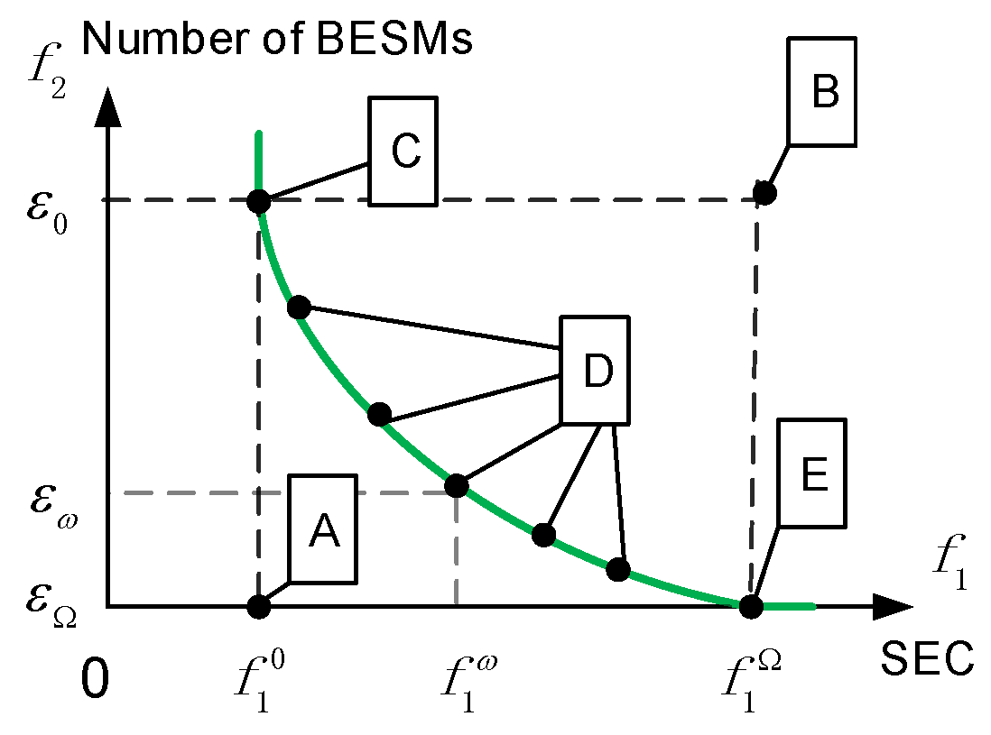
The results obtained by applying an $ϵ$-constraint method are illustrated in Figure 6. Point A is the ideal point and B is the nadir one of the dual-objective optimization problem. Points C and E are the end points on the Pareto front. Note that point D represents a typical point on the Pareto front. With ${ϵ}_{\omega }$ changes from ${ϵ}_0$ to ${ϵ}_{\mathsf{\Omega }}$, $f_1^{\omega }$ is changed from $f_1^0$ to $f_1^{\mathsf{\Omega }}$ correspondingly, thus point D can be any point on the green curve in Figure 6.

The procedure of applying an $ϵ$-constraint method to transform a dual-objective optimization problem P into several single-objective ones (i.e., problems $P_1$ to $P_5$) is detailed as follows. Note that the first objective in problem P (i.e., substation energy consumption) is treated as the primary objective.

• Obtain problems $P_1$ and $P_2$ respectively, where problem $P_1$ dismisses the second objective in problem P and problem $P_1$ dismisses the other one. The constraints in problem P are kept unchanged in both problems $P_1$ and $P_2$.
• By solving problem $P_1$, we obtain the minimal value of the first objective (i.e., substation energy consumption) without consideration of the other objective (WESS cost). The result is illustrated as $f_1^0$ in Figure 6. Similarly, by solving problem $P_2$, we obtain the minimal value of the second objective without consideration of the other one. the result is illustrated as ${ϵ}_{\mathsf{\Omega }}$.
• Obtain problem $P_3$ by adding constraint (35) into obtaining problem $P_2$. Note that the constraint is the first objective function in problem P and $f_1^0$ is the optimized result of problem $P_1$.
• By solving problem $P_3$, we obtain the minimal value of WESS size needed (denoted as ${ϵ}_0$) whilst maintaining minimum substation energy consumption. Note that ($f_1^0$, ${ϵ}_0$) is a non-dominated point of problem P, shown as point C in Figure 6.
• Obtain problem $P_4$ by adding constraint constraint (36) into obtain problem $P_1$. Note that the constraint is the second objective function in problem P and ${ϵ}_{\mathsf{\Omega }}$ is the optimized result of problem $P_2$.
• By solving problem $P_4$, we obtain the minimal value of substation energy consumption (denoted as $f_1^{\mathsf{\Omega }}$) whilst the least size of WESS is installed. Note that ($f_1^{\mathsf{\Omega }}$, ${ϵ}_{\mathsf{\Omega }}$) is also a non-dominated point of problem P, shown as point E in Figure 6.
• Obtain problem $P_5$ by adding constraint constraint (37) into obtain problem $P_1$. Note that the constraint is the second objective function in problem P and ${ϵ}_{\omega }$ is a variable which changes from ${ϵ}_0$ to ${ϵ}_{\mathsf{\Omega }}$ with a predefined step length. For different values of ${ϵ}_{\omega }$, it becomes a different problem. Thus, problem $P_5$ represents a series of optimization problems actually.
• By solving problem $P_5$ with each value of ${ϵ}_{\omega }$, we obtain a set of minimal values of substation energy consumption (denoted as $f_1^{\omega }$) whilst certain size of WESS (i.e., totally ${ϵ}_{\omega }$ number of BESMs) is installed. Note that each ($f_1^{\omega }$, ${ϵ}_{\omega }$) is a non-dominated point of problem P, shown as point D in Figure 6. Also note that point D actually represents a set of points in the green curve, as ${ϵ}_{\omega }$ is a changing from ${ϵ}_0$ to ${ϵ}_{\mathsf{\Omega }}$.

4.2. Improved Artificial Bee Colony Algorithm

For the single-objective optimization problems transformed from problem P, except $P_2$, all the other problems (i.e., $P_1$, $P_3$, $P_4$ and $P_5$) are nonlinear. It is hard to find an optimal solution by using commercial software (e.g., CPLEX) within an acceptable time. Thus, heuristic algorithms are often used to find near-optimal solutions for these kinds of problems [8,10,17,18,19,20,21,22,23,24,25].

An Artificial Bee Colony (ABC) algorithm is a swarm intelligence algorithm. Since 2005 [51], it has been successfully used to handle many complicated optimization problems [52,53,54,55,56,57,58]. It has been compared with differential evolution (DE) [59,60], GA [25,53,61], particle swarm optimization (PSO) [62,63] and evolutionary algorithm (EA) [64] for multi-dimensional numeric problems. Its performance is better than or similar to these algorithms. Therefore, An improved artificial bee colony algorithm is designed to solve the single-objective optimization problems in this work.

The proposed IABC starts with an initial set of feasible solutions, where one of them is the currently used timetable with no WESS, and the others are randomly generated. There are three kinds of bees, i.e., employed, onlooker and scout bees, used in an optimization process. In each iteration, each employed bee is employed at a particular solution, and finds a neighbor one via a local search operator, which is randomly chosen from swap, insertion, mutation and crossover operators; each onlooker bee chooses a solution by spinning a roulette wheel, and then finds a neighbor one with the same procedure as an employed bee; each scout bee randomly generates a feasible solution, to enhance IABC’s global search ability. the best solution found by all bees is kept as an initial one in the next iteration. When the iteration count reaches a predefined threshold, the algorithm restarts. Note that all the solutions, except the best one found, are replaced by randomly generated ones. IABC terminates when the restart count reaches a predefined limit. Then, the best solution found is output as an optimal result. The main procedure of IABC is shown in Algorithm 2. The detailed procedure of IABC can also be found in our previous work in [7]. $n_1$, $n_2$ and $n_3$ are the numbers of employed, onlooker and scout bees, respectively; $n_4$ is the total number of all bees, i.e., $n_4=n_1+n_2+n_3$; $p_1$, $p_2$, $p_3$ and $p_4$ are the probability of swap, insertion, mutation and crossover operators been chosen, respectively; $M_1$ and $M_2$ are predefined iteration count limits; ${\mathit{S}}^{*}$ is a specified initial solution; ${\mathit{S}}_{\mathbf{1}},{\mathit{S}}_{\mathbf{2}},\cdots ,$ and ${\mathit{S}}_{{\mathit{n}}_{\mathbf{4}}+\mathbf{1}}$ are one of $n_4+1$ solutions, respectively; ${\mathit{S}}^{{}^{\prime }}$ and $F^{{}^{\prime }}$ are the optimal solution found and its fitness value, respectively.

Algorithm 2 Procedure of IABC

Input:$n_1$, $n_2$, $n_3$, $n_4$, $p_s$, $p_i$, $p_m$, $p_c$, $M_1$, $M_2$, ${\mathit{S}}^{*}$ Output:${\mathit{S}}^{{}^{\prime }},F^{{}^{\prime }}$ 1: Set ${\mathit{S}}_{{\mathit{n}}_{\mathbf{4}}+\mathbf{1}}={\mathit{S}}^{*}$; %init the best solution found 2: for$j=1$ to $M_1\times M_2$ do 3:  if $(jmod{M}_2)=1$ then 4:   for $k=1$ to $n_4$ do 5:    Randomly generate a feasible solution ${\mathit{S}}_{\mathit{k}}$; 6:   end for 7:  end if 8:  for $k=1$ to $n_4+1$ do 9:   Calculate the fitness value $F_k$ for each solution ${\mathit{S}}_{\mathit{k}}$; 10:  end for 11:  Sort $F_1$, $F_2$, ⋯, $F_{n_4+1}$ in ’descend’ order and pick out the first $n_1$ number of elements to generate a list $\mathit{F}$; 12:  Generate a list $\overline{\mathit{S}}$ containing the $n_1$ number of solutions corresponding to $\mathit{F}$; 13:  Set ${\mathit{S}}_{{\mathit{n}}_{\mathbf{4}}+\mathbf{1}}$ = ${\overline{\mathit{S}}}_{\left(\mathbf{1}\right)}$; %record the best solution 14:  Set $F_{n_4+1}={\mathit{F}}_{\left(1\right)}$; %Fitness value of the best solution  %employed bee phase 15:  for $k=1$ to $n_1$ do 16:   Set solution $\mathit{B}={\overline{\mathit{S}}}_{\left(\mathit{k}\right)}$; 17:   Generate ${\mathit{S}}_{\mathit{k}}$ from $\mathit{B}$ via a local search operator randomly chosen from swap, insertion, mutation and crossover; 18:  end for  %onlooker bee phase 19:  for $k=1$ to $n_2$ do 20:   Set $\mathit{B}$ as a solution in $\overline{\mathit{S}}$ by roulette wheel selection; 21:   Generate ${\mathit{S}}_{{\mathit{n}}_{\mathbf{1}}+\mathit{k}}$ from $\mathit{B}$ via a local search operator randomly chosen from swap, insertion, mutation and crossover; 22:  end for  %scout bee phase 23:  for $k=1$ to $n_3$ do 24:   Randomly generate a feasible solution ${\mathit{S}}_{{\mathit{n}}_{\mathbf{1}}+{\mathit{n}}_{\mathbf{2}}+\mathit{k}}$; 25:  end for 26: end for 27: Output ${\mathit{S}}^{{}^{\prime }}={\mathit{S}}_{{\mathit{n}}_{\mathbf{4}}+\mathbf{1}}$ and $F^{{}^{\prime }}=F_{n_4+1}$;

The currently used timetable without WESS is used as an initial solution and the idea of elitism is adopted in IABC, to ensure the optimized solution is not getting worse than it. In each iteration, all solutions are evaluated and sorted based on their fitness values. A list containing $n_1$ best solutions is generated accordingly. Then, each employed bee is assigned to a specific solution in the list sequentially, and a new solution is generated by applying a local search operator. The local search operator is randomly chosen from swap, insertion, mutation and crossover operators with the probability of $p_1$, $p_2$, $p_3$ and $p_4$, respectively. To ensure each newly generated solution is feasible, i.e., satisfying constraints (28)–(34), its feasibility is checked immediately and repair is applied if it is infeasible. Similarly, each onlooker bee generates a new solution based on an assigned solution in the same way. The difference between employed and onlooker bees is as follows: the former is associated with a particular solution in the best solution list, and the latter randomly chooses one in the list by spinning a roulette wheel. A scout bee randomly generates a feasible solution in each iteration to ensure the global search ability of IABC. IABC converges to a local optimum in $M_2$ iterations. Then, the best solution found so far is kept and the other solutions are replaced by randomly generated feasible ones, to reduce the chance of IABC being trapped in a local optimum. Thereafter, a similar process repeats until the total iteration count reaches $M_1\times M_2$. Finally, a near-optimal solution and its fitness value are obtained.

5. Experimental Results and Analysis

To show the effectiveness of the proposed method, numerical examples are conducted based on the actual data obtained from Yanfang Line in Beijing, China. The actual dwell time at each platform and running time at each section are shown in

Table 1. Actual dwell time and running time of Yanfang Line.

Departure Platform Index n	${\mathit{x}}_{\mathit{n}}$ (s)	$\underline{{\mathit{x}}_{\mathit{n}}}$ (s)	$\overline{{\mathit{x}}_{\mathit{n}}}$ (s)	Arrival Platform Index $\mathit{n}+1$	${\mathit{r}}_{\mathit{l}}$ (s)
1	30	25	35	2	129
2	30	25	35	3	98
3	30	25	35	4	117
4	30	25	35	5	135
5	25	20	30	6	139
6	30	25	35	7	84
7	30	25	35	8	128
8	30	25	35	9	141
9	30	25	35	10	136
10	30	25	35	11	124
11	30	25	35	12	83
12	30	25	35	13	140
13	25	20	30	14	132
14	30	25	35	15	117
15	30	25	35	16	96
16	30	25	35	17	119

. Note that $x_n$ is dwell time at a departure platform with index n, $\underline{x_n}$ and $\overline{x_n}$ being its lower and upper bounds in the optimization process, and $r_l$ is the running time from platform $x_n$ to $x_{n+1}$. They are the same for all trains. The headway time and other parameters of Yanfang Line are listed in

Table 2. Other Parameters of Yanfang Line.

Parameter	Value	Parameter	Value	Parameter	Value
I	131	N	9	m (kg)	287,080
h (s)	482	$\underline{h}$ (s)	422	$\overline{h}$ (s)	542
${\eta }_1$	$0.7$	${\eta }_2$	$0.8$	${\zeta }_1$	$0.05$
$\tau$ (s)	2576	$\underline{\tau }$ (s)	2516	$\overline{\tau }$ (s)	2636
$\mathsf{\Phi }$ (s)	188	$a_l^1$	$0.8$	$a_l^3$ (m/s2)	1
$C_1$ (s)	65236	$r_l^1$ (s)	27	$r_l^3$ (s)	21

. Note that headway time between any two successive trains is identical in the current timetable. The sections in each electricity supply interval are given in

Table 3. Electricity supply intervals distribution of Yanfang Line.

Electricity Supply Interval Index	Section Indices
1	8	9	-	-	-	-
2	5	6	7	10	11	12
3	3	4	13	14	-	-
4	1	2	15	16	-	-

. A super-capacitor is selected as a BESM in this work. Parameters about WESS are shown in

Table 4. Parameters about WESS.

Parameter	Value	Parameter	Value	Parameter	Value
$P^m$ (kW)	2000	$C^m$ (kWh)	1	${\zeta }_2$	1
$\underleftarrow{P_z^c}$ (kW)	300	$\underleftarrow{P_z^d}$ (kW)	300	${\zeta }_3$	$0.1$
${\beta }_2$ (%)	90	${\beta }_1$ (%)	30	${\beta }_0$ (%)	20

.

Parameters of IABC are set as shown in

Table 5. Parameters of IABC.

${\mathit{n}}_{\mathit{e}}$	${\mathit{n}}_{\mathit{o}}$	${\mathit{n}}_{\mathit{s}}$	${\mathit{M}}_1$	${\mathit{M}}_2$	${\mathit{p}}_{\mathit{s}}$	${\mathit{p}}_{\mathit{i}}$	${\mathit{p}}_{\mathit{m}}$	${\mathit{p}}_{\mathit{c}}$
10	10	20	6	50	$0.1$	$0.1$	$0.2$	$0.6$

. GA is also applied to solve the single-objective optimization problems as a baseline method. The detailed processes of GA can be found in [21]. To compare IABC and GA fairly, the population size of GA is set to be 40 and its maximum iteration count is 300. The local search operators used in GA include selection, crossover and mutation. The probability of crossover and mutation are $0.8$ and $0.2$, respectively.

Compared with identical dwell time, more energy can be saved when dwell time at a platform varied for different trains. But regenerative energy utilization improvement is relatively limited, and it increases the solution space of an optimization problem dramatically [25]. Thus, in order to simplify the problem and keep consistent with the actual timetable, we keep the dwell time for different trains i and j at platform n identical in the experiments. i.e., $x_{i,n}=x_{j,n}$, $\forall i,j\in \{1,2,\dots ,I\}$ and $n\in \{1,2,\dots ,N-1\}$.

The experiments are implemented in MATLAB 2014 and runs on a notebook with Intel(R) Core(TM) i5-3210M CPU @$2.50$ GHz, 12 GB RAM and a Windows 7 Operating System.

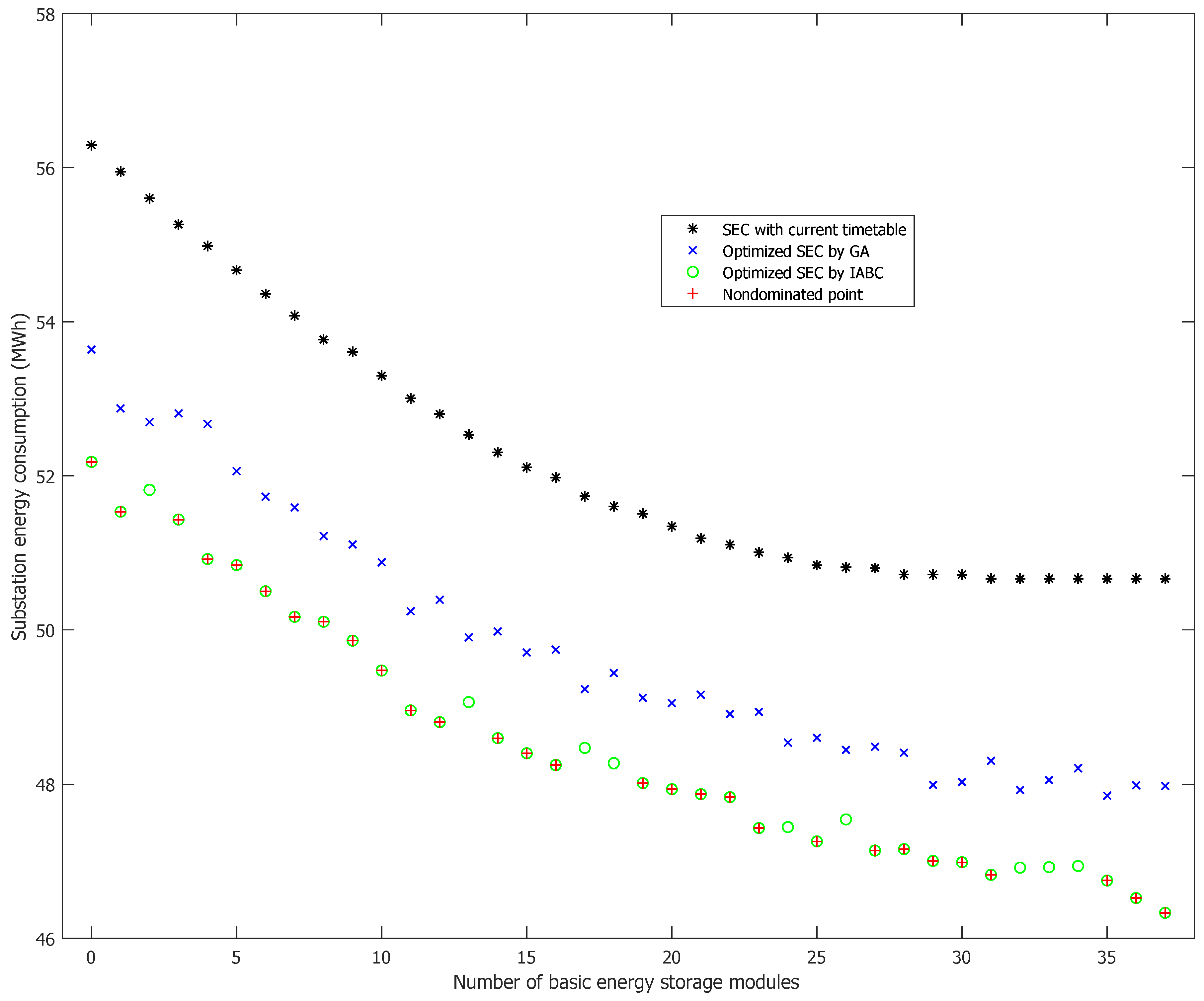
The simulation results are are shown in Figure 7. Note that there are several WESS in a subway line, different WESS may have different number of BESMs. The horizontal axis in Figure 7 is the sum of the BESM numbers in each WESS. The number of BESMs equals 0 means there are no WESS installed at all. When it is greater than 0, the detailed configuration in each WESS should be obtained in the optimized solution. The vertical axis is the substation energy consumption. A black asterisk in Figure 7 denotes substation energy consumption with the current timetable (i.e., the timetable is not optimized). Note that the configuration of each WESS is set as the optimized result, as there does not exist an actual configuration of WESS for each case. A blue cross denotes an optimized result obtained by GA where timetable and WESS are simultaneously optimized, a green circle denotes an optimized result of our dual-objective optimization problem obtained by IABC, and a red “+ “ in a green circle denotes a non-dominated point on the Pareto front of problem P.

From the experimental results, it is easy to see that: (1) Substation energy consumption decreases with the total size of WESS increases, and the decreasing speed gradually slows down. (2) With the same size of WESS installed, timetable optimization further reduces substation energy consumption, which shows the effectiveness of the integration optimization of timetable and WESS. (3) IABC and GA can both to solve the single-objective optimization problems, and IABC performs better than GA, as the results obtained by IABC dominate those obtained by GA. (4) A set of Pareto optimal solutions of the dual-objective optimization problem is obtained by applying the proposed $ϵ$-constraint method and IABC. The non-dominated points are diverse and well distributed over the Pareto front.

Set the current timetable with no WESS installed, which is the actual conditions in the experimental subway line, as a basis for comparison, substation energy consumption reduces by $(56.293-52.180)/56.293\times 100\%=7.31\%$ when timetable is optimized without WESS invested, optimization of WESS with total size as 37 BESMs reduces substation energy consumption by $(56.293-50.663)/56.293\times 100\%=10.00\%$ when timetable is optimized, and the decrement comes to $(56.293-46.331)/56.293\times 100\%=17.70\%$ when timetable is optimized together with 37 BESMs installed as WESS. Thus, timetable optimization and WESS installation can both improve energy conservation, and the integration of them reaches the greatest extent. Note that the results we obtained is a set of Pareto optimal solutions, each element of them reduces substation energy consumption to different degrees with different WESS investment cost. The experimental results are helpful for optimal decision making. Based on relationship between energy conservation profit and WESS cost, decision makers can easily choose a preferred solution according to their particular needs, e.g., the solution with the lowest cost, the one with the greatest profit, or that with the best cost-effectiveness.

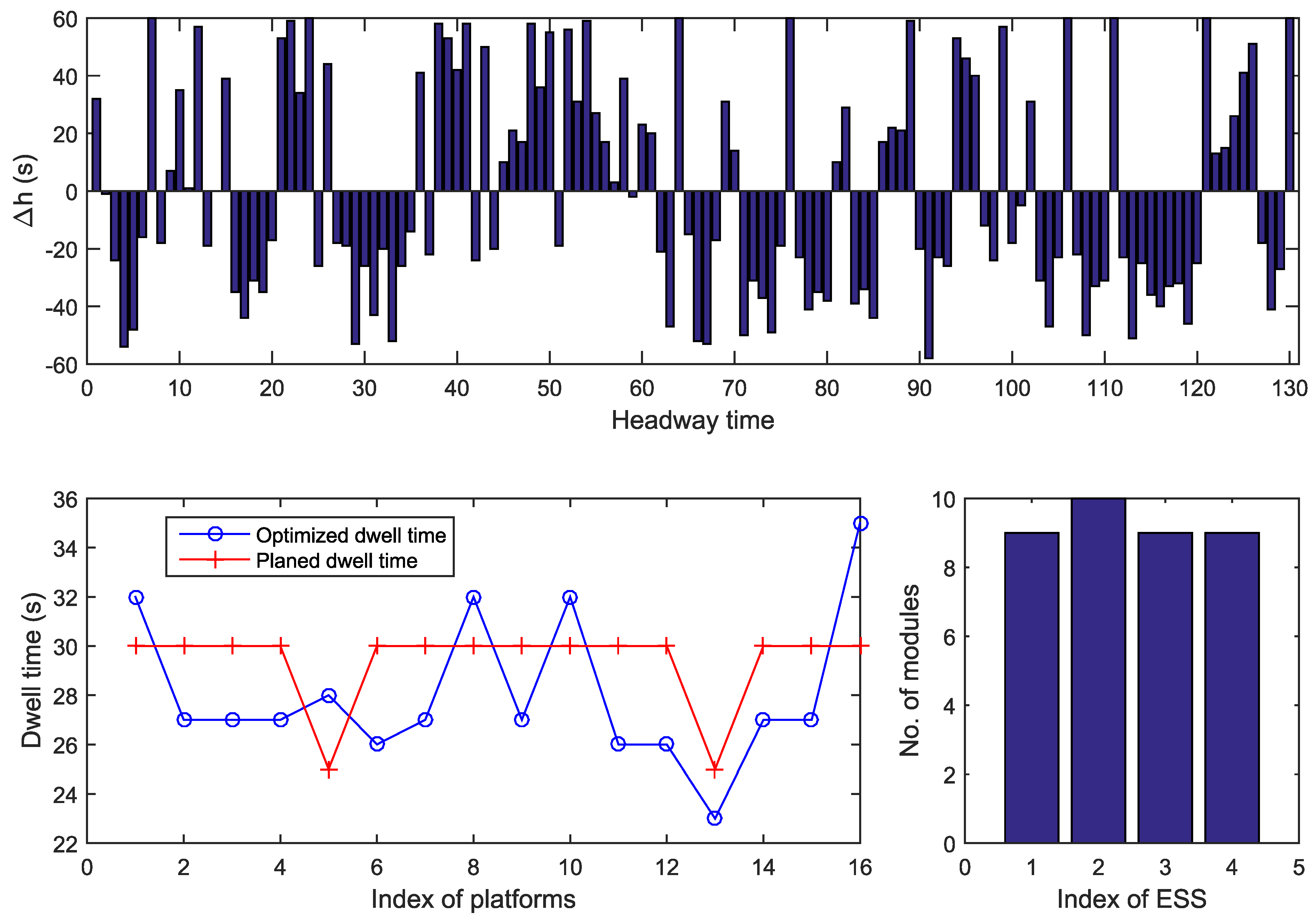
As an illustration of one optimized solution, the optimized timetable and configuration of each WESS when the total number of BESMs as $K=37$ are given in Figure 8. The upper part shows the difference between the optimized headway time and that in the current timetable; the lower left part shows the optimized dwell time and the current dwell time; in addition, the lower right part shows the numbers of BESMs in each WESS, note that there are four electricity supply intervals in this subway line, which means four WESSs are installed. It is seen that the headway time and dwell time are slightly changed from the current timetable, and the configuration for each WESS is proposed. Note that there are several electricity supply intervals in a subway system, and one WESS is installed in an electricity supply interval. Thus, there are several WESSs in a subway system (e.g., WESS 1 to z). As each WESS is independent from others, they can have different capacities (i.e., number of BESMs) in theory.

The profiles of the state-of-charge of each WESS are shown in Figure 9. The peak values of all WESS are between 90–100%. There is some residual capacity, but it is very small. Thus, this kind of WESS configuration is reasonable for regenerative energy utilization, i.e., if the total number of BESMs is reduced, some regenerative energy may not be able to be utilized; and if the number was increased, the increased energy capacity would be a waste of money.

A real-world subway line is often subject to minor real-time perturbations which affects the adherence to the timetable [7,17]. The presence of unexpected disturbances brings uncertainties to scheduling optimization problems [65,66], which may affect the effectiveness of the optimized results. To make it clear, the problem and method proposed in this work are intended to be used offline indeed, which means the optimization problem is solved only once before trains go into operation and the potential uncertainties are not particularly considered. However, the offline method is still of great significance, as the size of each WESS is hard to be changed over time; it should be decided at the first stage of design.

To solve the potential uncertainties in real-world application, there are two alternative ways. One is to adopt a real-time optimization method [65,66], e.g., using a receding horizon principle to optimize the timetable iteratively; the other is to evaluate the robustness of the optimized results on disturbances and subject to it if acceptable (i.e., the optimized results are not too sensitive to disturbances). It is relatively complicated to introduce an online optimization method in this work, so we leave it as our future work direction and adopt the second method here.

To evaluate the robustness of the optimized timetable, we conduct the following experiments by adding random noise to it. In the experiment, we traverse the headway time and dwell time vector and add a random number to each element in it. The random number is randomly chosen from set $\left\{-\delta ,0,\delta \right\}$ (s), which represents an actual noise. As a comparison, we add this king of noise both on the current timetable and the optimized one, and $\delta$ is assigned with different values to compare their effects on energy conservation. To be justified, we run the experiment 100 times with each value of $\delta$ and their average substation energy consumption is obtained, respectively. The experimental results with $\delta$ varies from 0 to 3 are given in

Table 6. Substation energy consumption (SEC) for timetable with noise.

Noise $\mathit{\delta }$ (s)	SEC with Current Timetable (kWh)	SEC with Optimized Timetable (kWh)	Energy Saving Ratio
0	56,293	46,331	17.70%
1	56,302	46,418	17.55%
2	56,313	46,592	17.26%
3	56,233	46,925	16.55%

.

Note that $\delta =0$ represents no noise added on the timetable. It is seen that the energy saving ratio slightly decreases when the disturbance on train operations becomes larger. However, even with 3-s of noise, the energy saving ratio is still around $17\%$ for the optimized timetable over the current one. Thus, the optimized result is robust enough for energy conservation under disturbances. The proposed offline optimization method is obviously acceptable to this particular problem.

6. Conclusions

We propose an integration of timetable optimization and WESS to improve regenerative energy utilization, thus to reduce substation energy consumption in a subway system. A dual-objective optimization model is formulated to simultaneously minimize substation energy consumption and WESS investment cost accordingly. To solve the dual-objective optimization problem, an $ϵ$-constraint method is first designed to transform it into several single-objective optimization problems; then, an improved artificial bee colony algorithm is designed to solve them sequentially. By combining the proposed $ϵ$-constraint method and improved artificial bee colony algorithm, a set of Pareto optimized solutions for the original dual-objective optimization can be obtained. Experiments based on the actual data from a subway system in China are conducted to illustrate the procedure to use them and their effectiveness. The results are useful for decision makers in a subway system, based on which they can easily make a sensible trade-off between energy saving profit and WESS investment cost according to their practical needs. In addition, the proposed improved artificial bee colony algorithm is also compared with a commonly used genetic algorithm during the experiments to prove its effectiveness.

The proposed model and resolution method can be used in any subway system which is equipped with regenerative braking systems, to maximize energy saving with the minimum investment cost paid for that. Although the optimized results are robust enough to random disturbances, one limit of the proposed method is that it is mainly applicable for offline optimization now. Thus, part of our future work will be the study of an online optimization method, to better handle the parameter uncertainty problems caused by unexpected disturbances to train operations. In addition, train speed profiles at sections also affect regenerative energy utilization and substation energy consumption. Thus, in our future research, we also plan to integrate energy-efficient train operations into our model to further reduce substation energy consumption.

References

1. González-Gil, A.; Palacin, R.; Batty, P.; Powell, J. A systems approach to reduce urban rail energy consumption. Energy Convers. Manag. 2014, 80, 509–524. [Google Scholar] [CrossRef]
2. González-Gil, A.; Palacin, R.; Batty, P. Optimal energy management of urban rail systems: Key performance indicators. Energy Convers. Manag. 2015, 90, 282–291. [Google Scholar] [CrossRef]
3. Yang, X.; Li, X.; Ning, B.; Tang, T. A survey on energy-efficient train operation for urban rail transit. IEEE Trans. Intell. Transp. Syst. 2016, 17, 2–13. [Google Scholar] [CrossRef]
4. Su, S.; Tang, T.; Wang, Y. Evaluation of strategies to reducing traction energy consumption of metro systems using an optimal train control simulation model. Energies 2016, 9, 105. [Google Scholar] [CrossRef]
5. Liu, R.R.; Golovitcher, I.M. Energy-efficient operation of rail vehicles. Transp. Res. Part A Policy Pract. 2003, 37, 917–932. [Google Scholar] [CrossRef]
6. Su, S.; Tang, T.; Roberts, C. A cooperative train control model for energy saving. IEEE Trans. Intell. Transp. Syst. 2015, 16, 622–631. [Google Scholar] [CrossRef]
7. Liu, H.; Zhou, M.; Guo, X.; Zhang, Z.; Ning, B.; Tang, T. Timetable optimization for regenerative energy utilization in subway systems. IEEE Trans. Intell. Transp. Syst. 2018, 1–11. [Google Scholar] [CrossRef]
8. Yang, X.; Ning, B.; Li, X.; Tang, T. A two-objective timetable optimization model in subway systems. IEEE Trans. Intell. Transp. 2014, 15, 1913–1921. [Google Scholar] [CrossRef]
9. González-Gil, A.; Palacin, R.; Batty, P. Sustainable urban rail systems: Strategies and technologies for optimal management of regenerative braking energy. Energy Convers. Manag. 2013, 75, 374–388. [Google Scholar] [CrossRef]
10. Kampeerawat, W.; Koseki, T. A strategy for utilization of regenerative energy in urban railway system by application of smart train scheduling and wayside energy storage system. Energy Procedia 2017, 138, 795–800. [Google Scholar] [CrossRef]
11. Ceraolo, M.; Lutzemberger, G.; Meli, E.; Pugi, L.; Rindi, A.; Pancari, G. Energy storage systems to exploit regenerative braking in dc railway systems: Different approaches to improve efficiency of modern high-speed trains. J. Energy Storage 2018, 16, 269–279. [Google Scholar] [CrossRef]
12. Ciccarelli, F.; Iannuzzi, D.; Tricoli, P. Control of metro-trains equipped with onboard supercapacitors for energy saving and reduction of power peak demand. Transp. Res. Part C Emerg. Technol. 2012, 24, 36–49. [Google Scholar] [CrossRef]
13. Ramos, A.; Pena, M.T.; Fernandez, A.; Cucala, P. Mathematical programming approach to underground timetabling problem for maximizing time synchronization. In Proceedings of the International Conference on Industrial Engineering and Industrial Management, Madrid, Spain, 5–7 September 2007; IEEE: Piscataway, NJ, USA, 2007; pp. 88–95. [Google Scholar]
14. Nasri, A.; Moghadam, M.F.; Mokhtari, H. Timetable optimization for maximum usage of regenerative energy of braking in electrical railway systems. In Proceedings of the International Symposium on Power Electronics Electrical Drives Automation and Motion, Pisa, Italy, 14–16 June 2010; IEEE: Piscataway, NJ, USA, 2010; pp. 1218–1221. [Google Scholar]
15. Kim, K.M.; Kim, K.T.; Han, M.S. A model and approaches for synchronized energy saving in timetabling. In Proceedings of the 9th World Congress on Railway Research, Lille, France, 22–26 May 2011. [Google Scholar]
16. Pe na-Alcaraz, M.; Fernández, A.; Cucala, A.P.; Ramos, A.; Pecharromán, R.R. Optimal underground timetable design based on power flow for maximizing the use of regenerative-braking energy. Proc. Inst. Mech. Eng. Part F J. Rail Rapid Transit 2012, 226, 397–408. [Google Scholar] [CrossRef]
17. Fournier, D.; Mulard, D.; Fages, F. Energy optimization of metro timetables: A hybrid approach. In Proceedings of the 18th International Conference on Principles and Practice of Constraint Programming, Quebec City, QC, Canada, 8–12 October 2012; Springer: Berlin/Heidelberg, Germany, 2012; pp. 7–12. [Google Scholar]
18. Yang, X.; Li, X.; Gao, Z.; Wang, H.; Tang, T. A cooperative scheduling model for timetable optimization in subway systems. IEEE Trans. Intell. Transp. Syst. 2013, 14, 438–447. [Google Scholar] [CrossRef]
19. Zhao, L.; Li, K.; Su, S. A multi-objective timetable optimization model for subway systems. In Proceedings of the 2013 International Conference on Electrical and Information Technologies for Rail Transportation (EITRT2013)—Volume I; Springer: Berlin/Heidelberg, Germany, 2014; pp. 557–565. [Google Scholar]
20. Le, Z.; Li, K.; Ye, J.; Xu, X. Optimizing the train timetable for a subway system. Proc. Inst. Mech. Eng. Part F J. Rail Rapid Transit 2015, 229, 852–862. [Google Scholar] [CrossRef]
21. Yang, X.; Chen, A.; Li, X.; Ning, B.; Tang, T. An energy-efficient scheduling approach to improve the utilization of regenerative energy for metro systems. Transp. Res. Part C Emerg. Technol. 2015, 57, 13–29. [Google Scholar] [CrossRef]
22. Li, X.; Lo, H.K. Energy minimization in dynamic train scheduling and control for metro rail operations. Transp. Res. Part B Methodol. 2014, 70, 269–284. [Google Scholar] [CrossRef]
23. Gong, C.; Zhang, S.; Zhang, F.; Jiang, J.; Wang, X. An integrated energy-efficient operation methodology for metro systems based on a real case of shanghai metro line one. Energies 2014, 7, 7305–7329. [Google Scholar] [CrossRef]
24. Xu, X.; Li, K.; Li, X. A multi-objective subway timetable optimization approach with minimum passenger time and energy consumption. J. Adv. Transp. 2016, 50, 69–95. [Google Scholar] [CrossRef]
25. Liu, H.; Zhou, M.; Guo, X.; Liu, H.; Tang, T. An abc-based subway timetable optimization model for regenerative energy utilization. In Proceedings of the International Conference on Systems, Man, and Cybernetics, Miyazaki, Japan, 7–10 October 2018; IEEE: Piscataway, NJ, USA, 2018; pp. 1412–1417. [Google Scholar]
26. Tian, Z.; Weston, P.; Zhao, N.; Hillmansen, S.; Roberts, C.; Chen, L. System energy optimisation strategies for metros with regeneration. Transp. Res. Part C Emerg. Technol. 2017, 75, 120–135. [Google Scholar] [CrossRef]
27. Liu, H.; Tang, T.; Guo, X.; Xia, X. A timetable optimization model and an improved artificial bee colony algorithm for maximizing regenerative energy utilization in a subway system. Adv. Mech. Eng. 2018, 10, 1–13. [Google Scholar] [CrossRef]
28. Liu, P.; Yang, L.; Gao, Z.; Huang, Y.; Li, S.; Gao, Y. Energy-efficient train timetable optimization in the subway system with energy storage devices. IEEE Trans. Intell. Transp. Syst. 2018, 19, 1–17. [Google Scholar] [CrossRef]
29. Gao, Z.; Fang, J.; Zhang, Y.; Sun, D. Control strategy for wayside supercapacitor energy storage system in railway transit network. J. Mod. Power Syst. Clean Energy 2014, 2, 181–190. [Google Scholar] [CrossRef]
30. Huang, Y.; Yang, L.; Tang, T.; Gao, Z.; Cao, F.; Li, K. Train speed profile optimization with on-board energy storage devices: A dynamic programming based approach. Comput. Ind. Eng. 2018, 126, 149–164. [Google Scholar] [CrossRef]
31. Ahmadi, S.; Dastfan, A.; Assili, M. Energy saving in metro systems: Simultaneous optimization of stationary energy storage systems and speed profiles. J. Rail Transp. Plan. Manag. 2018, 8, 78–90. [Google Scholar] [CrossRef]
32. Wu, P.; Che, A.; Chu, F.; Zhou, M. An improved exact varepsilon-constraint and cut-and-solve combined method for biobjective robust lane reservation. IEEE Trans. Intell. Transp. Syst. 2015, 16, 1479–1492. [Google Scholar] [CrossRef]
33. Chankong, V.; Haimes, Y.Y. Multiobjective Decision Making: Theory and Methodology; North-Holland: New York, NY, USA, 1983. [Google Scholar]
34. Carli, R.; Dotoli, M. Energy scheduling of a smart home under nonlinear pricing. In Proceedings of the 53rd IEEE Conference on Decision and Control, Los Angeles, CA, USA, 15–17 December 2014; IEEE: Piscataway, NJ, USA, 2014; pp. 5648–5653. [Google Scholar]
35. Carli, R.; Dotoli, M. Cooperative distributed control for the energy scheduling of smart homes with shared energy storage and renewable energy source. IFAC-PapersOnLine 2017, 50, 8867–8872. [Google Scholar] [CrossRef]
36. Sperstad, I.B.; Korpås, M. Energy storage scheduling in distribution systems considering wind and photovoltaic generation uncertainties. Energies 2019, 12, 1231. [Google Scholar] [CrossRef]
37. T’kindt, V.; Billaut, J.-C. Multicriteria scheduling problems: A survey. RAIRO-Oper. Res. 2001, 35, 143–163. [Google Scholar] [CrossRef]
38. Zhou, Z.; Chu, F.; Che, A.; Zhou, M. ε-constraint and fuzzy logic-based optimization of hazardous material transportation via lane reservation. IEEE Trans. Intell. Transp. Syst. 2013, 14, 847–857. [Google Scholar] [CrossRef]
39. Guo, X.; Liu, S.; Zhou, M.; Tian, G. Disassembly sequence optimization for large-scale products with multiresource constraints using scatter search and petri nets. IEEE Trans. Cybern. 2016, 46, 2435–2446. [Google Scholar] [CrossRef]
40. Guo, X.; Liu, S.; Zhou, M.; Tian, G. Dual-objective program and scatter search for the optimization of disassembly sequences subject to multiresource constraints. IEEE Trans. Autom. Sci. Eng. 2018, 15, 1091–1103. [Google Scholar] [CrossRef]
41. Sun, H.; Wu, J.; Ma, H.; Yang, X.; Gao, Z. A bi-objective timetable optimization model for urban rail transit based on the time-dependent passenger volume. IEEE Trans. Intell. Transp. Syst. 2018, 20, 1–12. [Google Scholar] [CrossRef]
42. Ehrgott, M. Multicriteria Optimization; Springer Science & Business Media: Berlin/Heidelberg, Germany, 2005; p. 491. [Google Scholar]
43. Haimes, Y.Y.; Lasdon, L.; Wismer, D. On a bicriterion formulation of the problems of integrated system identification and system optimization. IEEE Trans. Syst. Man Cybern. 1971, 1, 296–297. [Google Scholar]
44. Berube, J.-F.; Gendreau, M.; Potvin, J.-Y. An exact ε-constraint method for bi-objective combinatorial optimization problems: Application to the traveling salesman problem with profits. Eur. J. Oper. Res. 2009, 194, 39–50. [Google Scholar] [CrossRef]
45. Feng, J.; Che, A.; Wang, N. Bi-objective cyclic scheduling in a robotic cell with processing time windows and non-euclidean travel times. Int. J. Prod. Res. 2014, 52, 2505–2518. [Google Scholar] [CrossRef]
46. Jozefowiez, N.; Semet, F.; Talbi, E.-G. The bi-objective covering tour problem. Comput. Oper. Res. 2007, 34, 1929–1942. [Google Scholar] [CrossRef]
47. Leitner, M.; Ljubic, I.; Sinnl, M. Solving the bi-objective prizecollecting steiner tree problem with the varepsilon-constraint method. Electron. Notes Discret. Math. 2013, 41, 181–188. [Google Scholar] [CrossRef]
48. Reiter, P.; Gutjahr, W.J. Exact hybrid algorithms for solving a bi-objective vehicle routing problem. Cent. Eur. J. Oper. Res. 2012, 20, 19–43. [Google Scholar] [CrossRef]
49. Bouziaren, S.A.; Aghezzaf, B. An improved augmented varepsilon-constraint and branch-and-cut method to solve the tsp with profits. IEEE Trans. Intell. Transp. Syst. 2018, 20, 1–10. [Google Scholar]
50. Marler, R.T.; Arora, J.S. Survey of multi-objective optimization methods for engineering. Struct. Multidiscip. Optim. 2004, 26, 369–395. [Google Scholar] [CrossRef]
51. Karaboga, D. An Idea Based on Honey Bee Swarm for Numerical Optimization; Technical Report-tr06; Erciyes University, Engineering Faculty, Computer Engineering Department: Kayseri, Turkey, 2005. [Google Scholar]
52. Deng, G.; Xu, Z.; Gu, X. A discrete artificial bee colony algorithm for minimizing the total flow time in the blocking flow shop scheduling. Chin. J. Chem. Eng. 2012, 20, 1067–1073. [Google Scholar] [CrossRef]
53. Li, J.; Pan, Q.; Gao, K. Pareto-based discrete artificial bee colony algorithm for multi-objective flexible job shop scheduling problems. Int. J. Adv. Manuf. Technol. 2011, 55, 1159–1169. [Google Scholar] [CrossRef]
54. Gu, W.; Yu, Y.; Hu, W. Artificial bee colony algorithm-based parameter estimation of fractional-order chaotic system with time delay. IEEE/CAA J. Autom. Sin. 2017, 4, 107–113. [Google Scholar] [CrossRef]
55. Singh, A. An artificial bee colony algorithm for the leaf-constrained minimum spanning tree problem. Appl. Soft Comput. 2009, 9, 625–631. [Google Scholar] [CrossRef]
56. Pan, Q.-K.; Tasgetiren, M.F.; Suganthan, P.; Chua, T. A discrete artificial bee colony algorithm for the lot-streaming flow shop scheduling problem. Inf. Sci. 2011, 181, 2455–2468. [Google Scholar] [CrossRef]
57. Karaboga, D.; Basturk, B. On the performance of artificial bee colony (abc) algorithm. Appl. Soft Comput. 2008, 8, 687–697. [Google Scholar] [CrossRef]
58. Karaboga, D.; Akay, B. A comparative study of artificial bee colony algorithm. Appl. Math. Comput. 2009, 214, 108–132. [Google Scholar] [CrossRef]
59. Tian, G.; Ren, Y.; Zhou, M. Dual-objective scheduling of rescue vehicles to distinguish forest fires via differential evolution and particle swarm optimization combined algorithm. IEEE Trans. Intell. Transp. Syst. 2016, 17, 3009–3021. [Google Scholar] [CrossRef]
60. Wang, L.; Wang, S.; Zheng, X. A hybrid estimation of distribution algorithm for unrelated parallel machine scheduling with sequence-dependent setup times. IEEE/CAA J. Autom. Sin. 2016, 3, 235–246. [Google Scholar]
61. Mareda, T.; Gaudard, L.; Romerio, F. A parametric genetic algorithm approach to assess complementary options of large scale windsolar coupling. IEEE/CAA J. Autom. Sin. 2017, 4, 260–272. [Google Scholar] [CrossRef]
62. Dong, W.; Zhou, M. A supervised learning and control method to improve particle swarm optimization algorithms. IEEE Trans. Syst. Man Cybern. Syst. 2017, 47, 1135–1148. [Google Scholar] [CrossRef]
63. Tang, Y.; Luo, C.; Yang, J.; He, H. A chance constrained optimal reserve scheduling approach for economic dispatch considering wind penetration. IEEE/CAA J. Autom. Sin. 2017, 4, 186–194. [Google Scholar] [CrossRef]
64. Kang, Q.; Feng, S.; Zhou, M.; Ammari, A.C.; Sedraoui, K. Optimal load scheduling of plug-in hybrid electric vehicles via weight-aggregation multi-objective evolutionary algorithms. IEEE Trans. Intell. Transp. Syst. 2017, 18, 2557–2568. [Google Scholar] [CrossRef]
65. Hosseini, S.M.; Carli, R.; Dotoli, M. Model predictive control for real-time residential energy scheduling under uncertainties. In Proceedings of the 2018 IEEE International Conference on Systems, Man, and Cybernetics (SMC), Miyazaki, Japan, 7–10 October 2018; IEEE: Piscataway, NJ, USA, 2018; pp. 1386–1391. [Google Scholar]
66. Touretzky, C.R.; Baldea, M. Integrating scheduling and control for economic mpc of buildings with energy storage. J. Process. 2014, 24, 1292–1300. [Google Scholar] [CrossRef]
Figure 1. Main ideas of this work.
Energies 12 01876 g001
Figure 2. Train travel process.
Energies 12 01876 g002
Figure 3. General process of a subway train running at a section.
Energies 12 01876 g003
Figure 4. Energy suppliers and consumers in an electricity supply interval.
Energies 12 01876 g004
Figure 5. Maximum charging and discharging power of WESS.
Energies 12 01876 g005
Figure 6. Points obtained by an ϵ -constraint method.
Energies 12 01876 g006
Figure 7. Traction energy saved in different numbers of basic energy storage modules.
Energies 12 01876 g007
Figure 8. One optimized timetable and WESS configuration.
Energies 12 01876 g008
Figure 9. State-of-charge of each WESS.
Energies 12 01876 g009