Article

Adaptive Air-Fuel Ratio Regulation for Port-Injected Spark-Ignited Engines Based on a Generalized Predictive Control Method

1
School of Automation, Wuhan University of Technology, Wuhan 430070, China
2
Department of Electrical Engineering, University of South Carolina, Columbia, SC 29208, USA
*
Authors to whom correspondence should be addressed.
Energies 2019, 12(1), 173; https://doi.org/10.3390/en12010173
Submission received: 8 December 2018 / Revised: 1 January 2019 / Accepted: 3 January 2019 / Published: 6 January 2019

Abstract

:
The accurate air-fuel ratio (AFR) control is crucial for the exhaust emission reduction based on the three-way catalytic converter in the spark ignition (SI) engine. The difficulties in transient cylinder air mass flow measurement, the existing fuel mass wall-wetting phenomenon, and the unfixed AFR path dynamic variations make the design of the AFR controller a challenging task. In this paper, an adaptive AFR regulation controller is designed using the feedforward and feedback control scheme based on the dynamical modelling of the AFR path. The generalized predictive control method is proposed to solve the problems of inherent nonlinearities, time delays, parameter variations, and uncertainties in the AFR closed loop. The simulation analysis is investigated for the effectiveness of noise suppression, online prediction, and self-correction on the SI engine system. Moreover, the experimental verification shows an acceptable performance of the designed controller and the potential usage of the generalized predictive control in AFR regulation application.

1. Introduction

The port-injected spark ignition (SI) engine is widely used in automotive production vehicles, which is equipped with a three-way catalytic converter (TWC) to reduce the exhaust emissions. The combination of the TWC and electronic fuel injection control have been developed for SI engines to meet the strict emission requirements. Using the TWC can reduce nitrogen oxides to nitrogen and oxygen, oxidize carbon monoxide to carbon dioxide, and oxidize hydrocarbons to carbon dioxide and water. However, the TWC conversion efficiency depends on the exhaust air–fuel ratio (AFR) significantly. To guarantee the maximum converter efficiency and fuel economy, the AFR is required to regulate at a very narrow band around the stoichiometric value. For the most widely used port-injected SI engine in the in-use vehicles, the emission performance could be improved using the advanced AFR control method.
For accurate AFR control, correct estimation of the intake air mass in the cylinder, the right amount of fuel injection, and the closed-loop AFR regulation based on the exhaust gas oxygen (EGO) sensor are three main practical aspects [1]. However, it is hard to measure the transient cylinder air mass by sensors due to the intake manifold dynamic variations. The injected fuel mass before the intake valve is not equal to the fuel mass in the cylinder as the wall-wetting phenomenon [2]. Otherwise, the inherent nonlinearities, time delays, parameter variations, existed uncertainties, the complex engine operating conditions, and tremendous measurement noise make the design of the AFR controller a challenging task and has captured enormous attention recently.
Practically, the AFR controller consists of feed-forward look-up tables and the feedback proportional–integral–derivative (PID) controller. The look-up tables are calibrated at different engine operating conditions for open loop control, and the PID controller compensates the output error based on the EGO sensor measurement. Although this traditional control scheme is stable, the calibration of look-up tables and gain parameters of the PID controller are time-consuming and may not guarantee the control performance due to the engine aging and parameters varying. The dramatic variations of the exhaust equivalence ratio can be a challenging problem for traditional PID controllers as they are not robust to nonlinearity and uncertainties [3]. Many approaches have been proposed in the literature regarding the AFR control using advanced methods [4]. Model-based AFR controllers were implemented in Reference [5,6] using the mean-value engine model by event-based discrete sampling method. A backstepping controller [7] was designed for the AFR regulation to solve the problem of unknown input time delay and unknown parameters in the plant. Linear parameter-varying control [8,9], sliding mode control [10,11], and a Smith predictor [12] were introduced to improve the AFR regulation performance. As it is hard to describe the exact AFR path dynamic with certain models and parameters, using adaptive control [1,12,13] for the AFR regulation aroused interest regarding the control issue. A new method of AFR calculation was carried out in Reference [14] using fast response CO and CO2 sensors. However, the existing works have less consideration on the actual AFR dynamic variations.
In this paper, the AFR dynamical modelling and the specific problem of stoichiometric AFR regulation are investigated for the port-injected SI engine. The control strategy is designed based on the feedforward and feedback fueling controller via the mean-value engine model. An adaptive feedback controller is implemented using the generalized predictive control method to handle the AFR regulation difficulties. Using the simulation analysis and experimental validation, we investigate the effectiveness of the proposed method.

2. Modelling of Dynamic AFR of the SI Engine

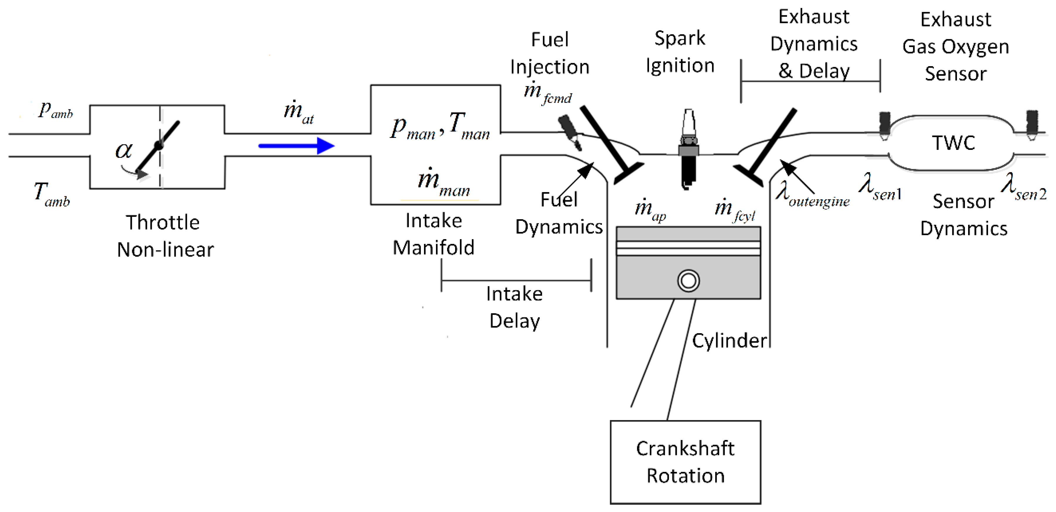
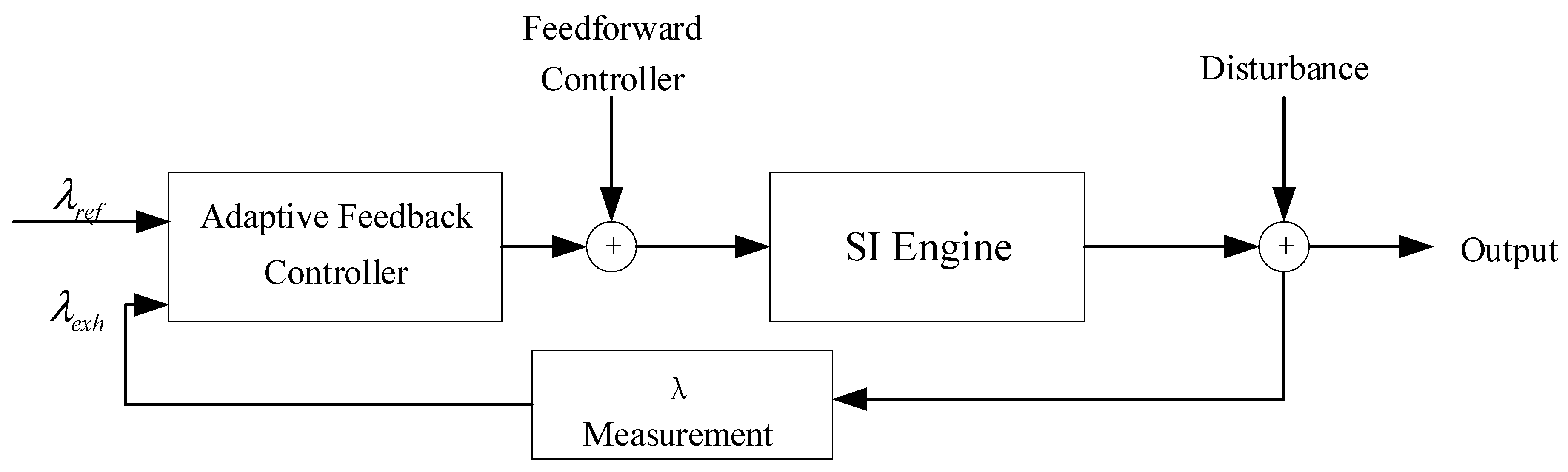
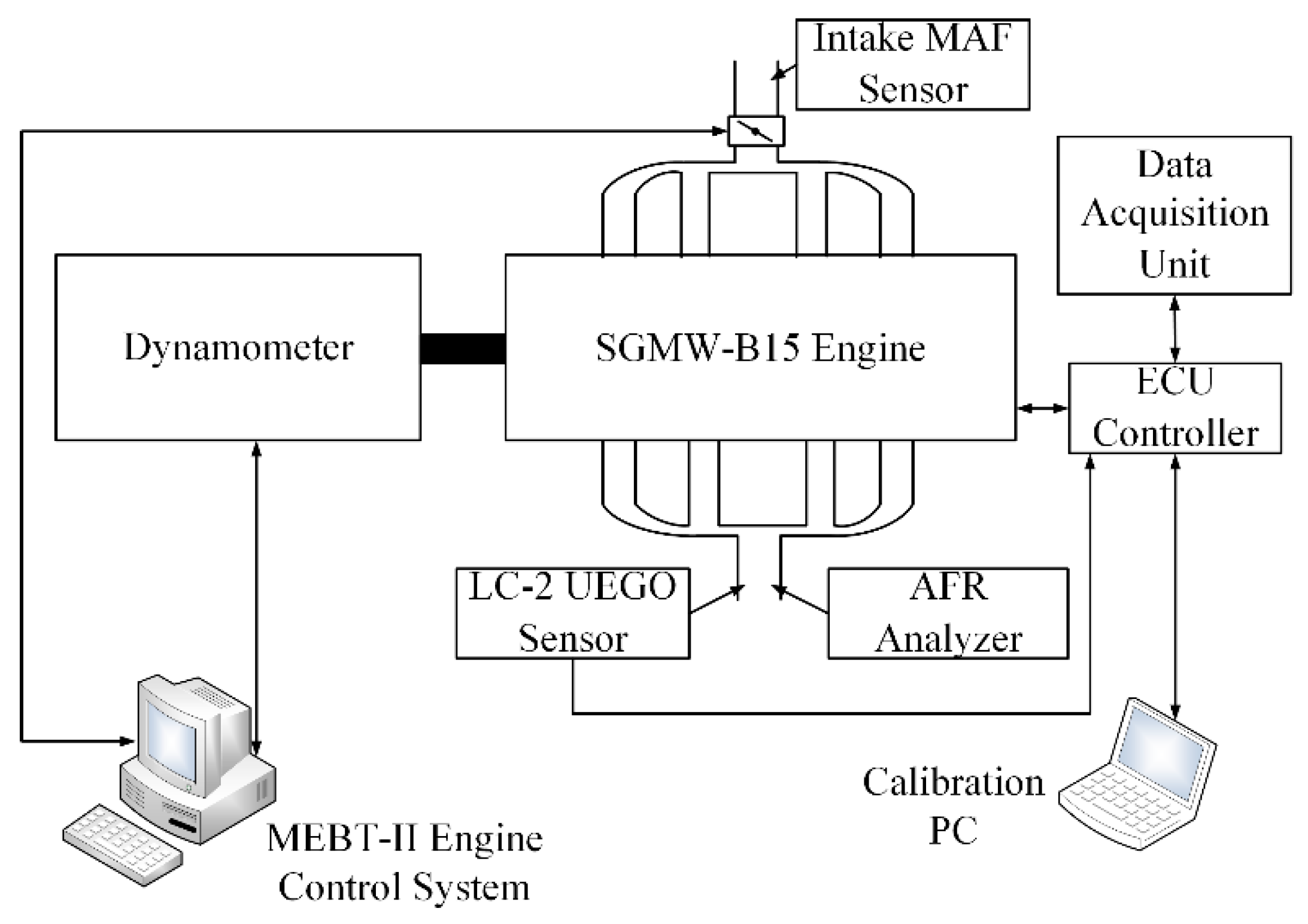
2.1. System Description

AFR means the ratio of the air ( m ˙ a p ) and fuel ( m ˙ f c y l ) mass flow rate in the engine cylinder, and it is commonly given by the variable of λ which is the ratio of AFR and the stoichiometric ratio ( A F R s , approximately 14.7 for gasoline). The fuel/air equivalence ratio ( ϕ ) is a more informative parameter for defining the mixture composition and can be measured using the exhaust gas oxygen sensor (EGO). AFR parameters are determined using:
{ A F R = m ˙ a p m ˙ f c y l λ = A F R A F R s = 1 ϕ
AFR control is a fundamental issue in the internal combustion engine and has a strong impact on the combustion, efficiency, and emission performances. A brief structure of the AFR control system in the port injected SI engine is shown in Figure 1. The intake air and the injected fuel mix in the intake manifold is before the intake valves; then, the gas mixture enters the engine cylinder and is ignited by the spark plug to release the chemical energy. The combustion process in the expansion stroke produces the engine output torque. The SI engine is controlled by the throttle position angle ( α ), which affects the relative air mass supply. The electronic control unit (ECU) controls the amount of fuel injection ( m ˙ f c m d ) based on the intake air mass and AFR regulation strategy. However, the in-cylinder AFR could not be measured directly by sensors in commercial engine systems. The typical method uses the EGO sensor before the TWC to measure the oxygen content in the exhaust gas mixture ( ϕ e x h ) to represent the AFR during the combustion process.
Based on the definition, the intake air mass in each cylinder, the appropriate fuel injection amount, and the close-loop control are the main contents of the AFR regulation. It should be noted that the fuel mass in the cylinder should adapt the intake air mass based on the AFR definition. However, due to the immeasurability of the intake air mass in the cylinder and the fuel wall-wetting phenomenon, the challenge in the AFR control exists regarding how to handle the air charge mass, fuel dynamic characteristic, and AFR transmission process, especially during the transient operation mode. Moreover, the parameters of the air intake path and the fuel path are usually difficult to determine with certainty.

2.2. The Dynamic AFR in the SI Engine

The SI engine is a highly nonlinear and multi-variable system that is difficult to derive the precise model for the control purpose. Typically, the computational fluid dynamics (CFD) model can provide the information of engine combustion performance and is too complex for the control application. The mean value engine model (MVEM) is suitable for real-time simulation and has acceptable accuracy for representing engine dynamics for the control application [15,16]. The MVEM describes the physical engine dynamics on the time scale of several engine events without the cycle-to-cycle characteristics. It consists of three dynamic mathematical subsystem models including the air path, fuel path, and crankshaft. As the AFR control parameters depend on engine operating conditions, the dynamic AFR is specifically analyzed in this section based on MVEM.

2.2.1. The Air Path Dynamic Model

The intake air dynamic model expresses the manifold filling with air mass through the throttle plate ( m ˙ a t ), while at the same time air mass is drawn into the engine ( m ˙ a p ). Based on the ideal gas law, the manifold pressure state equation in the form [17,18]:
p ˙ m a n = R T m a n V m a n ( m ˙ a t m ˙ a p )
where V m a n is the volume of the intake manifold (L); R is the gas constant of fresh air (287 J/(kg∙K)); T m a n is the manifold air temperature (K); and p m a n is the manifold air pressure (kPa), which can be measured using the manifold absolute pressure (MAP) sensor. The air mass flow across the throttle can be physically modelled as two separated parallel isentropic flows [19]:
m ˙ a t = m ˙ a t 1 p a m b T a m b β 1 α β 2 p r p r = p m a n p i n β 1 α = 1 a 1 cos α + a 2 cos 2 α β 2 p r = 1 p n ( p r p 1 p r p 2 ) , if p r p c 1 , if p r < p c p c = p 1 p 2 1 p 2 p 1 p n = p c p 1 p c p 2
where p r is the ratio of air pressure before and after the throttle plate; m ˙ a t 1 is a fitting constant; α is the throttle opening angle (degree); β 1 ( α ) , β 2 ( p r ) are the empirical equations; p a m b and T a m b are the ambient air pressure and temperature; and a 1 , a 2 , p 1 , p 2 , p n , p c are constant parameters that have been found in Reference [19]. As the pressure and temperature in the engine cylinders cannot be measured in practice, it is difficult to use the ideal gas law to calculate the real air mass in the cylinder. Therefore, volumetric efficiency ( e v ) is introduced to observe the amount of air in each cylinder using the pressure and temperature measured in the manifold. Using the speed density formula:
m ˙ a p = V d 120 R T m a n ( e v p m a n ) n = V d 120 R T m a n ( s i p m a n y i ) n
where V d is the engine displacement (L); n is the engine velocity (RPM); and s i , y i are speed-dependent fitting parameters and should not change much over the engine operating range.

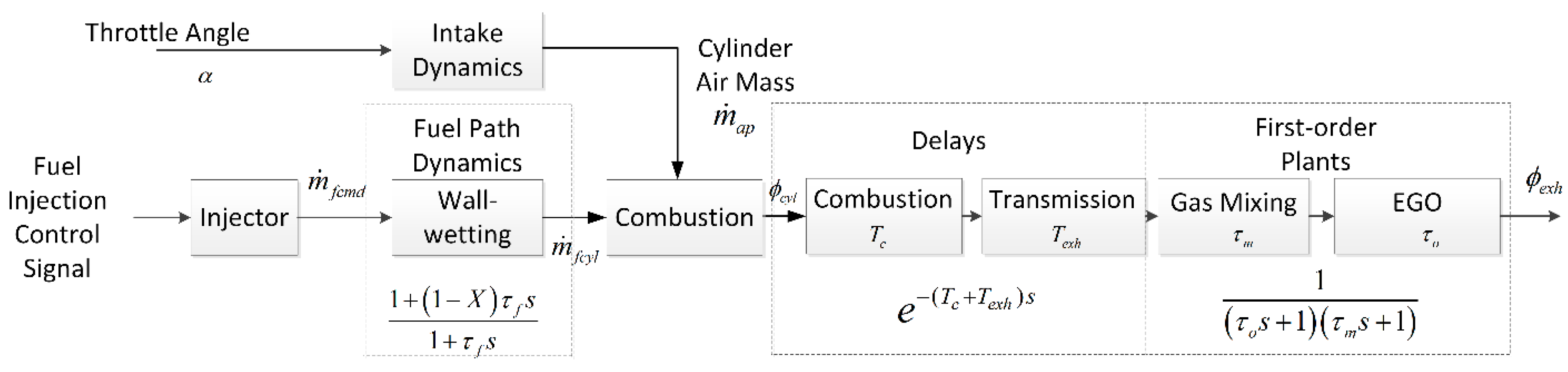
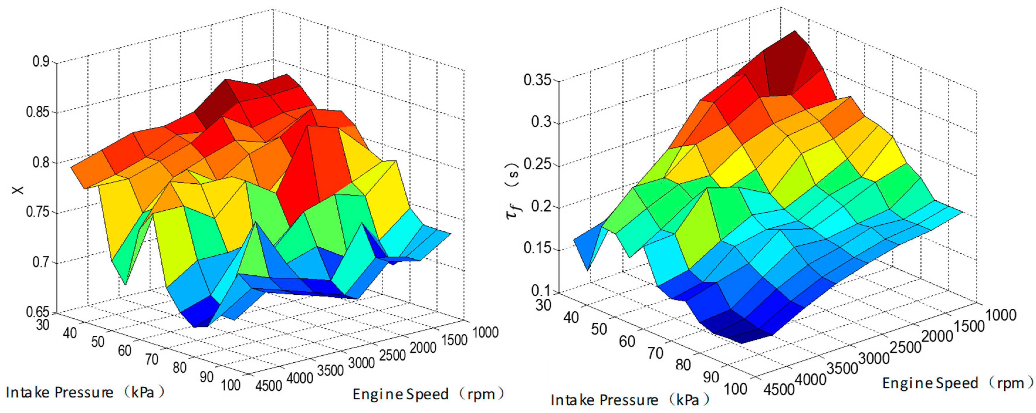
2.2.2. The Fuel Path Dynamic Model

As the wall-wetting phenomenon in port fuel injection engines discussed by Hendricks [20] occurs, a portion of the injected fuel out of the injector may form a fuel film on the intake manifold wall and the other may be as a vapor flow. Consequently, the total fuel, together with the air mass into the engine’s cylinder, is unequal to the injected fuel at each engine event. It consists of the fuel vapor flow from both the direct injection and the fuel film on the manifold wall. The fuel vapor and film dynamic variation can be described as:
{ m ¨ f f ( t ) = 1 τ f ( X m ˙ f c m d ( t ) m ˙ f f ( t ) ) m ˙ f v ( t ) = ( 1 X ) m ˙ f c m d ( t ) m ˙ f c y l ( t ) = m ˙ f v ( t ) + m ˙ f f ( t )
where the fraction of the fuel flow become film is defined as X ( 0 < X < 1 ), τ f is the fuel film evaporation time constant, m ˙ f c y l is the fuel mass flow entering the cylinder, m ˙ f c m d denotes the injected fuel mass flow following the control command, and m ˙ f v and m ˙ f f represent the fuel mass flow from the injection directly and the wall film evaporation, respectively. This model is a convenient approximation to the true physical dynamic of the fuel in the engine, and Equation (5) can be rewritten as a single transfer function for the controller design:
G w w ( s ) = m ˙ f c y l ( s ) m ˙ f c m d ( s ) = ϕ c y l ( s ) ϕ c m d ( s ) = 1 + ( 1 X ) τ f s 1 + τ f s

2.2.3. The Crankshaft Dynamic

As the energy conservation law, the change of the rotational kinetic energy causes by the available acceleration power on the crankshaft. The model can be described as:
{ ω ˙ = ( T i T f T l o a d ) / I = [ H u m ˙ f c y l ( t ) η i ( t τ d ) / ω T f T l o a d ] / I η i ( θ i , λ , n , p m a n ) = η i ( θ i ) η i ( λ ) η i ( n ) η i ( p m a n )
where ω is the engine velocity (rad/s); I is the associate moment of inertia both of the engine and load(kg∙m2); T i   , T f   , T l o a d are the torque of indicated, friction, and load, respectively; H u is the fuel heating value(J/kg); τ d is the delay between the change of speed and fuel flow step; η i is the indicated efficiency, which is affected by the spark advance angle ( θ i ), λ , crankshaft speed (n), and manifold air pressure.

2.2.4. AFR Path Dynamic Model

For the control purpose, the AFR path dynamic coves the process from the fuel injection to the measured exhaust equivalence ratio as shown in Figure 2. In this section, all the model parameters are analyzed based on a four-cylinder engine. Combustion delay ( T c ) indicates the time delay between the inlet and exhaust valve opening, T c = 3 4 × 120 n = 90 n for the four-stroke engine. The transmission delay represents the time of the exhaust gas reaching the sensor after combustion, and it varies depending on the air velocity. In this work, it is modeled as: T e x h = l v e x h T c = 90 n . The exhaust gas from each cylinder mixes in the tailpipe and can be modelled as a first-order plant [21], where the time constant is τ m and is approximately equal to three times the time slot between each different cylinder intake valve opening. Meanwhile, the EGO sensor can be modelled as a first-order plant [2], and the time constant τ o can be approximately 20 ms for a conventional sensor.
Based on the above description, the air mixture from the cylinder to the EGO sensor can be denoted as the series connection of several pure delay and first-order plants. As τ m τ o τ m + τ o , the transfer function can be rewritten as follow:
{ ϕ e x h ( s ) = e ( T c + T e x h ) s ϕ c y l ( s ) ( τ o s + 1 ) ( τ m s + 1 ) e ( T c + T e x h ) s ϕ c y l ( s ) ( τ o + τ m ) s + 1 = e τ d s ϕ c y l ( s ) τ e x h s + 1 τ d = T c + T e x h ,    τ e x h = τ o + τ m
Combining with Equations (4) and (6), the AFR dynamic can be approximately modeled as:
ϕ e x h ( s ) 1 m ˙ a p ( e τ d s τ e x h s + 1 1 + ( 1 X ) τ f s 1 + τ f s ) m ˙ f c m d ( s )

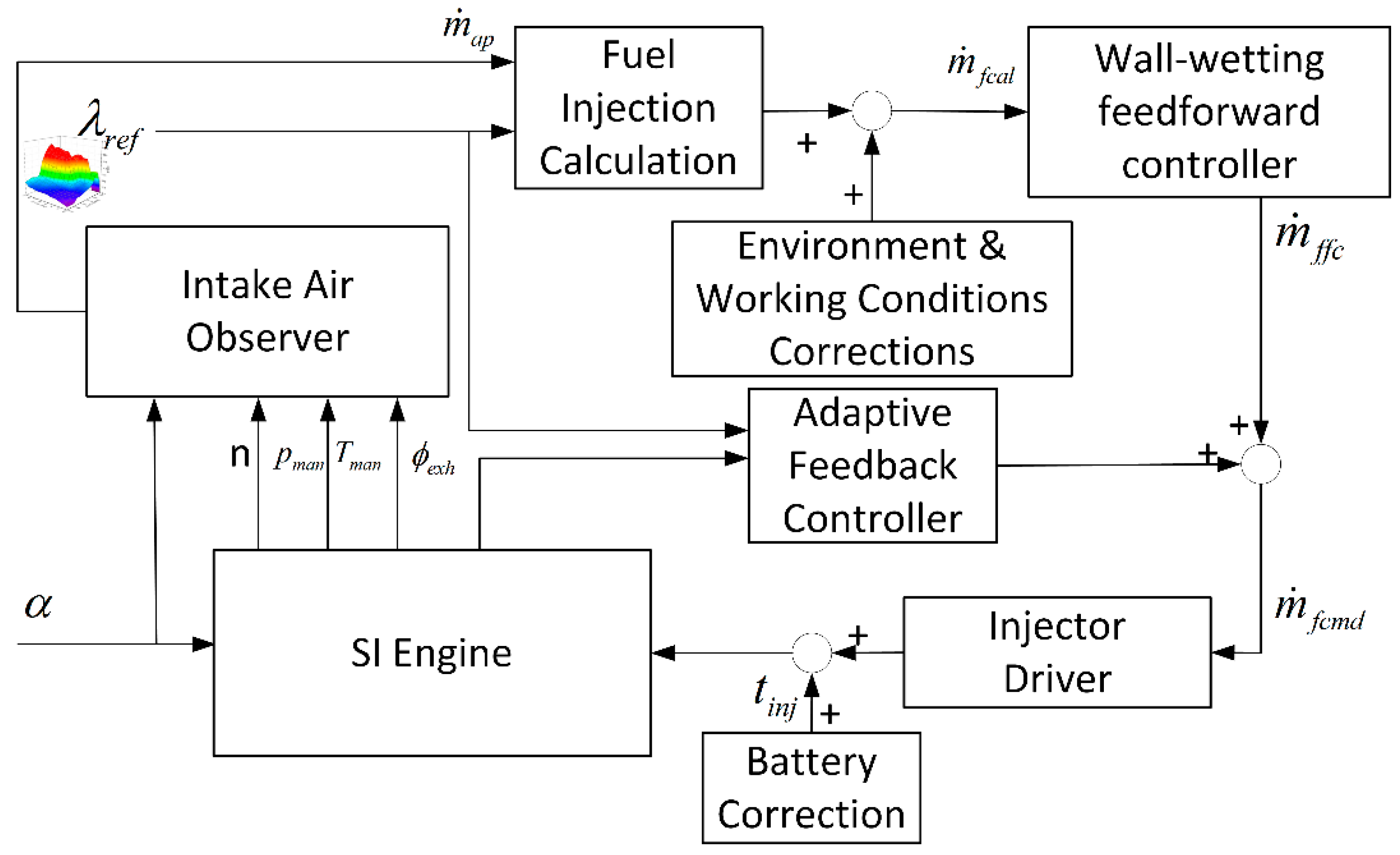
3. Adaptive AFR Regulation Controller Design

3.1. Problem Formulation of AFR Regulation

The engine speed and load can define the engine working conditions. The AFR control aims to regulate the air fuel mixture at a proper value under different operating conditions. At some power, preferred conditions, such as the transient accelerating or WOT (wide opening throttle), the air fuel mixture may be set to a rich condition for the immediate torque output and the AFR control may be set to the open-loop based on the control parameter value from the calibrated look-up table. Nevertheless, under most cases, such as the idle speed and steady operating conditions, the AFR control is closed-loop for the accuracy objective. As the controlling strategy is complicated and mostly based on the empirical experience, it will not be explained in detail in this paper. Only the closed-loop AFR controller design is focused in this work based on the exhaust equivalence ratio measured by a UEGO (universal exhaust gas oxygen) sensor. The design objective is to track a reference air-fuel ratio ( ϕ r e f ) and reject disturbances at different conditions. ϕ r e f is other than the stoichiometric value for calibration requirements in practice.
Although the SI engine can be modeled using an MVEM and the AFR dynamic is analyzed above, it is still challenging work to handle the control problems of parameter variations and uncertainties, the time-delay and nonlinearities, the large modeling uncertainties and unknown dynamics, and the wide operating range and complex working conditions. The typical analysis method for a SISO (single input single output) control system is not suitable for such a complex dynamic process. A proper AFR controller should control the engine to the reference air-fuel ratio as quickly as possible under flexible operating conditions and guarantee the static and transient performance. It also should have robustness against uncertain parameters and the disturbance rejection ability [1].
To overcome the problems mentioned above, an adaptive AFR controller design is introduced in this paper based on generalized predictive control method (GPC). GPC was first reported by Clarke [22] on the basis of self-tuning and adaptive control theories. It is capable of stable control of processes with variable parameters and effective with a nonminimum-phase and open-loop unstable plants. This control method suits the AFR regulation, which is a high-performance application of a complex system.
The designed scheme of the adaptive controller is shown in Figure 3, where the feedforward controller compensates the fuel wall-wetting dynamic characteristic and the feedback controller improves the quality of regulation of the feedforward control algorithm. An intake air observer is designed for the in-cylinder air mass estimation that is crucial for the fuel injection calculation. Some necessary corrections, such as the battery voltage of the injector, the environment parameters, and the operating conditions, are also presented, which are reserved for the accurate calibration in practical ECU design.

3.2. Observer-Based Intake Air Estimation

During the transient operation, the air mass flow passing through the throttle valve is not equivalent to the air mass into the cylinder because of the variation of the manifold pressure. However, the instantaneous air mass flow through the intake valve is difficult to measure directly. Practically, there are two kinds of methods to predict the intake air mass: one is the mass air flow (MAF) sensor method regarding direct measurement of the mass flow entering the intake system, the other is the manifold air pressure (MAP) sensor method based on the speed–density approach. Compared to the MAF sensor, the MAP sensor, which is widely used on existing engine control systems, costs less and has a faster response time. There are already many research works on the air charge estimation to improve the accuracy at both transient and steady state [23]. In this work, the intake air observer is developed based on the MAP sensor using the speed–density formula, and one MAF sensor is used to calibrate the parameter at steady state.

3.3. Wall-Wetting Feedforward Controller Design

By taking the wall-wetting effect discussed above into consideration, a fuel feedforward controller is developed to compensate for the in-cylinder fuel mass to the calculated amount based on the intake air and equivalence ratio as m ˙ f c y l ( t ) = m ˙ f c a l ( t ) . Therefore, the ideal transfer function of the controller is as below based on Equation (6):
G f f c ( s ) = m ˙ f f c ( s ) m ˙ f c a l ( s ) = 1 + τ f s 1 + ( 1 X ) τ f s
As X and τ are unable to be measured directly, the estimated controller dynamics takes the form:
G f f c ( s ) = 1 + τ ^ f s 1 + ( 1 X ^ ) τ ^ f s = 1 + X ^ τ ^ f s 1 + ( 1 X ^ ) τ ^ f s = 1 + G f f c 1 ( s )
G f f c 1 ( s ) can be reconstructed to the discrete-time domain using the zero-order sampled at T = 120 / n :
{ G f f c 1 ( z ) = Z [ ( 1 e T s s ) ( X ^ τ ^ f s 1 + ( 1 X ^ ) τ ^ f s ) ] = ( 1 z 1 ) Z [ X ^ τ ^ f 1 + ( 1 X ^ ) τ ^ f s ] = a a z 1 1 b z 1 a = X ^ 1 X ^ ;   b = e T ( 1 X ^ ) τ ^ f
The discrete controller can be rewritten as:
{ m ˙ f f c 1 ( k + 1 ) = a ( m ˙ f c a l ( k + 1 ) m ˙ f c a l ( k ) ) + b m ˙ f f c 1 ( k ) m ˙ f f c ( k + 1 ) = m ˙ f f c 1 ( k + 1 ) + m ˙ f c a l ( k + 1 )
It should be noted that the Z transform could not be used to handle the time-varying system. However, for the engine control application, the speed of the inner parameter varying is much less than the event-based sampling rate. Therefore, the system can be treated as a time-invariant system around each operating point. X ^ and τ ^ f were obtained via the parameter identification using the square wave perturbation experiment method [24] on the engine test bench as shown in Figure 4.

3.4. Adaptive Feedback Controller Design

The adaptive feedback controller uses the GPC method to regulate the AFR variation. The feedback control scheme is shown in Figure 5, where the feedforward control output can be treated as the disturbance. The effect of unknown dynamics, the noise, parameter varying, parameter unknown, and model error can be treated as the disturbance at the output. Consequently, the feedback control problem is simplified to the reference λ adaptive tracking problem under a different operation point.
In order to establish the controlled auto-regressive integrated moving average (CARIMA) model for the GPC controller design, the AFR dynamic should be described in the discrete-time domain as the natural engine operating process. Using zero-order hold to discretize Equation (8) at sampling time T , without regard to the pure delay section:
G ( z ) = Z [ ( 1 e T s s ) ( 1 τ e x h s + 1 ) ] = ( 1 z 1 ) Z [ 1 s ( τ e x h s + 1 ) ] = ( 1 z 1 ) ( 1 1 z 1 z z e T τ e x h ) = ( 1 e T τ e x h ) z 1 1 e T τ e x h z 1
Assuming the pure delay, τ d is the integer multiples of the sampling time, combined with the description of delay in Section 2.2.4, we have:
{ τ d c T ϕ c y l ( k c ) = ( 1 e T τ e x h ) 1 ( ϕ e x h ( k + 1 ) e T τ e x h ϕ e x h ( k ) )
By considering the one-event between the sampling of exhaust gas and the fuel injection, and also that Equation (6) can be discretized by the zero-order hold, the difference equation can be written:
m ˙ f c y l ( k ) e T τ f m ˙ f c y l ( k 1 ) = ( 1 X ) m ˙ f c m d ( k ) + ( X e T τ f ) m ˙ f c m d ( k 1 )
Assuming the air intake mass under steady state near the operating point follows:
( 1 e T τ f z 1 ) ϕ c y l ( k ) = 1 m ˙ a p ( ( 1 X ) + ( X e T τ f ) z 1 ) m ˙ f c m d ( k )
then, combining Equations (15) and (17) gives:
( 1 e T τ e x h ) 1 ( 1 e T τ e x h z 1 ) ϕ e x h ( k ) = 1 m ˙ a p ( 1 e T τ f z 1 ) 1 ( ( 1 X ) + ( X e T τ f ) z 1 ) m ˙ f c m d ( k c 1 )
Compared with the CARIMA model, A ( z 1 ) y ( k ) = B ( z 1 ) u ( k 1 ) + C ( z 1 ) ξ ( k ) / ( 1 z 1 ) , the model parameters can be as follows:
{ A ( z 1 ) = 1 + a 1 z 1 + + a n a z n a = 1 ( e T τ e x h + e T τ f ) z 1 + e ( T τ e x h + T τ f ) z 2 ; B ( z 1 )   = ( b 0 + b 1 z 1 + + b n b z n b ) = z c ( 1 X m ˙ a p + X e T τ f m ˙ a p z 1 ) ; C ( z 1 )   = 1 + c 1 z 1 + + c n c z n c = 1 ;
It can be found that the A ( z 1 ) and B ( z 1 ) are variable, and the parameters could be obtained using online identifications.
First, we consider a cost-function of the form:
J = E { j = N 0 N [ y ( k + j ) w ( k + j ) ] 2 + j = 1 N u γ j [ Δ u ( k + j 1 ) ] 2 }
where w ( k + j ) is the future set-point sequence, N 0 is the minimum costing horizon, N is the maximum costing horizon, N u is the control horizon, and γ j is a control-weighting sequence. In order to avoid the system output signal from strongly fluctuating, we define the set-point sequence as:
w ( k + j ) = α y ( k ) + ( 1 α ) y r
where y r is the referenced equivalence ratio, and 0 < α < 1 is the smoothing coefficient. This provides a smoothed approach from the current output to the desired reference output. The AFR regulation problem can be simplified to the control objective of obtaining the optimal Δ u ( k ) , Δ u ( k + 1 ) , , Δ u ( k + N u 1 ) to minimize the cost function, such that the system output can track the referenced exhaust equivalence ratio and limit the fuel mass injection fluctuating.
Second, the predictive control law is developed. A Diophantine equation is carried out here:
C ( z 1 ) = ( 1 z 1 ) A ( z 1 ) E j ( z 1 ) + z j G j ( z 1 ) = A ¯ ( z 1 ) E j ( z 1 ) + z j G j ( z 1 )
combined with the CARIMA model description:
A ¯ ( z 1 ) y ( k ) = B ( z 1 ) Δ u ( k 1 ) + C ( z 1 ) ξ ( k )
y ( k + j ) = B ( z 1 ) A ¯ ( z 1 ) Δ u ( k + j 1 ) + E j ( z 1 ) ξ ( k + j ) + G j ( z 1 ) A ¯ ( z 1 ) ξ ( k )
to define:
F j ( z 1 ) = B ( z 1 ) E j ( z 1 ) = L j ( z 1 ) C ( z 1 ) + z j H j ( z 1 )
such that the following equations can be obtained:
y ( k + j ) = F j ( z 1 ) C ( z 1 ) Δ u ( k + j 1 ) + E j ( z 1 ) ξ ( k + j ) + G j ( z 1 ) C ( z 1 ) y ( k )
y ( k + j ) = L j ( z 1 ) Δ u ( k + j 1 ) + H j ( z 1 ) C ( z 1 ) Δ u ( k 1 ) + G j ( z 1 ) C ( z 1 ) y ( k ) + E j ( z 1 ) ξ ( k + j )
Assuming C ( z 1 )   = 1 , the equations above can be written in the vector form:
Y ( k + j ) = L Δ U ( k ) + G Y ( k ) + H Δ U ( k j ) + E ξ ( k + j )
where the vectors are all N × 1 :
Y   ( k + j ) = [ y ( k + 1 ) , y ( k + 2 ) y ( k + N ) ] T Δ U ( k )   = [ Δ u ( k ) , Δ u ( k + 1 ) Δ u ( k + N u 1 ) ] T Δ U ( k j )   = [ Δ u ( k 1 ) , Δ u ( k 2 ) Δ u ( k n b ) ] T Y   ( k ) = [ y ( k ) , y ( k 1 ) y ( k n a ) ] T
where ξ ( k + j ) = [ ξ ( k + 1 ) , ξ ( k + 2 ) ξ ( k + N ) ] T is the noise vector; and L, G, H, E are from Equations (22) and (25). The cost-function in Equation (20) can be rewritten as:
J = E { [ Y ( k + j ) W ] T [ Y ( k + j ) W ] + λ Δ U   ( k ) T Δ U   ( k ) }
Assuming J / Δ U = 0 , we have:
Δ U   ( k ) = ( L T L + λ I ) 1 L T [ W H Δ U ( k j ) G Y ( k ) ]
such that the current control u ( k ) is given by:
u ( k ) = u ( k 1 ) + p T [ W H Δ U ( k j ) G Y ( k ) ]
where p T = [ p 1 , p N ] is the first row of ( L T L + λ I ) 1 L T .
However, the AFR dynamic is a parameter varying plant based on the analysis in Equation (19), where the system parameter is not constant. The adaptive control law is provided in Equation (31) which should rely on the CARIMA model. In order to use the estimations of A ^ ( z 1 )   , B ^ ( z 1 ) to implement the control law, it can be obtained using the online identification by forgetting factor recursive least squares. From CARIMA model definition, we have:
Δ y ( k ) = a 1 Δ y ( k 1 ) a n a Δ y ( k n a ) + b 0 Δ u ( k 1 ) + + b n b Δ u ( k n b 1 ) + ξ ( k )
Assuming:
{ ϕ T ( k 1 ) = [ Δ y ( k 1 ) , , Δ y ( k n a ) , Δ u ( k 1 ) , , Δ u ( k n b 1 ) ] θ = [ a 1 , a 2 , , a n a , b 0 , b 1 , , b n b ] T Δ y ( k ) = y ( k ) y ( k 1 )
Equation (32) can be rewritten as:
Δ y ( t ) = ϕ T ( k 1 ) θ + w ( t )
Using the forgetting factor ρ between 0.95 and 0.99, we have:
{ θ ^ ( k ) = θ ^ ( k 1 ) + P ( k 1 ) ϕ ( k 1 ) ρ + ϕ ( k 1 ) T P ( k 1 ) ϕ ( k 1 ) [ Δ y ( k ) ϕ T ( k 1 ) θ ^ ( k 1 ) ] P ( k ) = 1 ρ [ P ( k 1 ) P ( k 1 ) ϕ ( k 1 ) ϕ T ( k 1 ) P ( k 1 ) ρ + ϕ T ( k 1 ) P ( k 1 ) ϕ ( k 1 ) ]
where A ^ ( z 1 )   , B ^ ( z 1 ) can be obtained using θ ^   adaptively.
For the GPC controller implementation, choosing the control horizons defined by N , N u is crucial. In this application, the control horizon parameter is determined based on the simulation results. In general, N is chosen to encompass all the responses, which is significantly affected by the current control; it is reasonable that it should at least be greater than the degree of B ( z 1 ) for the consideration of the control stability and response speed [22]. In this work, we choose N = 6 . N u is equivalent to placing effectively infinite weights on control changes after some future time, N u < N . However, increasing N u makes the control and the corresponding output more active and better tracking performance with a more complex calculation. In this work, we choose N u = 2 . For simplicity in the derivation, the control-weighting γ is set to the constant.
In the application of AFR regulation, the control input of fuel injection should be positive and have the boundary of injector characteristics. The total amount of fuel injection from the feedback ( u ( k ) ) and feedforward controller ( u f f c ( k ) ) should meet u min u ( k ) + u f f c ( k ) u max . Therefore, the adaptive feedback controller output is as below:
u ( k ) = { u min u f f c ( k ) ,   w h e n   u ( k ) u f f ( k ) u max u f f c ( k )   ,   w h e n   u ( k ) u max u f f ( k ) u ( k ) ,   o t h e r s

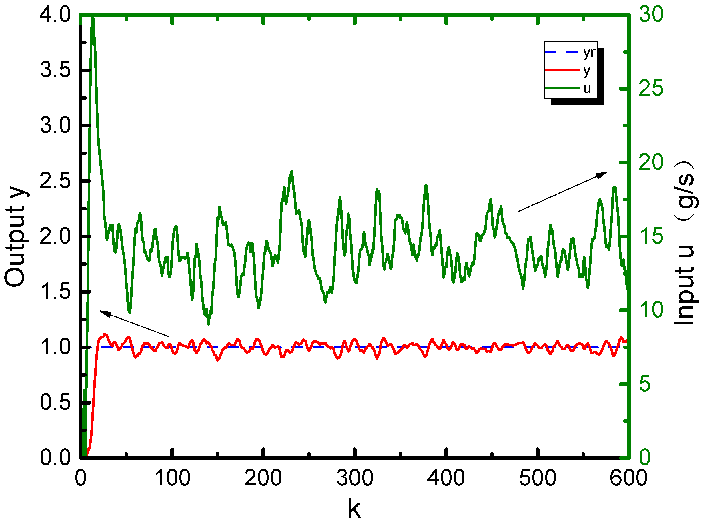
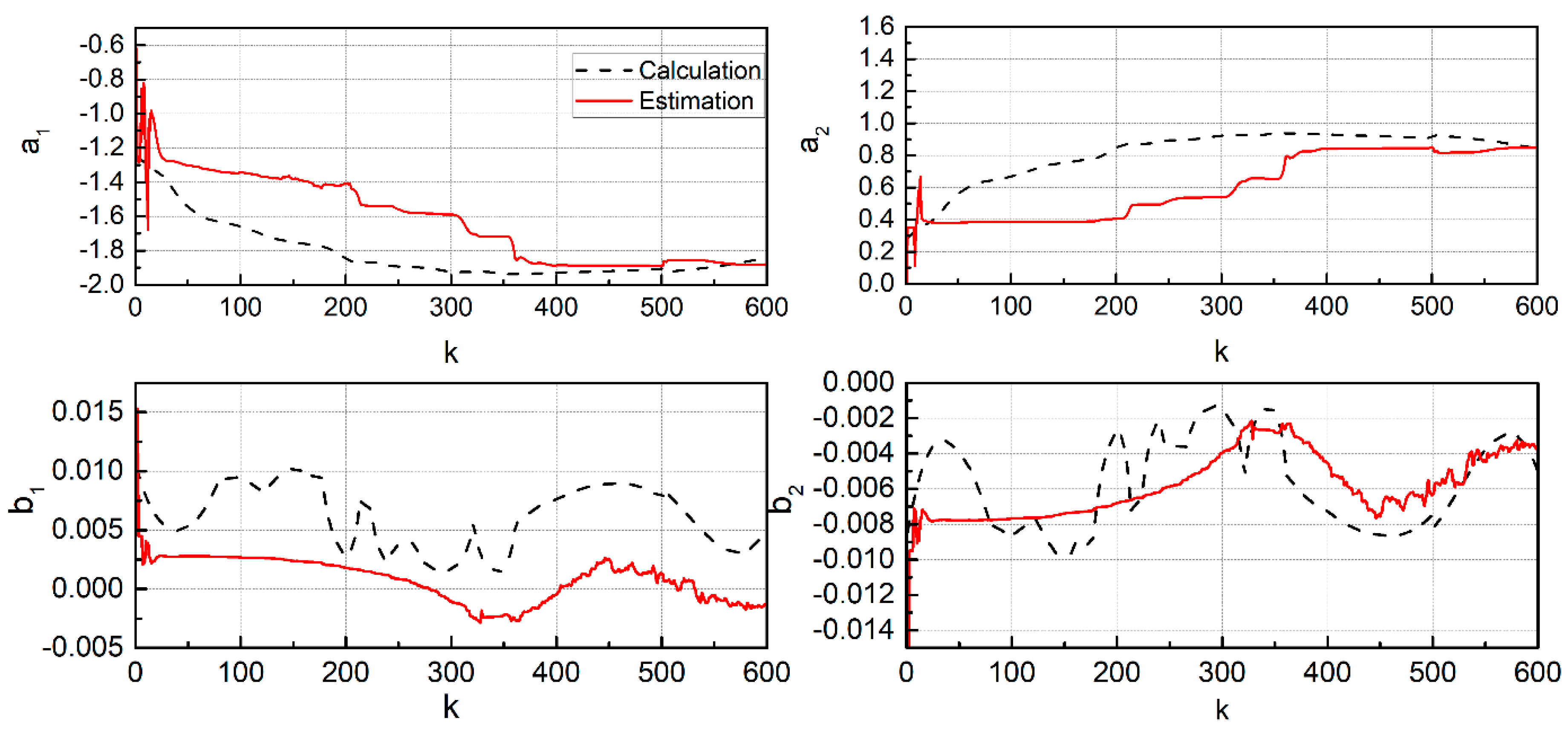
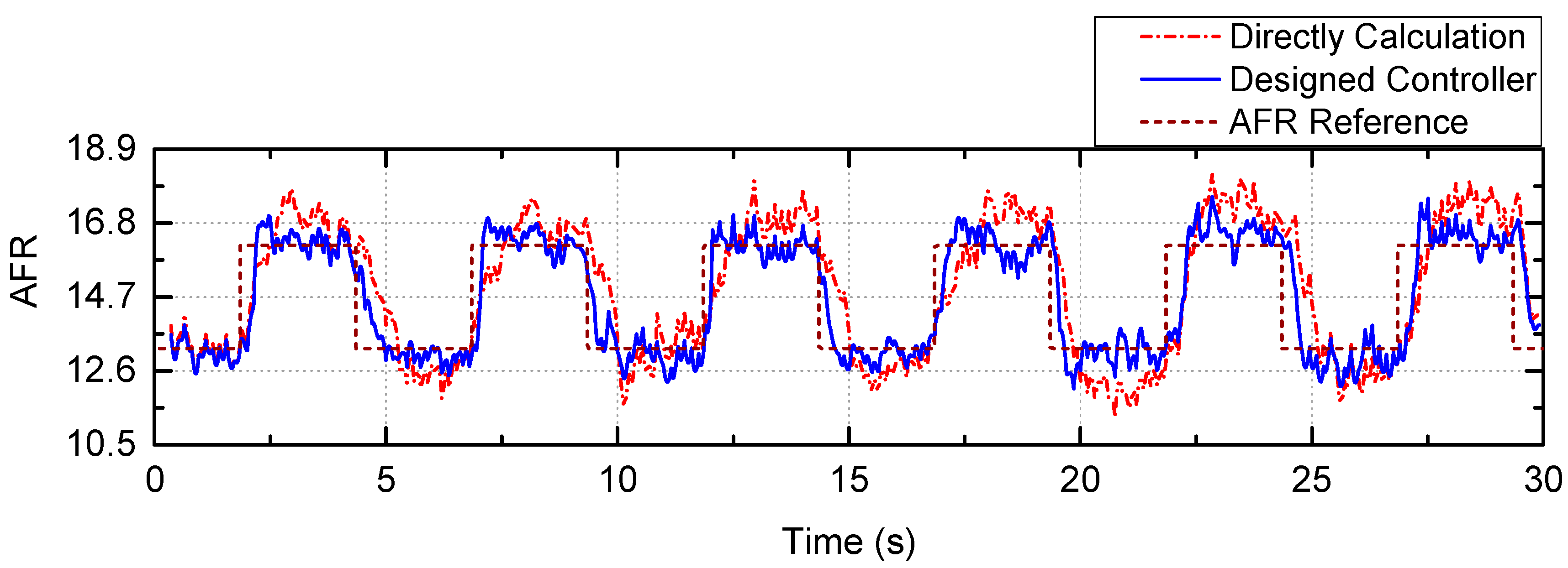
4. Simulation Validation

The system simulation validation was implemented in MATLAB Simulink based on the system structure in Figure 5. The AFR dynamic was used by the discrete time description in Equation (19) and k as the discrete iterations. To illustrate the effectiveness of the designed controller, the simulation was verified both at under steady and transient states.
Case 1: Steady state verification. The engine speed was held at 1200 RPM under the steady state, and the intake air mass was 15 g/s, and the relative parameters were τ e x h = 0.15 s , τ f = 2 s , and X = 0.7 . The sampling was once per working cycle. The controller was set at N = 6 , N u = 2 , γ = 0.02 , α = 0.7 , and the control object was taking the equivalence ratio output of ϕ e x h = 1 . The zero-mean, Gaussian white noise with a variance of 0.02 was added at the system output for the measurement noise. The simulation result is shown in Figure 6.
It could be found that the controlled input fuel injection was large at the beginning to accelerate the tracking of the referenced equivalence ratio objective. On the other hand, the variation of the controlled input indicated the effectiveness of the online parameter identification and the adaptive update control law.
Case 2: Transient state verification. In order to test the adaptive controller effectiveness, a simulation test with the parameter varying at different operation points was carried out. The engine speed and air mass parameters were obtained from the enDYNA engine simulation platform presented in our previous work [18]. The engine model parameters— X , τ f , τ e x h —were defined as the continuous variables in Figure 7 to simulate the uncertainty and sensor aging. The objected output was set as ϕ e x h = 1 . It should be noted here that based on the event-based sampling, the sampling time was changed by the engine speed. The total integration of the sampling time during this process was around 28 s.
The system output is shown in Figure 8. For the first part of the test process, the system output significantly varied because the online identification result dynamically approximated the actual value. Under the effect of system noise and parameter varying, the control output could be regulated near 1. It also could be found that at the 200th event, the engine load was increased and the gas mixture should become leaner as the fuel film evaporated, and at the 350th event, the engine load was decreased and the gas mixture became richer. The correlative output trends also can be found in Figure 8, and the adaptive controller regulated the system output back to the objective.
Based on the parameter settings, the relative model variables could be calculated using Equation (19). Online identification results of Equation (32) are shown in Figure 9. It could be concluded that the adaptive parameter identification had major fluctuations at the beginning because of the imprecise estimation, and the convergence with the parameter variation could be found. Using the GPC method, one could solve the control problem in the application of AFR regulation such as the unknown parameter and the uncertainty, time-delay, and time-varying. Consequently, the designed adaptive AFR controller displayed a noise suppression capability, as well as adaptive online prediction and self-correction on the SI engine system.

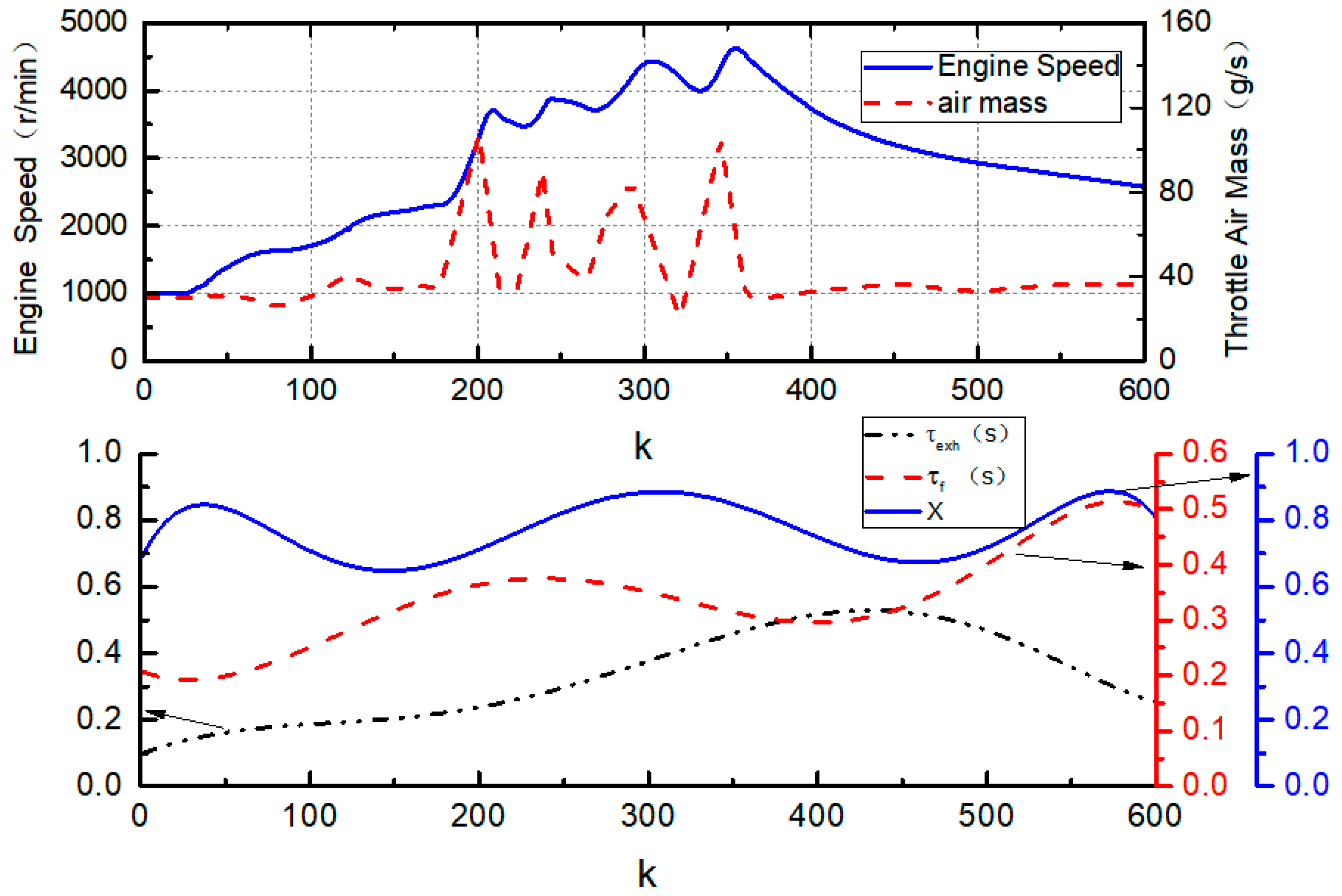
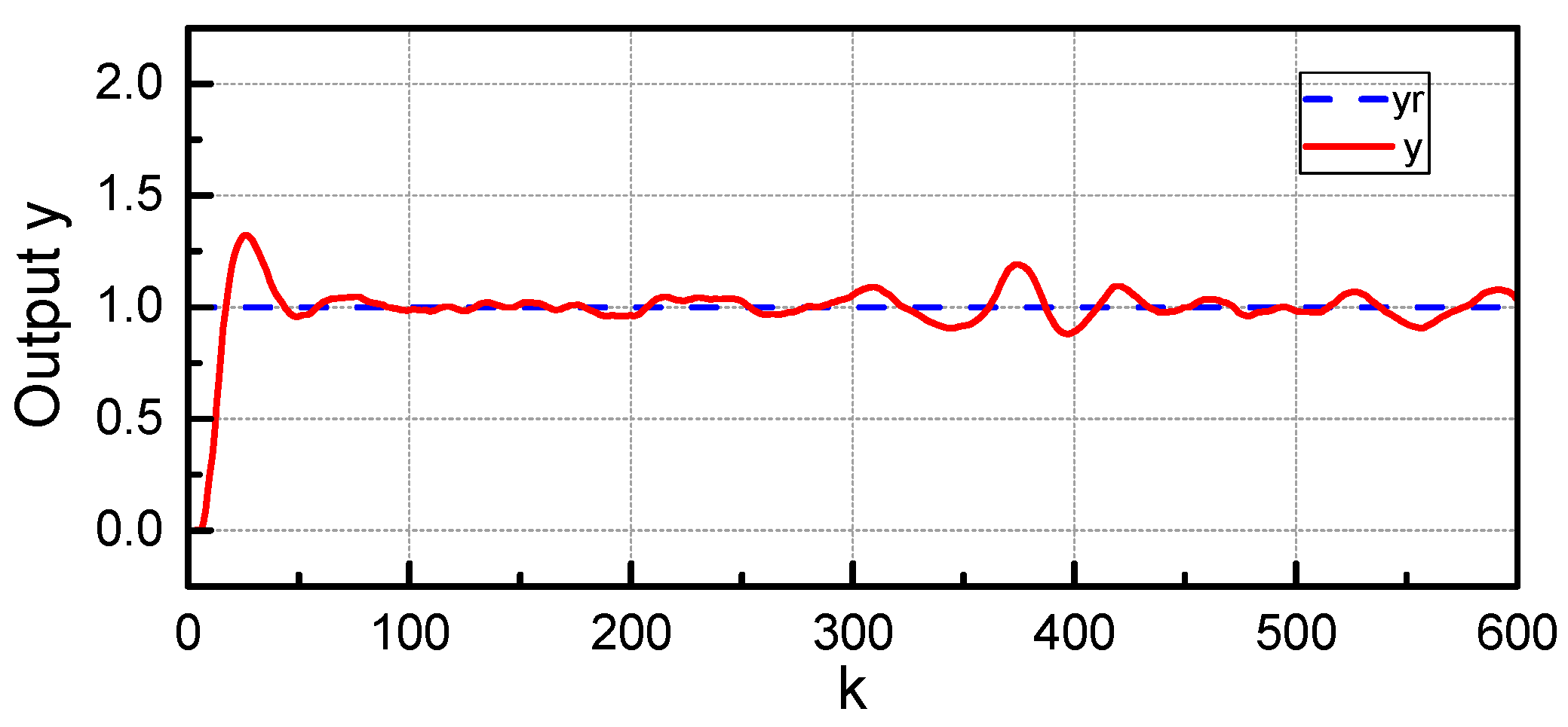
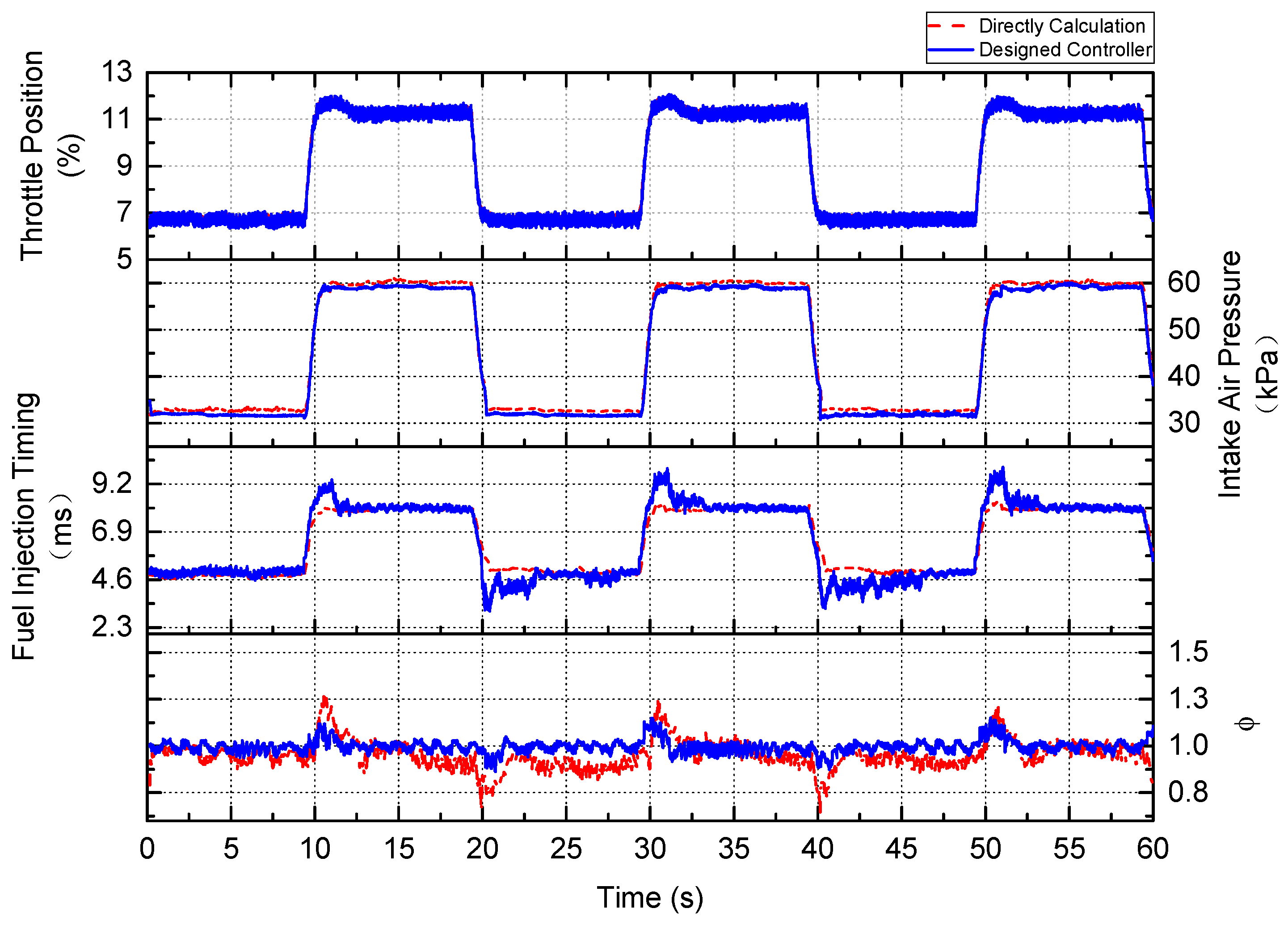
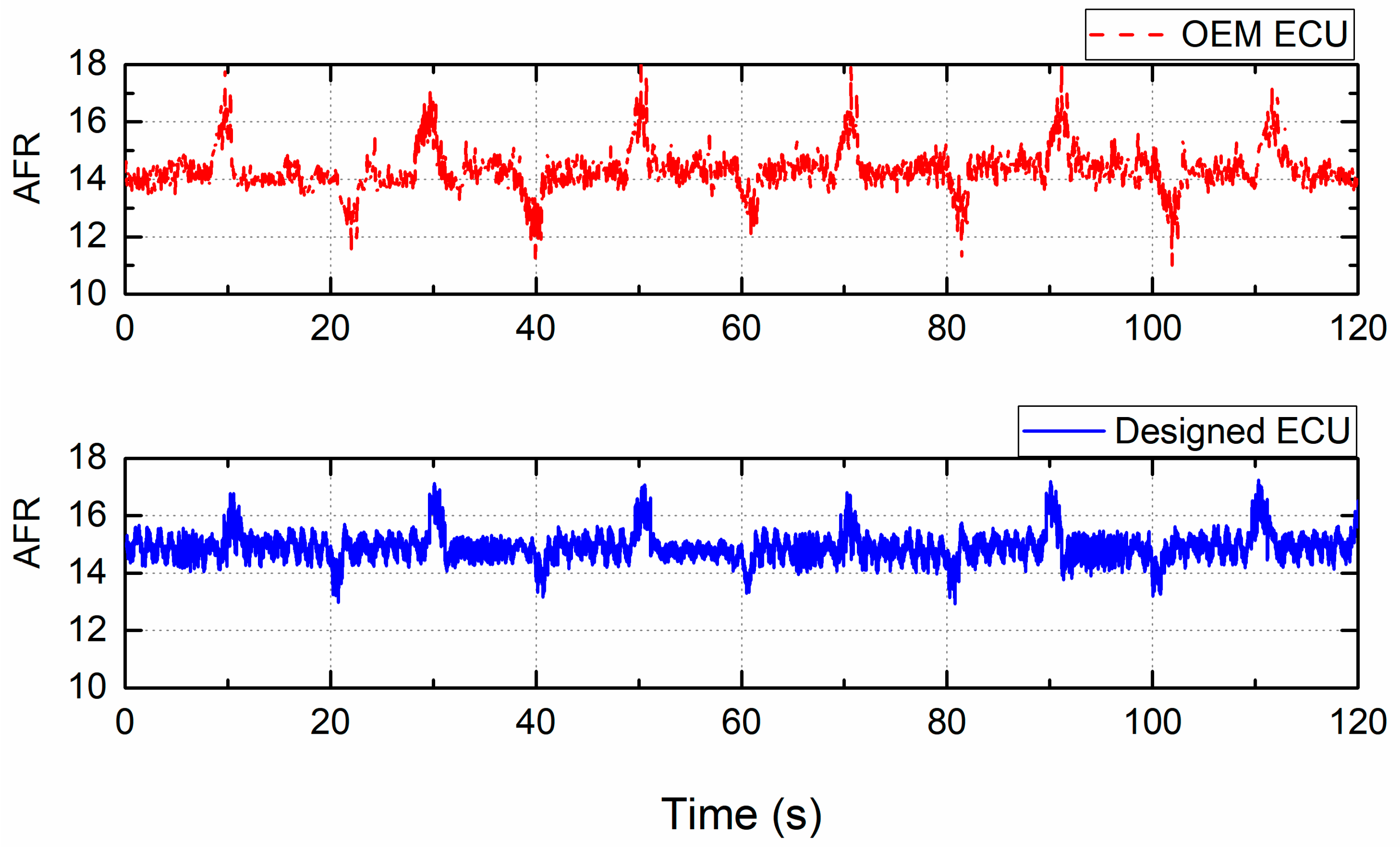
5. Experimental Implementation

The experimental validation of the controller design was conducted on an engine test bench installed with an OEM SGMW B15 engine. The geometry dimensions of the engine are listed in Table 1. Figure 10 shows the control system scheme of the engine test bench. The engine was connected with the MEBT-II dynamometer system. A BOSCH HFM5 MAF sensor was installed before the throttle plate. Before the TWC, an LC-2 UEGO sensor (Innovate Motorsports, Sycamore, IL, USA) was installed near the original HEGO sensor. The other necessary sensors and actuators for the engine control application, such as the MAP, temperature, position encoders, etc., were installed using the original OEM ones for the engine system. The engine ECU was implemented on a Freescale MC9S12XDP512 based controller, which was designed for the signal acquisition and control of the four-cylinder SI engine. The embedded software was generated by the model-based design method [25] in MATLAB Simulink. An ATI Vision-based calibration system was established for the control parameter online updating and internal data logging.
Three independent tests were designed for the proposed adaptive AFR controller verification. The engine was fueled with commercial gasoline and all the tests were conducted after the engine fully warmed-up with the coolant temperature around 70 °C.
Test 1: To validate the AFR control performance under load disturbance. The engine speed was restricted to 1500 rpm, and the throttle position was stepped, varying between 7% and 11% to simulate the transient load increase and decrease. The referenced equivalence ratio was one. The results of direct calculation of the fuel injection based on Equation (1) and the adaptive controller described in Figure 3 were compared to illustrate the effectiveness of the adaptive control.
In this test, the engine speed was constant and only the intake air mass changed to minimize the effort of the internal parameter varying. Figure 11 shows the results. It can be found that the fuel injection amount has the same trend with the intake air pressure in the direct calculation test. As the wall-wetting phenomenon existed, the exhaust equivalence ratio output overshoots when the throttle position was changed. The time-delay of the AFR dynamic variation can also be clearly seen. Comparably, the proposed adaptive AFR control method had the control compensation at the transient state to regulate the system output with the effect of the feedforward and feedback control. In the steady state, it also displayed a noise suppression capability.
Test 2: To compare the AFR regulation performance between the OEM ECU and the proposed controller in this work, the test condition was the same with Test 1. However, the internal parameter of the OEM ECU could not be directly acquired by the calibration system, therefore the exhaust AFR results were obtained by the installed UEGO sensor.
The comparable result is shown in Figure 12. On the OEM engine control system, the ECU controlled the exhaust equivalence ratio based on the HEGO sensor, which only had the switching signal representing the gas mixture lean or rich. The exhaust AFR obviously overshot when the throttle position changing. On the other hand, the proposed adaptive controller had the ability to overcome the time-delay in the system and had an advanced output. In addition, the noise could be suppressed to a reasonable level.
Test 3: To verify the response performance of the controller under the transient state, the dynamometer was set at 2000 rpm and the intake air pressure was adjusted to 70 kPa. Using the calibration system to switch the referenced AFR between 13.2 and 16.2, as well as a ±10% step change, the direct calculation method mentioned above and the proposed adaptive control scheme were compared.
Figure 13 shows the test results. Under these operation conditions, the engine was kept at the steady state to eliminate the effect of intake air mass observation and engine speed varying. Only the fuel injection calculation algorithm effected the test result. From the direct calculation method, the time-delay and AFR path dynamic characteristic could be clearly observed and the overshoot occurred at the referenced AFR objective stepping. It also clearly showed the modelling of the AFR path dynamics described in Section 2. Using the adaptive AFR regulation method based on the feedforward and feedback control, the transient overshoot and delay performance could be clearly improved compared with the direct calculation method. However, due to the parameter uncertainties, un-modelling error, measurement noise, and the error from the dynamometer system, the exhaust AFR also fluctuated at the fixed output reference.

6. Conclusions

An adaptive AFR controller design for the port-injected SI engine is presented in this work. To regulate the exhaust gas AFR at the reference value, the AFR path and SI engine dynamic modelling was implemented based on MVEM. The controller consisted of the fuel wall-wetting feedforward compensating controller and the adaptive feedback controller. All the control laws were conducted in the discrete domain using event-based sampling, and the parameters were obtained for an experimental engine system. A detailed analysis of the adaptive feedback controller design based on the generalized predictive control algorithms was introduced for the AFR regulation application to overcome the control problems such as the parameter varying and uncertainties, time-delay and nonlinearities, unknown dynamics and modelling error under complex working conditions. The simulation verification under steady and transient states was presented to demonstrate the effectiveness of the adaptive control law. Three comparative experiments were conducted on an engine test bench to validate the performance of the proposed AFR regulation controller design.
The simulation results showed that the proposed adaptive AFR control method was effective regarding noise suppression, online prediction, and self-correction on the SI engine system. The control algorithms could adaptively adjust the system input under different working conditions based on the iteration calculations to achieve a reasonable performance. Moreover, the experimental verification shows the effectiveness of the adaptive method for the AFR control application on the SI engine system. An acceptable performance compared with the OEM ECU results shows the potential usage of the generalized predictive control method to improve the feedback AFR control effect. Future work will involve studying the optimum control at different operating conditions and the combination of torque control based on the electronic throttle controlling.

Author Contributions

All authors have cooperated for the preparation of the work. Conceptualization, L.M. and C.Z.; Methodology, L.M.; Software and validation, L.M. and J.L.; Writing—Original Draft Preparation, L.M.; Writing—Review and Editing, J.L., X.W., and C.Z.

Funding

This material is based upon work supported by the supported by Fundamental Research Funds for the Central Universities (WUT: 2018IVA109). This work also supported by Nature Science Foundation of Hubei Province (2018CFB303).

Conflicts of Interest

The authors declare no conflict of interest.

Nomenclature

Symbol: DescriptionUnit
α : throttle position angle°
a 1 , a 2 , p 1 , p 2 , p n , p c : constant fitting parameters-
A F R s : stoichiometric air fuel ratio-
A F R : actual air fuel ratio-
e v : volumetric efficiency-
H u : fuel heating valueJ/kg
I : inertia of the engine and loadkg∙m2
m ˙ a p : air mass in the engine cylinderkg/s
m ˙ a t : air mass through the throttle platekg/s
m ˙ a t 1 : fitting constant-
m ˙ f c m d : injected fuel mass flow followed the control commandkg/s
m ˙ f c y l : fuel mass flow entering the cylinderkg/s
m ˙ f f : fuel mass flow of the wall film evaporationkg/s
m ˙ f v : fuel mass flow of the directly evaporationkg/s
m ˙ f c a l : calculated fuel mass amountkg/s
m ˙ f f c : fuel feedforward controller outputkg/s
X , X ^ : the fraction and its estimation value of the fuel flow into film -
τ f , τ ^ f : the fuel film evaporation time constant and its estimation value s
τ m : time constant of the gas mixings
τ o : time constant of the oxygen sensors
τ d : AFR transmission delays
τ e x h : time constant of the gas exhausting s
t i n j : time of the injector openingms
T i , T f , T l o a d : torque of indicated, friction and loadN∙m
T c , T e x h : time delay of the combustion and gas exhaustings
T : sampling times
T m a n , T a m b : temperature of the intake manifold and ambientK
n : engine speedr/min
p m a n : intake air pressurekPa
p a m b : ambient air pressurekPa
p c : pressure constant parameterkPa
p r : ratio of air pressure before and after the throttle-
η i : indicated efficiency -
R : gas constant J/(kg∙K)
ω : engine velocityrad/s
θ i : spark advance angle°
V m a n : volume of the intake manifoldL
λ : lambda, ratio of AFR and the stoichiometric ratio-
λ r e f : referenced lambda-
ϕ : fuel/air equivalence ratio-
ϕ c y l , ϕ e x h : fuel/air equivalence ratio in the cylinder and exhaust pipe-
N , N u : the maximum costing horizon and control horizon of GPC-
γ : control weighting in GPC-
c : delay step in GPC-
n a , n b : the order of the CARIMA model-

References

  1. Jiao, X.; Zhang, J.; Shen, T.; Kako, J. Adaptive air-fuel ratio control scheme and its experimental validations for port-injected spark ignition engines. Int. J. Adapt. Control 2015, 29, 41–63. [Google Scholar] [CrossRef]
  2. Shen, T.; Zhang, J.; Jiao, X.; Kang, M.; Kako, J.; Ohata, A. Transient Control of Gasoline Engines; CRC Press: Boca Ratonn, FL, USA, 2015. [Google Scholar]
  3. Wong, K.I.; Wong, P.K. Adaptive air-fuel ratio control of dual-injection engines under biofuel blends using extreme learning machine. Energy Convers. Manag. 2018, 165, 66–75. [Google Scholar] [CrossRef]
  4. Carbot-Rojas, D.A.; Escobar-Jiménez, R.F.; Gómez-Aguilar, J.F.; Téllez-Anguiano, A.C. A survey on modeling, biofuels, control and supervision systems applied in internal combustion engines. Renew. Sustain. Energy Rev. 2017, 73, 1070–1085. [Google Scholar] [CrossRef]
  5. Powell, J.D.; Fekete, N.P.; Chen-Fang, C. Observer-based air fuel ratio control. Control Syst. IEEE 1998, 18, 72–83. [Google Scholar] [CrossRef]
  6. Jensen, P.B.; Olsen, M.B.; Poulsen, J.; Hendricks, E.; Fons, M.; Jepsen, C. A New Family of Nonlinear Observers for SI Engine Air/Fuel Ratio Control; SAE Technical Paper 9706155. 1997. Available online: https://www.sae.org/publications/technical-papers/content/970615/ (accessed on 4 January 2019).
  7. Bresch-Pietri, D.; Chauvin, J.; Petit, N. Adaptive backstepping controller for uncertain systems with unknown input time-delay. Application to SI engines. In Proceedings of the 49th IEEE Conference on Decision and Control (CDC), Atlanta, GA, USA, 15–17 December 2010; pp. 3680–3687. [Google Scholar]
  8. White, A.; Guoming, Z.; Jongeun, C. Hardware-in-the-Loop Simulation of Robust Gain-Scheduling Control of Port-Fuel-Injection Processes. IEEE Trans. Control Syst. Technol. 2011, 19, 1433–1443. [Google Scholar] [CrossRef]
  9. Postma, M.; Nagamune, R. Air-Fuel Ratio Control of Spark Ignition Engines Using a Switching LPV Controller. IEEE Trans. Control Syst. Technol. 2012, 20, 1175–1187. [Google Scholar] [CrossRef]
  10. Pace, S.; Zhu, G.G. Sliding mode control of both air-to-fuel and fuel ratios for a dual-fuel internal combustion engine. J. Dyn. Syst. Measur. Control 2012, 134. [Google Scholar] [CrossRef]
  11. Wu, H.; Tafreshi, R. Fuzzy Sliding-mode Strategy for Air-fuel Ratio Control of Lean-burn Spark Ignition Engines. Asian J. Control 2018, 20, 149–158. [Google Scholar] [CrossRef]
  12. Kahveci, N.E.; Jankovic, M.J. Adaptive controller with delay compensation for Air-Fuel Ratio regulation in SI engines. In Proceedings of the American Control Conference (ACC), Baltimore, MD, USA, 30 June–2 July 2010; pp. 2236–2241. [Google Scholar]
  13. Kahveci, N.E.; Impram, S.T.; Genc, A.U. Adaptive Internal Model Control for Air-Fuel Ratio regulation. In Proceedings of the Intelligent Vehicles Symposium, Dearborn, MI, USA, 8–11 June 2014; pp. 1091–1096. [Google Scholar]
  14. Prucka, R.G.; Filipi, Z.S.; Hagena, J.R.; Assanis, D.N. Cycle-by-Cycle Air-to-Fuel Ratio Calculation During Transient Engine Operation Using Fast Response CO and CO2 Sensors. In Proceedings of the ASME 2012 Internal Combustion Engine Division Fall Technical Conference, Vancouver, BC, Canada, 23–26 September 2012; pp. 303–311. [Google Scholar]
  15. Hendricks, E. Engine Modelling for Control Applications: A Critical Survey. Meccanica 1997, 32, 387–396. [Google Scholar] [CrossRef]
  16. Guzzella, L.; Onder, C.H. Introduction to Modeling and Control of Internal Combustion Engine Systems; Springer: Berlin/Heidelberg, Germany, 2010; Volume 25, pp. 96–99. [Google Scholar]
  17. Hendricks, E.; Vesterholm, T. The Analysis of Mean Value SI Engine Models; SAE Technical Paper 920682. 1992. Available online: https://www.sae.org/publications/technical-papers/content/920682/ (accessed on 4 January 2019).
  18. Lei, M.; Zeng, C.; Hong, L.; Jie, L.; Wen, L.; Li, X. Research on Modeling and Simulation of SI Engine for AFR Control Application. Open Autom. Control Syst. J. 2014, 6, 803–812. [Google Scholar] [CrossRef]
  19. Hendricks, E.; Chevalier, A.; Jensen, M.; Sorenson, S.C.; Trumpy, D.; Asik, J. Modelling of the Intake Manifold Filling Dynamics; SAE Technical Paper 960037. 1996. Available online: https://www.sae.org/publications/technical-papers/content/960037/ (accessed on 4 January 2019).
  20. Hendricks, E.; Vesterholm, T.; Sorenson, S.C. Nonlinear, Closed Loop, SI Engine Control Observers; SAE Technical Paper 920237. 1992. Available online: https://www.sae.org/publications/technical-papers/content/920237/ (accessed on 4 January 2019).
  21. Kiencke, U.; Nielsen, L. Automotive Control Systems: For Engine, Driveline, and Vehicle; Springer: Berlin/Heidelberg, Germany, 2005; pp. 56–70. ISBN 978-3-540-26484-2. [Google Scholar]
  22. Clarke, D.W.; Mohtadi, C.; Tuffs, P.S. Generalized predictive control—Part I. The basic algorithm. Automatica 1987, 23, 137–148. [Google Scholar] [CrossRef]
  23. Wang, Z.; Zhu, Q.; Prucka, R. A Review of Spark-Ignition Engine Air Charge Estimation Methods; SAE Technical Paper 2016-01-0620. 2016. Available online: https://www.sae.org/publications/technical-papers/content/2016-01-0620/ (accessed on 4 January 2019).
  24. Hendricks, E.; Vesterholm, T.; Kaidantzis, P.; Rasmussen, P.; Jensen, M. Nonlinear Transient Fuel Film Compensation (NTFC); SAE Technical Paper 930767. 1993. Available online: https://www.sae.org/publications/technical-papers/content/930767/ (accessed on 4 January 2019).
  25. Vijayagopal, R.; Michaels, L.; Rousseau, A.P.; Halbach, S.; Shidore, N. Automated Model Based Design Process to Evaluate Advanced Component Technologies; SAE Technical Paper 2010-01-0936. 2010. Available online: https://www.sae.org/publications/technical-papers/content/2010-01-0936/ (accessed on 4 January 2019).
Figure 1. The structure of the AFR control system.
Energies 12 00173 g001
Figure 2. The schematic diagram of the dynamic AFR path.
Energies 12 00173 g002
Figure 3. The scheme of the adaptive controller.
Energies 12 00173 g003
Figure 4. The parameter identification result of X ^ and τ ^ f .
Energies 12 00173 g004
Figure 5. The feedback control scheme.
Energies 12 00173 g005
Figure 6. The simulation result of Case 1 (u as the fuel injection calculated by the controller, y as the engine equivalence ratio output).
Energies 12 00173 g006
Figure 7. Simulation parameters of Case 2. (Up) the measured engine parameters; (Down) the engine model parameters.
Energies 12 00173 g007
Figure 8. The simulation result of system output in Case 2 (yr as the referenced equivalence ratio, y as the engine equivalence ratio output).
Energies 12 00173 g008
Figure 9. The online identification result of the controller parameters (a1, a2, b1, and b2 as the parameters in Equation (32)).
Energies 12 00173 g009
Figure 10. The control system scheme of the engine test bench.
Energies 12 00173 g010
Figure 11. Experimental results of the control performance under load disturbance.
Energies 12 00173 g011
Figure 12. Comparison experimental results of the ECU controllers.
Energies 12 00173 g012
Figure 13. Experimental results of different control methods.
Energies 12 00173 g013
Table 1. SGMW B15 Engine Specifications.
Parameter TypeValue
Engine TypeSI,4 cylinders, In-line
Displacement (liters)1.485 L
Compression Ratio10.2:1
Bore (mm)74.7
Stroke (mm)84.7
Maximum torque146 N∙m/3600–4000 rpm
Maximum power82 kW/5800 rpm

