An Overall Bubble Diameter Model for the Flow Boiling and Numerical Analysis through Global Information Searching

Abstract

Bubble diameter is important for the three-dimensional nucleate boiling two-phase flow simulation. However, the bubble diameter is rarely considered as a variable because it is difficult to estimate. In this paper, a novel bubble diameter model is proposed for the boiling flow. The heat transfer growth, the breakup or coalescence of collision and the liquid impacting separation are considered as the factors affecting the bubble diameter, and three bubble diameter sub-models are developed to calculate the overall bubble diameter based on a departure diameter. In the model, the heat transfer growth is calculated after estimating the bubble location. The collision variation is deduced from the interfacial area concentration equation. The liquid impacting variation is calculated through phase interaction force and gas viscous force. The proposed model is conducted through global information searching in the flow boiling simulation and validated using the void fraction and temperature data from the literature. The effects of the heat transfer growth, the collision, and the separating volume on the bubble diameter are discussed.

1. Introduction

Nucleate boiling is a highly efficient heat transfer process due to the phase change latent heat transfer and the two-phase forced convection heat transfer in the near-wall region. It has been applied in many industrial facilities, such as nuclear reactor, chemical reactor, pipeline system for oil and gas transport and automotive industry [1].

An appropriate operating condition is the key to ensure the safety and the efficiency of the nucleate boiling technique. The gas–liquid flow with nucleate boiling is usually simulated through the Eulerian–Eulerian approach, in which the two phases are considered continuous, even though it should be a multiphase flow. However, the Eulerian–Eulerian approach is widely accepted and many multiphase interaction models are proposed based on it, such as the drag model, the wall boiling model and the inner-phase heat transfer model. High mass flux subcooled flow boiling was investigated by Kenarsari [2] through two-phase Eulerian numerical simulation and experimental study in horizontal micro-tubes. The effects of heat flux, mass flux, vapor quality, void fraction, and inlet subcooling on heat transfer characteristics are obtained and in a good agreement with the experimental results. Gao [3] introduced a wall heat flux partition algorithm in the water subcooled flow boiling simulation to decide the onset of the significant void, which is important for predicting the void fraction profile. Comparing with Bartolomei and Chanturiya’s experiment data [4] and Saha and Zuber’s [5] correlation, Gao’s work obtains a comparatively accurate liquid subcooling at the onset of the significant void.

Tu [6] pointed out that the bubble size correlation is essential for calculating the total rate of the interfacial momentum, energy and mass transport between the two phases in a low-pressure subcooled flow boiling. Due to the lack of experimental bubble size, the constant bubble diameter or the linear bubble diameter correlations [7,8] are usually used in the flow boiling simulations, which affects the simulation accuracy greatly. Anglart and Nylund [7] modeled the bubble diameter as a linear function of the local supercooling and the maximum bubble diameter in the near-wall region, which is validated only for relatively high-pressure flows. In Končar’s [8] research, a simple model of radial distribution of the bubble diameter is proposed, which introduces the exponent function of the local subcooling to describe the bubble diameter decrease due to the condensation in the subcooled flow field. Similarly, the model has a good agreement with the low pressure experimental data. Byong [9] also indicated that the bubble size is an importance factor for accurately predicting the subcooled flow boiling, adopted a volumetric conserved bubble size model and introduced new wall boiling and two-phase logarithmic wall function models. The volumetric conserved bubble size model proposed by the population balance equation [10] considers the breakup and the coalescence based on pre-assumed lognormal bubble size distribution. The benchmark calculation shows that the model can predict the high pressure experimental data fairly well. Colombo [11] also adopted the above model to predict the bubble diameter distribution, and employed the heat flux partitioning approach to establish a wall boiling model, which can provide relatively accurate Eulerian–Eulerian CFD (Computational Fluid Dynamics) predicted results except for the average bubble diameter and the mean velocity. Although the bubble size models can provide acceptable simulations, they are only verified partially in the subcooled flow boiling either in high pressure case or in low pressure case.

Focusing on the variation mechanism of the bubble diameter and its effect on the flow boiling simulation, a novel mathematical model of the bubble diameter is developed in this paper. The overall bubble diameter consists of the departure diameter (the initial diameter) and three terms contributed from the heat transfer growth, the collision and the fluid impact. On this basis, a two-phase Eulerian flow boiling simulation framework is proposed. Instead of using constant or temperature-dependent linear bubble diameter, multi-phase flow subcooled flow boiling simulation is carried out with consideration of the nonlinearity of bubble variation. The simulation approach is verified by experimental results from the literature. Then, a case study is carried out under different operating conditions.

2. Bubble Behavior in Flow Boiling

As shown in Figure 1, the flow domain is usually divided into two regions for the wall flow boiling: (Region 1) the near-wall region where the gas bubble generates, grows, slides and lifts up due to superheating temperature, and (Region 2) the main-flow region where the gas bubble flows following the liquid and condensing to transfer heat to the supercooled liquid.

In the flow boiling simulation, a constant bubble diameter or a linear correlation is easy to use, but it would be difficult to adequately describe the bubble size variation flow. After the bubble generation at the wall, the bubble size can be divided into three parts according to the bubble transformation manner. Under this consideration, the bubble departure diameter can be regarded as the initial bubble size. Phase change is the major manner changing the bubble size. Evaporation occurs in the near wall region, and condensation occurs in the subcooled liquid with mass transfer. The other two forms changing the bubble size can be seen in Figure 2. One is the collision that leads to coalescence or breakup, and the other is the crush because the liquid impact makes the phase interaction force exceed the maximum gas viscosity force. In multiphase simulation, the bubbles are usually equivalent to spheres and the equivalent diameter is to describe the bubble size.

3. Bubble Diameter Model

The bubble diameter, d_b, is defined as follows:

$$d_b=f(d_d,d_{heat},d_{collision},V)$$

(1)

where $d_d$ is the bubble departure diameter taken as the initial size of the bubble, $d_{heat}$ is the bubble size variation contribution due to the heat transfer, $d_{collision}$ is the bubble size variation contribution due to the collision, and $V$ is the separating volume function representing the bubble size variation due to the phase interaction force.

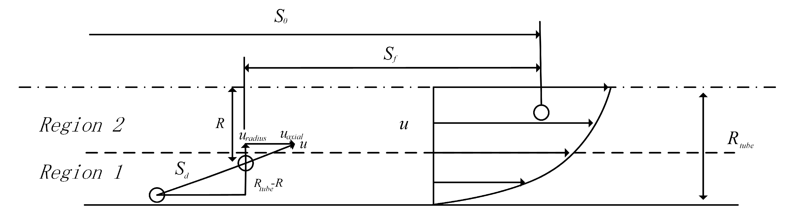
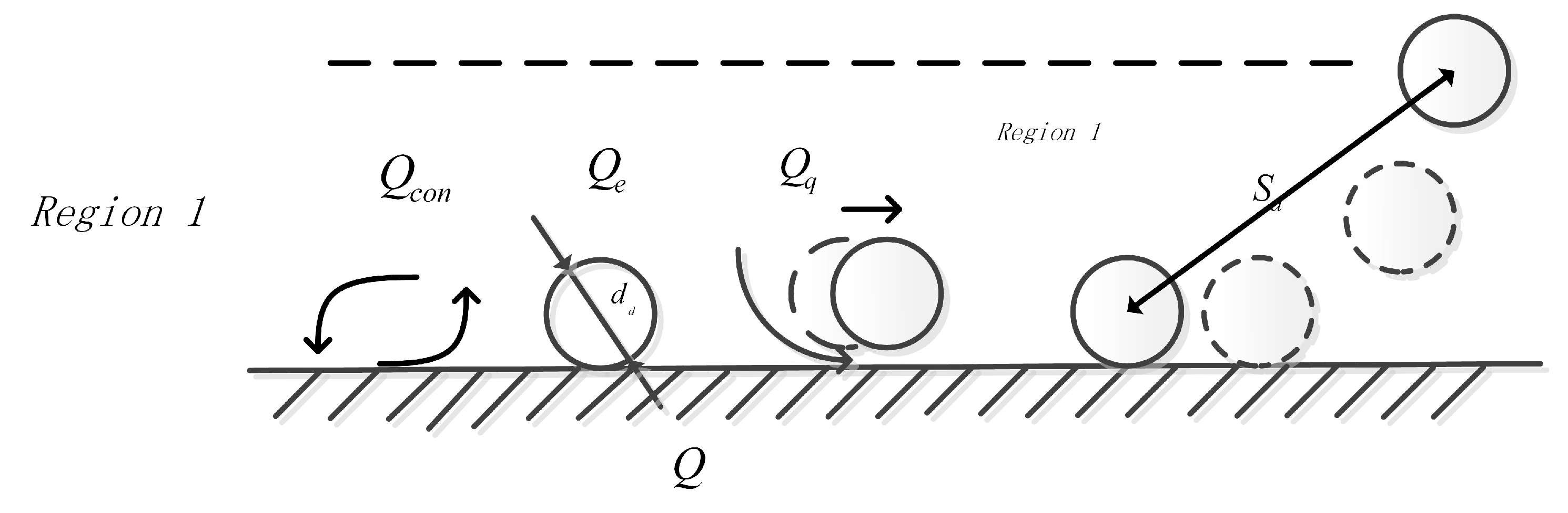
3.1. Bubble Departure Diameter

For the critical situation of bubble departure, many correlations [12,13,14,15] have been presented by deriving the force equilibrium equation including the surface tension force, the drag force, the buoyancy force, the lift force, etc. Some modifications [16,17,18] have also been done considering the heat transfer effect through the Jacob number and the contact angle. According to the lumped energy balance during the bubble growth and lift up process, correlations [19,20,21] of the bubble departure diameter are proposed as functions of the pressure, the saturation temperature and latent heat in a superheated liquid. Although some of them achieve good predictions in the bubble departure diameter, they are more proper for the pool boiling case rather than the flow boiling case. Comparing with the models mentioned above, the Tolubinsky model [22] is more appropriate for the flow boiling [1,3,23], which is given as follows

$$d_d=\min \left(0.0014,0.0006e^{-\frac{\Delta T_w}{45}}\right)$$

(2)

where $\Delta T_w$ is the temperature difference between the wall and the liquid.

3.2. Bubble Size Due to Heat Transfer

In the subcooled flow boiling, the temperature of gas or liquid varies with time and depends on the bubble flow route. The changing temperature leads to a varying heat transfer growth rate of the bubble. To calculate the bubble heat transfer growth rate, two key variables should be given: (1) the temperature variation; and (2) the capacity of bubble growth rate. The relation between the heat transfer growth rate and the temperature difference is established based on Zuber’s model [19]. The bubble is assumed to be a sphere considering the two-way heat transfer from the liquid thermal boundary layer to the bubble and the cooler liquid in the stabilized supersaturated temperature environment,

$$r_b=\frac{2}{\pi }\frac{{\rho }_l{C}_{p,l}\Delta T}{{\rho }_g{h}_{lg}}\left(1-\frac{q_b\sqrt{\pi {\alpha }_{l}t}}{2k_l\Delta T}\right)\sqrt{\pi {\alpha }_{l}t}$$

(3)

where t is the time of heat transfer, $k_l$ is the heat conductivity, $q_b$ is the heat transfer from the liquid thermal boundary layer to the liquid. Especially, $q_b$ equals zero in the constant liquid temperature field. Based on the constant fluid property assumption, the bubble size increases if the temperature difference is positive and vice versa. In the model, the environment temperature is uniform and the heat transfers are the same in different directions. To take into account the nonuniformity of the environment temperature, an approximate average heat loss of 50% from the total is used. The bubble diameter growth rate due to heat transfer can be calculated as

$$d_{heat}=\frac{2}{\sqrt{\pi }}\frac{{\rho }_l{C}_{p,l}}{{\rho }_g{h}_{fg}}\sqrt{\frac{k}{{\rho }_l{C}_{p,l}}}\Delta T\sqrt{t}$$

(4)

The Eulerian–Eulerian multiphase simulation cannot identify the bubble route, so the temperature difference and the square root of time are not available. An approximate method for the temperature difference and the time is applied in this paper to solve the problem. A variable n is introduced as the ratio between the flow distance S and the unit distance dS.

$$n=\frac{S}{\mathrm{d}S}$$

(5)

Then, the average temperature difference can be obtained

$$\Delta T=T_{wl}-T_{wg}+\frac{(T_l-T_g)-(T_{wl}-T_{wg})}{n}\mathrm{for}\mathrm{the}\mathrm{near}-\mathrm{wall}\mathrm{region}\left(\mathrm{region}1\right)$$

(6)

$$\Delta T=\frac{(T_l-T_g)}{n}\mathrm{for}\mathrm{the}\mathrm{main}-\mathrm{flow}\mathrm{region}\left(\mathrm{region}2\right)$$

(7)

where $T_{wl}$ and $T_{wg}$ are the liquid and gas temperatures at the wall, and $T_l$ and $T_g$ are the liquid and gas temperatures in the main flow. The temperature difference of the near-wall region is the sum of the initial temperature difference and the average temperature variation. In the main-flow region, the bubble enters the single phase flow as an external object, so the initial temperature difference is zero and only the average temperature variation is considered. The liquid or gas temperature will be replaced by the saturation temperature $T_{sat}$ considering the unsaturation heat transfer.

The time term can be calculated by

$$\sqrt{t}=n\sqrt{\frac{\mathrm{d}S}{u_g}}=\frac{S}{\sqrt{\mathrm{d}S\times u_g}}$$

(8)

where $S$ is the flow distance, and $u_g$ is the velocity. The flow distance $S$ is a function of location consisted of two parts, the departure and departure-lifting distance $S_d$ and the flow distance $S_f$, as shown in Figure 1.

Because of the complexity of the flow boiling, the criterion of the bubble merging with the main flow is difficult to determine exactly. In this work, the liquid velocity is used as a simplified criterion to distinguish whether the bubble has left the near-wall region. In the near-wall region, the bubble path is the syntheses of the radial and axial distances. In the main-flow region, the bubble path is simplified as the mean axial distance without disturbances. Thus, the flow distance S can be calculated as

$$S=S_d,S_d\approx (R_{tube}-R){\left(\frac{u_l}{u_{l,\mathrm{radial}}}\right)}^2,u_l<C\times u_{l,\max }\mathrm{for}\mathrm{the}\mathrm{near}-\mathrm{wall}\mathrm{region}\left(\mathrm{region}1\right)$$

(9)

$$S=S_d+S_f,S_f\approx \frac{1}{2}\times (S_0-S_d),u_l\ge C\times u_{l,\max }\mathrm{for}\mathrm{the}\mathrm{main}-\mathrm{flow}\mathrm{region}\left(\mathrm{region}2\right)$$

(10)

where $R$ is the pivot distance, $R_{tube}$ is the tube radius, $S_0$ is the axial distance from inlet, $u_{l,\max }$ is the liquid phase main stream velocity, and $C$ is the bubble location factor.

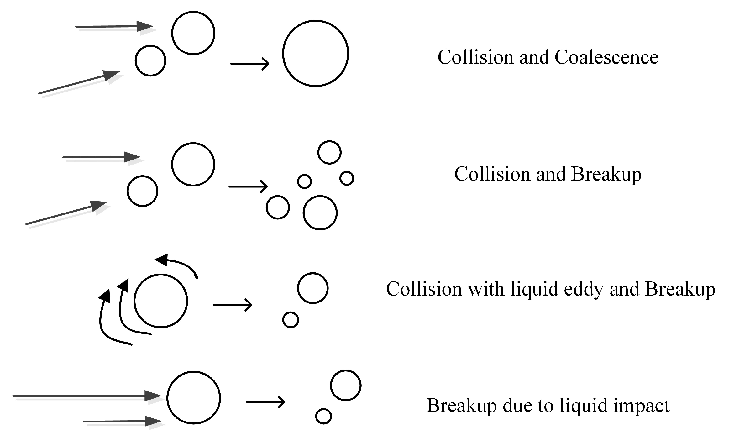
3.3. Bubble Size Due to Collision

The contributions of bubble collision coalescence and breakup are extracted from the interfacial area concentration and Hibiki [24] research. The bubble coalescence rate and the bubble breakup rate can be described in an interfacial area concentration transport equation [24] as follows,

$$\frac{\partial a_i}{\partial t}+\nabla \times a_i{u}_{iac}={\displaystyle \sum {\varphi }_{bc}+{\varphi }_{phase}}+{\varphi }_{pressure}$$

(11)

where ${\varphi }_{bc}$ is the changing rate of the interfacial area concentration due to bubble breakup or coalescence, ${\varphi }_{phase}$ is that due to phase change, and ${\varphi }_{pressure}$ is that due to pressure change.

In the case of only considering the breakup or coalescence due to collision, the last two terms on the right hand side of Equation (11) can be neglected. Then, it becomes

$$\frac{\partial a_i}{\partial t}+\nabla \times a_i{u}_{iac}={\displaystyle \sum {\varphi }_{bc}}=-{\varphi }_{RC}+{\varphi }_{TI}$$

(12)

where ${\varphi }_{RC}$ is the bubble coalescence rate and ${\varphi }_{TI}$ is the bubble breakup rate, which can be given as [24]:

$${\varphi }_{RC}=\frac{1}{3\psi }{\left(\frac{\alpha }{a_i}\right)}^2{f}_C{n}_b{\lambda }_C$$

(13)

$${\varphi }_{TI}=\frac{1}{3\psi }{\left(\frac{\alpha }{a_i}\right)}^2{f}_B{n}_e{\lambda }_B$$

(14)

where $f_C$ is the bubble random collision frequency, $f_B$ is the bubble eddy random collision frequency, ${\lambda }_C$ is the coalescence efficiency due to bubble random collision induced by turbulence in liquid phase, and ${\lambda }_B$ is the breakup efficiency due to collision of the turbulent eddy with the bubble. The collision and break up are ignored due to low rigidity.

$$f_C=\frac{{\gamma }_C^{\text{'}}\alpha {\epsilon }^{1/3}}{d_b^{2/3}\left({\alpha }_{\max }-\alpha \right)}$$

(15)

$$f_B=\frac{{\gamma }_B^{\text{'}}\alpha {\epsilon }^{1/3}}{d_b^{2/3}\left({\alpha }_{\max }-\alpha \right)}$$

(16)

$${\lambda }_C=\exp \left(-K_C\sqrt[6]{\frac{d_b^5{\rho }_f^3{\epsilon }^2}{{\sigma }^3}}\right)$$

(17)

$${\lambda }_B=\exp \left(-K_B\times \frac{\sigma }{{\rho }_f{d}_b^{5/3}{\epsilon }^{2/3}}\right)$$

(18)

where Kc is 1.29 and K_B is 1.37 [24]. The bubble diameter is considered as the variable in the transport equation, and the influence of bubble collision is represented by the interface concentration variation. It accurately represents the change of the interfacial area concentration but ignores the change of the bubble diameter itself. Interfacial area concentration is the interfacial area between two phases of per unit mixture volume. To calculated bubble collision, the interfacial area concentration is calculated in algebra by the Particle model which is derived from the surface area to volume ratio [3,25],

$$a_i=\frac{\alpha \times \pi d_b{}^2}{\frac{1}{6}\pi d_b{}^3}=\frac{6\alpha }{d_b}$$

(19)

Through Equation (19), the collision effect is considered in the bubble diameter calculation directly. When $a_i$ is replaced by $d_b$ and only the time gradient is considered, the contributions of coalescence and breakup mechanisms by collision to the averaged bubble size variations can be obtained:

$$d_{collision}=\frac{1}{216}(\frac{0.188\alpha {\epsilon }^{1/3}{d}_b{}^{1/3}}{{\alpha }_{\max }-\alpha }{\lambda }_C-\frac{0.264(1-\alpha ){\epsilon }^{1/3}{d}_b{}^{1/3}}{{\alpha }_{\max }-\alpha }{\lambda }_B)\mathrm{d}t\times \frac{n}{2}$$

(20)

where n/2 is introduced to consider the average distance from 0 to n times of unit distance, $\mathrm{d}t=\mathrm{d}S/u_g$ is the unit time.

3.4. Bubble Size Due to Phase Interaction Force

If the external force difference $\Delta F$ exceeds the viscosity force and the deformation reaches the critical size, the bubble will break up because the intermolecular forces cannot maintain the bubble shape anymore, and the external force difference has a similar tearing effect on the bubble. In the flow boiling, the external force is mainly caused by the liquid impact and can be calculated by the drag force difference. Assuming the separating gas velocity is equal to the liquid velocity, the separating volume function can be derived by the momentum theorem (the force on a particle is equal to the rate of change of momentum of that particle) as follows

$$V=\frac{\mathrm{grad}(F)\times \mathrm{d}S-F_{vis}}{{\rho }_g\Delta u}t\approx \frac{\mathrm{Max}(\Delta F)-F_{vis}}{{\rho }_g\Delta u}$$

(21)

where $\Delta u$ is the relative velocity between liquid and gas, $F_{vis}$ is the bubble viscous force, grad(F) is the gradient of phase interaction force, and $\Delta F$ is calculated by the phase interaction force difference of two adjacent units. Equation (20) considers the eddies influence to supplement Equation (21) which cannot consider the liquid cutting effect in different directions.

3.5. Overall Bubble Diameter and Information Searching

The overall bubble diameter can be described as follows,

$$d_b=\sqrt[3]{{(d_d+d_{heat}+d_{collision})}^3-\frac{6}{\pi }V}$$

(22)

where d_b is deduced by the bubble volume.

The bubble diameter model is compiled in Fluent software through C language. The calculation frame consists of four parts, as shown in Figure 3: the blue route is for the bubble departure diameter, the red route is for the heat transfer bubble size contribution, the yellow route is for the collision bubble size contribution and the green route is for the separating volume. Information of general multi-phase flow is not sufficient for the proposed new bubble diameter model. As a result, adding some data from the whole flow field into the computation is essential in the calculation, which tightly connects the computation variables and the flow condition together. The information searching scheme can be thought as a reform of the computation element regarding the data collection. Firstly, the main flow velocity is needed to determine the element location in the flow, for which only nearby elements are enough. Given as Loop 1, the calculated range is obtained according to the distance in the flow direction under the first global search, and the element velocities in the range are compared to fix the location. The second information searched is the temperature difference at the wall for determining the initial temperature. Seen as Loop 2, boundary elements nearby the presented element determined by the second global search are used to average the wall temperature. The phase interaction force difference $\Delta F$ between elements is the third information needed to represent the tear force of liquid impact. In Loop 3, a series of subtractions are done using the phase interaction forces of neighbor elements determined by the third global search to obtain the maximum force difference. Another global searching task over logic level of the three loops searching is conducted before every iteration of the computation to allocate information to the computation elements. In other words, information searching and allocating are the cores of the present computation apart from solving the multi-phase equations and the turbulence equations.

4. Flow Boiling Model Schemes

4.1. Gas–Liquid Two Phase Flow Conservation Equation

The continuity equation for phase q:

$$\frac{\partial }{\partial t}\left({\alpha }_q{\rho }_q\right)+\nabla \left({\alpha }_q{\rho }_q{\overrightarrow{u}}_q\right)={\displaystyle \sum _{p=1}^n\left({\dot{m}}_{pq}-{\dot{m}}_{qp}\right)}+S_q$$

(23)

The momentum equation for phase q:

$$\frac{\partial }{\partial t}\left({\alpha }_q{\rho }_q{\overrightarrow{u}}_q\right)+\nabla \left({\alpha }_q{\rho }_q{\overrightarrow{u}}_q{\overrightarrow{u}}_q\right)=-{\alpha }_q\nabla p+\nabla {\tau }_q+{\alpha }_q{\rho }_q\overrightarrow{g}+{\displaystyle \sum _{p=1}^n\left({\dot{m}}_{pq}{\overrightarrow{u}}_{pq}-{\dot{m}}_{qp}{\overrightarrow{u}}_{qp}\right)}+{\displaystyle \sum \overrightarrow{F}}$$

(24)

The energy equation for phase q:

$$\frac{\partial }{\partial t}\left({\alpha }_q{\rho }_q{h}_q\right)+\nabla \left({\alpha }_q{\rho }_q{\overrightarrow{u}}_q{h}_q\right)=-{\alpha }_q\frac{\partial p_q}{\partial t}+{\tau }_q:\nabla {\overrightarrow{u}}_q-\nabla {\overrightarrow{q}}_q+S_{source,q}+{\displaystyle \sum _{p=1}^n\left(Q_{pq}+{\dot{m}}_{pq}{h}_{pq}-{\dot{m}}_{qp}{h}_{qp}\right)}$$

(25)

4.2. Inner-Phase Mass Transfer and Heat Transfer

In the interior of the flow, the mass transfer rate between the two phases depends upon the temperature of the liquid and the gas, the interphase heat transfer coefficient and the latent heat. The temperature affects the mass transfer direction. The mass transfer rate $\dot{m}$ is

$$\dot{m}=\frac{Q-Q_T}{h_{\lg }}=\frac{h_{inter}{a}_i\left(T_{sat}-T_l\right)}{h_{\lg }}$$

(26)

where $a_i$ is the interfacial area concentration and can be calculated by Equation (19). The interfacial heat transfer coefficient $h_{inter}$ is modeled by Ranz–Marshall [26] correlation,

$$Nu=2.0+0.6{\mathrm{Re}}_p^{0.5}{\mathrm{Pr}}^{1/3}$$

(27)

where Re_p is the relative Reynolds number regarding the diameter of the p phase and the relative velocity and Pr is the Prandtl number of the q phase.

4.3. Wall Boiling Model

The manners of the wall boiling heat transfer include the liquid convection heat transfer, the gas convection heat transfer, the latent heat transfer by liquid evaporation, and the quench heat transfer, as shown in Figure 4. The gas convection is not obvious when the gas bubble is little. The quench heat transfer is resulted by the liquid and wall contact and the gas and wall contact successively. The wall boiling heat equation is

$$Q_w=Q_{con}+Q_e+Q_q$$

(28)

where $Q_w$ is the total heat flux, $Q_{con}$ is the convective heat flux, and $Q_e$ is the gas evaporation latent heat flux. In fact, the bubble nucleation starts at the wall due to the local overheating caused by the wall roughness or other factors. The bubble keeps growing for phase exchange and heat expansion until it departs from the wall for force equilibrium.

Usually, the bubble departure diameter, the bubble departure frequency and the nucleation site density are used to describe the wall heat transfer. Thus, the heat flux can be given as

$$Q_{con}=h_{con}\left(T_w-T_l\right)\left(1-A_b\right)$$

(29)

$$Q_e=m_b{N}_w{h}_{lg}$$

(30)

$$Q_q=\frac{2k_l\sqrt{f}}{\sqrt{\pi {\lambda }_l}}\left(T_w-T_l\right)$$

(31)

where $h_{con}$ is the convection heat transfer coefficient between the liquid and the wall, $A_b$ is the wall surface covered by gas, $\left(1-A_b\right)$ is the wall surface covered by liquid, $m_b$ is the bubble mass regarding the bubble departure diameter, $N_w$ is the nucleation site density, and $f$ is the bubble departure frequency. The wall surface covered by gas, $A_b$, is a function of the bubble departure diameter, $d_d$, and the nucleation sites density, $N_w$, as follows

$$\{\begin{array}{c}\begin{array}{l}{A}_b=K\frac{N_w\pi d_d^2}{4}\\ \end{array}\\ K=4.8e^{\left(-\frac{Ja}{80}\right)}\end{array}$$

(32)

where K is the empirical constant calculated by Del Valle and Kenning correlation [27] and Ja is the Jakob number.

The bubble departure frequency is [28]

$$f=\sqrt{\frac{4g\left({\rho }_l-{\rho }_g\right)}{3{\rho }_l{d}_d}}$$

(33)

The Nucleation site density is [29]

$$N_w={210}^{1.805}{\left(T_w-T_{sat}\right)}^{1.805}.$$

(34)

4.4. Interphase Momentum Transfer

The velocity of each phase changes with the phase interaction force through the momentum exchange. The phase interaction force $\overrightarrow{F}$ [25,30] is

$${\displaystyle \sum \overrightarrow{F}}={\overrightarrow{F}}_{lift}+{\overrightarrow{F}}_{vm}+{\overrightarrow{F}}_{TD}+{\overrightarrow{F}}_{WL}+{\overrightarrow{F}}_{drag}$$

(35)

where ${\overrightarrow{F}}_{lift}$ is the lift force acted on a particle, droplet or bubble mainly due to velocity gradients in the primary-phase flow field, ${\overrightarrow{F}}_{vm}$ is the virtual mass force that occurs when a secondary phase accelerates relative to the primary phase, ${\overrightarrow{F}}_{TD}$ is the turbulent dispersion force that acts as a turbulent diffusion in the dispersed flow accounting for the interphase turbulent momentum transfer, ${\overrightarrow{F}}_{WL}$ is the wall lubrication force that acts in the lateral direction and tends to push the secondary phases away from the wall, and ${\overrightarrow{F}}_{drag}$ is the drag force aroused by the interfacial friction force and pressure differences that acts on the vapor bubble. Among these interphase forces, the drag force, ${\overrightarrow{F}}_{drag}$, is the dominant component.

The drag force per unit volume can be expressed as [25,30]

$$F_{drag}=0.75\frac{{\alpha }_g{\rho }_l{C}_D\Delta u^2}{d_{\mathrm{b}}}$$

(36)

where $\Delta u$ is the relative velocity between the liquid and the gas, and $C_D$ is the drag force coefficient that can be given as [31]

$$\{\begin{array}{l}{C}_D=24\left(1+0.15{\mathrm{Re}}^{0.687}\right)/\mathrm{Re}\mathrm{Re}\le 1000\\ C_D=0.44\mathrm{Re}>1000\end{array}$$

(37)

The lift force can be calculated as follows [25,30]

$${\overrightarrow{F}}_{lift,q}=-C_{lift}{\alpha }_q\left({\overrightarrow{u}}_q-{\overrightarrow{u}}_p\right)\times \left(\nabla \times {\overrightarrow{u}}_q\right)$$

(38)

where C_lift is lift force coefficient that can be calculated [32].

$$C_l=\{\begin{array}{l}0.0767\phi \le 6000\\ -\left(-0.12-0.2e^{-\frac{\phi }{3.6}\times {10}^{-5}}\right)e^{\frac{\phi }{3}\times {10}^{-7}}6000<\phi <5\times {10}^7\\ -0.6353\phi \ge 5\times {10}^7\end{array},\phi ={\mathrm{Re}}_p{\mathrm{Re}}_w$$

(39)

$${\mathrm{Re}}_p=\frac{{\rho }_q^{}\left|{\overrightarrow{u}}_q-{\overrightarrow{u}}_p\right|d_p^{}}{{\mu }_q^{}}$$

$${\mathrm{Re}}_w=\frac{{\rho }_q^{}\left|\nabla \times {\overrightarrow{u}}_q\right|d_p^{}}{{\mu }_q^{}}$$

The virtual mass force can be obtained [25,30]

$${\overrightarrow{F}}_{vm,q}={\alpha }_q{\rho }_p{C}_{vm}\left(\frac{d{\overrightarrow{u}}_q}{dt}-\frac{d{\overrightarrow{u}}_p}{dt}\right)$$

(40)

where $C_{vm}$ is the virtual mass force coefficient and given as 0.5.

The wall lubrication force is [25,30]

$${\overrightarrow{F}}_{WL}=C_{WL}{\rho }_q{\alpha }_q{\left|{\overrightarrow{u}}_q-{\overrightarrow{u}}_p\right|}^2{\overrightarrow{n}}_w$$

(41)

where $C_{WL}$ is the wall lubrication force coefficient [33].

$$C_{WL}=\max \left(0,\frac{-0.001}{d_b}+\frac{0.05}{y_w}\right)$$

(42)

where $y_w$ is the distance to the nearest wall.

The turbulent dispersion force is [25,30]

$$F_{TD}=C_{TD}\frac{3{\alpha }_q{\rho }_p{C}_D\Delta u^2}{4d_b}\frac{{\mu }_{tq}}{{\delta }_{pq}{\rho }_q}\left(\frac{\nabla {\alpha }_q}{{\alpha }_q}-\frac{\nabla {\alpha }_p}{{\alpha }_p}\right)$$

(43)

where $C_{TD}=1$ is the turbulent dispersion force coefficient [34].

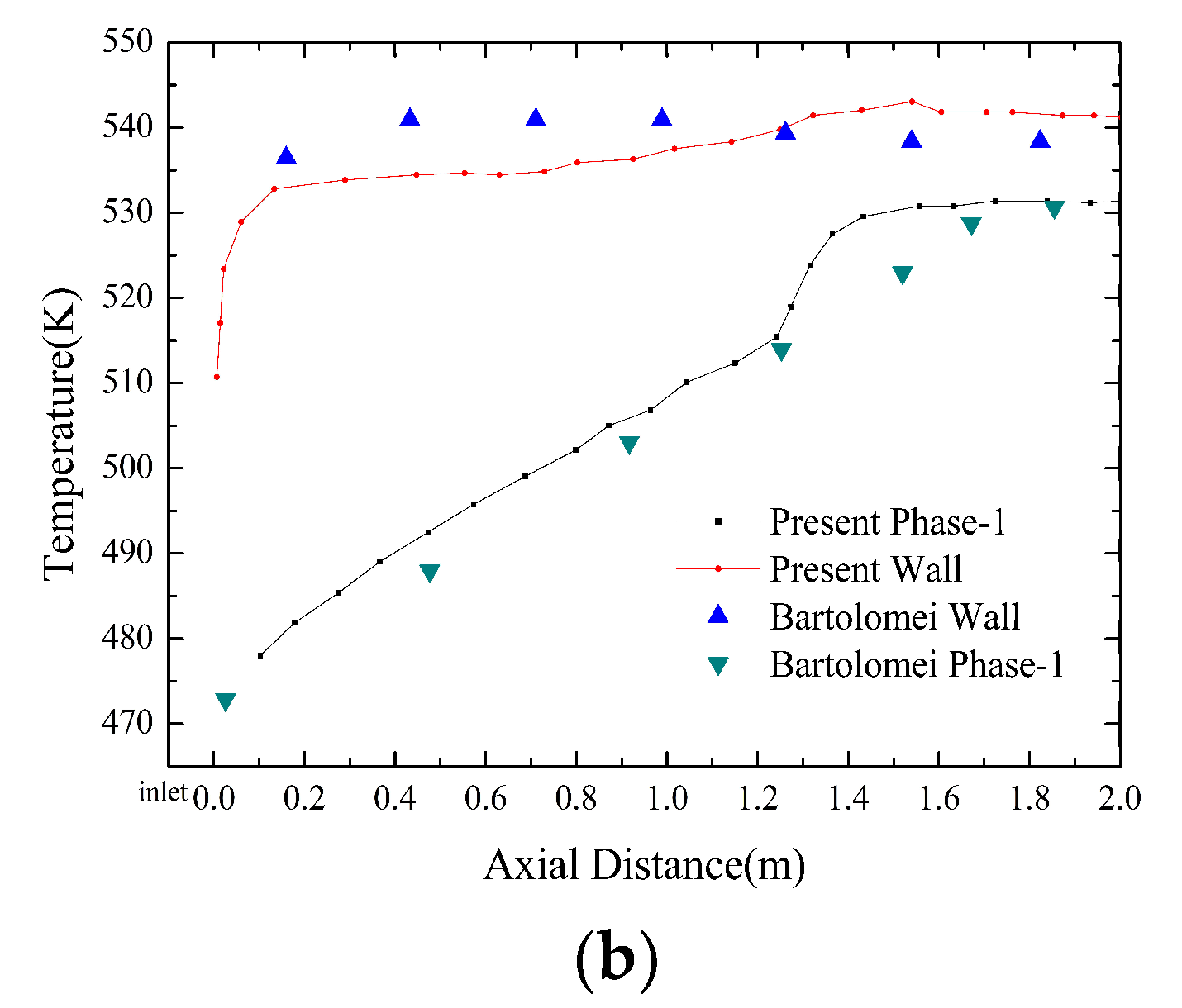
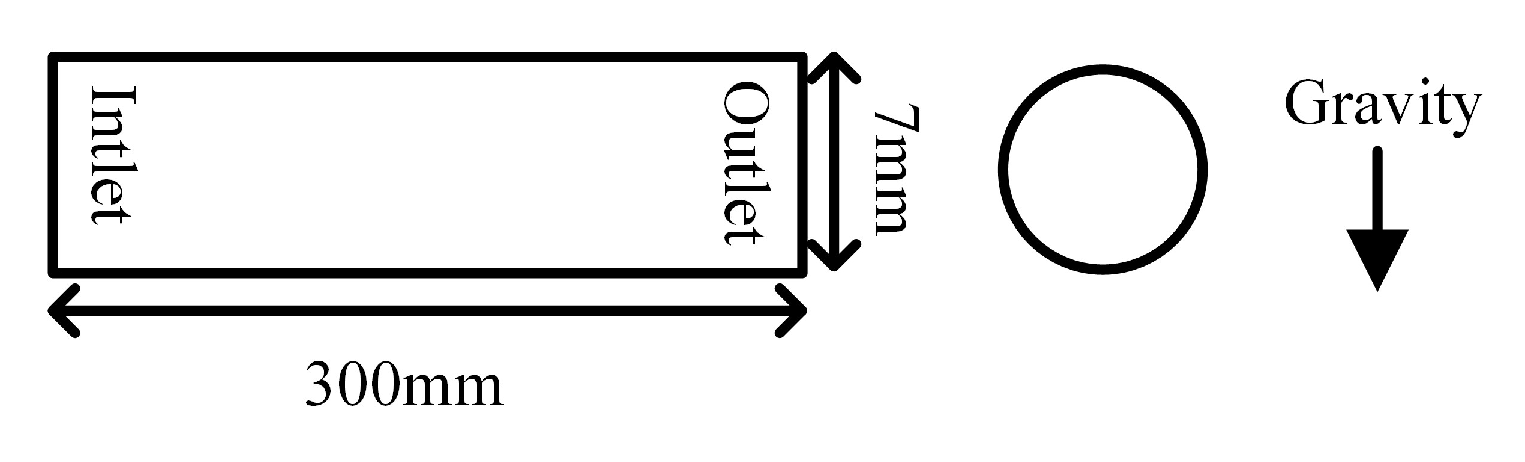
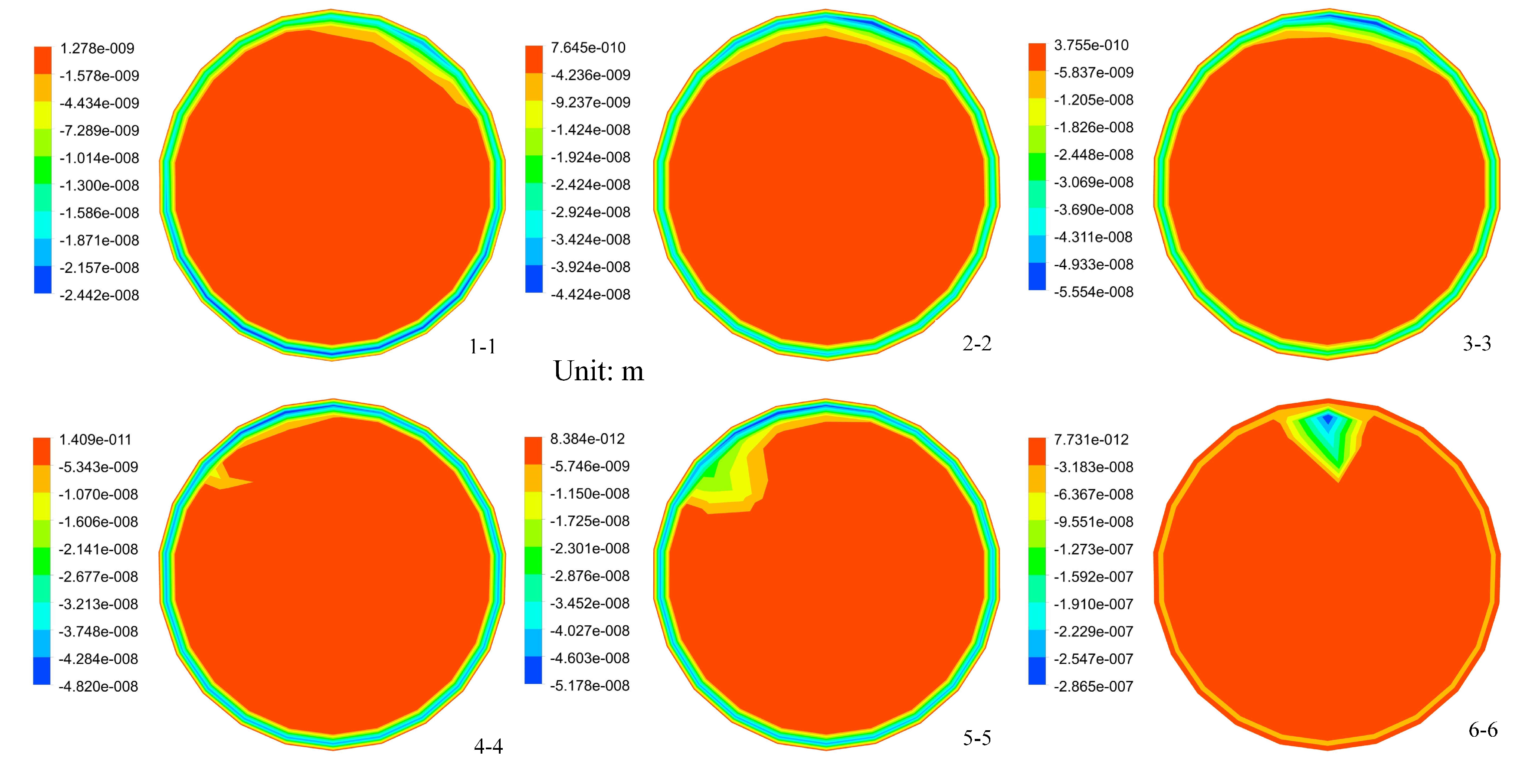
5. Model Verification

The first step in the model verification is to determine the bubble location. The experimental data from Reference [35] is used to calculate the value of the coefficient, $C$, which reflects the bubble location information. The subcooled fluid without the second phase gas flows into the heating pipeline after a free flow, and the experiment is observing the heating pipeline fluid flow. The simulation ignores the free flow, and the uniform subcooled liquid is set as the initial flow. The sketch of the experiment apparatus is shown in Figure 5. The flow rate G is 283.1 kg/m²s, the subcooled temperature is less than the saturation temperature of Pressure 1.23 bar 19.7 K.

Four levels of C are chosen to compare the corresponding void fraction with the experimental results, which are 0.6, 0.7, 0.8 and 0.9, as shown in Figure 6. Along the flow direction, the experimental void fraction increases from the inlet to the outlet. For the C = 0.6 and 0.8 cases, there are steep decreases of the void fraction around 75 mm away from the inlet, which are opposite to the experimental trend. For the C = 0.7 and 0.9 cases, the distributions of the void fraction along the tube length are similar to the experiment. Comparing with the C = 0.7 case, the C = 0.9 case provides a closer prediction to the experimental data, in which the relative error is smaller than 15%. The biggest gap between the C = 0.9 simulation and the experiment is in the near-inlet section. Since the simulation ignores the free flow section in front of the heating section in the experiment, the error can be accepted. As a result, C = 0.9 is adopted in the bubble diameter model.

The experiment conducted in Reference [4] is used for the model verification, as shown in Figure 7. The void fraction and the temperature along the tube length are calculated under the same operating condition using the proposed model and compared with the experiment. Figure 8 shows the calculated void fraction and temperature overlaid by the experimental results. It can be seen in Figure 8a that the calculated void fraction agrees with the experiment data well with relative errors no more than 20% in most cases. The biggest difference between the simulation and the experiment is at the position 1.5 m away from the inlet, where the liquid temperature has a higher value than the experiment, as shown in Figure 8b. The gas phase generates from axial distance about 0.6 m, and has a sharp increase at 1.1 m. The void fraction arrives at 40.74% at the outlet. Similar errors occur in the liquid temperature, as shown in Figure 8b. The biggest error is at the void fraction of 0.2 because the wall boiling heat transfer becomes non-equilibrium subcooled boiling when the void fraction is more than 0.2. It means the gas convection heat transfer cannot be ignored in the non-equilibrium subcooled boiling. The relative error of the wall temperature is smaller. The wall temperature reaches a peak of 543 K at 1.54 m, then falls to 541 K and keeps stable until the outlet. Comparing with the experimental data, the precision of the proposed model can be accepted in the flow boiling evaluation. Moreover, the bubble diameter model developed in this paper is appropriate for different operation conditions, in particular for different pressures.

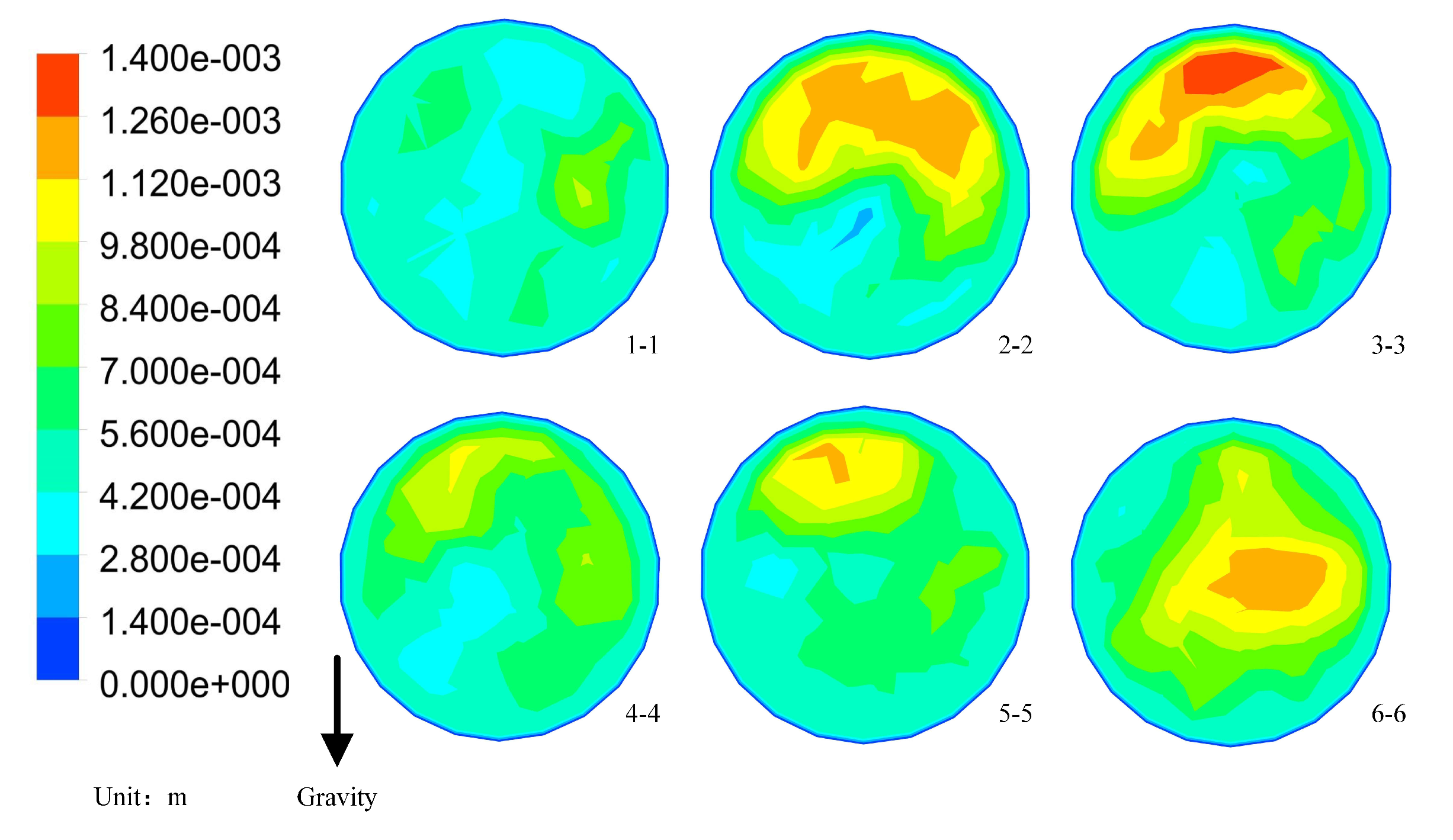
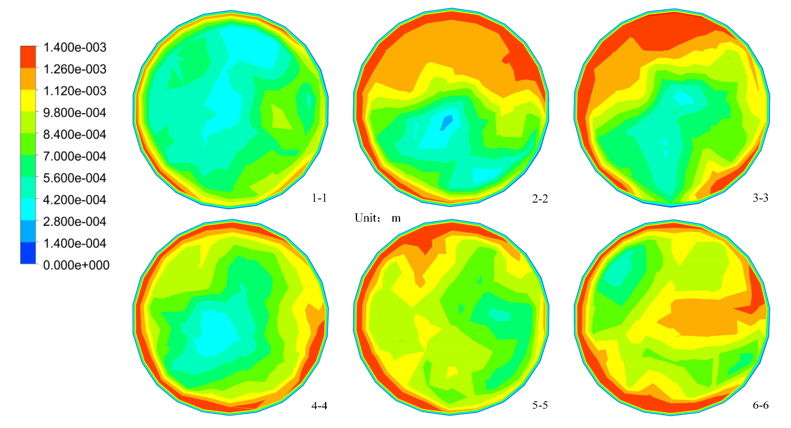
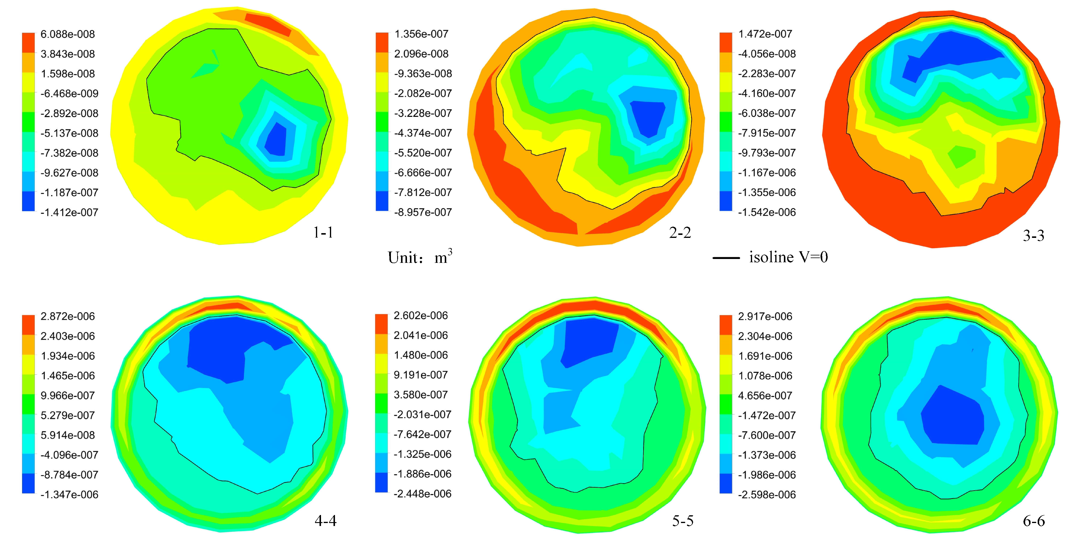
6. Case Study and Discussion

With the validated model, a case study is carried out to discuss the availability of the proposed model in different conditions. The simulations are conducted with a 300 mm long horizontal tube with inner diameter of 7 mm, which is long enough to produce bubbles and the gravity effect can be considered, as shown in Figure 9. The operation conditions are listed in

Table 1. Operation conditions.

Case	Operation Pressure (KPa)	Wall Temperature (K)	Inlet Velocity (m/s)	Inlet Temperature (K)
(a)	90	374	1	366
(b)	90	377	1	366
(c)	100	377	1	366

.

The calculated bubble size distribution along the tube is shown in Figure 10. For the horizontal tube studied, the flow in this specific case is affected by the gravity, which makes the gas phase concentrate in the upper part of the tube when the velocity is relatively low. Overall, the distribution of the bubble size is different from case to case. It is because different boundaries lead to different superheat, and the evaporation/condensation rate varies accordingly. The amount of the gas phase changes the flow type and the phase interaction force decides the velocity. Consequently, the bubble diameter components vary along with the flow development and result in totally different bubble size distributions. The maximum of bubble is approximately 1.4 mm in all three cases, and the differentiation is the distance that produces the large bubbles. In other words, the maximum size of bubbles that can be formed is 1.4 mm under such a pipe diameter and thermal conditions. From the comparison between Cases (a) and (b), it can be seen that a higher wall temperature tends to increase the bubble size except for the inlet area. The comparison between Cases (b) and (c) indicates the bubble size decreases with increasing operating pressure, especially in the middle section of the tube. The effect of pressure can also be regarded as the effect of the subcooled temperature because a higher operation pressure can bring a higher saturation temperature. Due to the constant physical parameters in these cases with, the Eotvos number $Eo=\frac{g\Delta \rho d_b^2}{\sigma }$ related to the diameter of the bubble is a diverse distribution with a maximum of 3.19 and minimum of about 0, and the Morton number $Mo=\frac{{\mu }^{4}g\Delta \rho }{{\rho }^2{\sigma }^3}$ is a constant, equal to 2.885 × 10⁻⁶. Thus, only some smaller shape deformations of the bubble might happen in these cases. The external forces mainly change the size of the bubbles.

Six sections along the tube length are chosen to show the bubble diameter distribution in the axial view in Case (b), as shown in Figure 11. In Section 1 and Section 6, the large bubble size concentrates at the center of the tube. In the four other sections, the big bubbles tend to generate in the upper half of the tube. A pattern of the bubble size distribution can be concluded that bubbles of large diameter move to the center of the tube when the flow is close to the outlet, which is affected by the exit ejection of the tube. If the constant value bubble diameter or approximately linear and temperature-dependent bubble diameter model applied in these cases, there will be a fixed value in entire flow field regardless of temperature and speed change or a series of rings bubble diameter distribution, which are all inconsistent with actual fact.

Bubble diameter distributions due to heat transfer are shown in Figure 12, those due to collision are shown in Figure 13, and those due to fluid impact are shown in Figure 14. In Figure 12, the maximum bubble diameter appears in the near-wall region where the liquid temperature is the highest. The flow boiling occurs in the subcooled condition, so the growth rate is less than zero according to the bubble diameter decrease. The upper part of the front half of the tube owns a greater heat transfer growth rate, as shown in Figure 12 (Section 2 and Section 3). The high heat transfer growth rate region varies along the tube and the area reduces as the flow approaches to the outlet because the temperature difference gets smaller. Ignoring the wall (the blue boundary), the bubble diameter distribution along the radial direction has local changes due to turbulence. Apart from that, the heat transfer results in an annular distribution of the bubble diameter in the subcooled boiling. The components due to heat transfer change from 0 mm to 1.4 mm, which is close to the maximum bubble diameter. In other words, the heat transfer contributes most to the bubble size in this case.

Figure 13 shows the distribution of the bubble diameter variation due to collision. $d_{collision}$ is positive in the main-flow region while it is negative in the near-wall region. That is to say, when the collision occurs in the main flow region, the possibility of coalescence is higher than that of breakup. In contrast, the collision in the near-wall region would result in more breakups than coalescences. The breakup contribution is in the range of 10⁻⁸ to 10⁻⁷ m while the coalescence contribution is 10⁻⁹ to 10⁻¹² m. Even if the integral is considered, those two terms are still not significant (10⁻⁵ to 10⁻⁴ m for breakup and 10⁻⁶ to 10⁻⁹ m for coalescence). In the front half tube, the influence of collision on the bubble size distribution is very slight even if the integral is considered. In the rear half, the proportion of the gas phase increases and the break up efficiency during the bubble collisions increases as well in the tube top. It is because the collision becomes more intensive as the gas phase increases to a certain extent, which has a higher efficiency of breaking up. The coalescence efficiency reduces due to the collisions frequency decrease of the full developed flow in the rear half. In short, the collision prompts the bubble diameter distribution to form two regions in the nuclear flow boiling, a ring high incidence area of bubble break up to decrease bubble diameter and a round high incidence area of bubble coalescence to increase bubble diameter.

Figure 14 is the distributions of the separating volume at different sections. A negative V region cannot separate the gas so that the separating volume region in Figure 14 is outside the isoline of V = 0 where the phase interaction force exceeds gas viscous force. At the inlet of the tube (Section 1), the separating volume region widely distributes around the wall. In this area, the separating volume contribution to the overall bubble diameter is around 1 mm, which is big enough to cover the heat transfer term. The orange area with around 1.1 mm in bubble size in Section 1 is the combination of the heat transfer term (1.07 mm) and the collision component (0.01 mm). As the flow develops along the tube length, the gas separating phenomenon becomes increasingly obvious in the first half of the tube. The maximum separating volume occurs at the bottom of the tube and then expands as a wide ring around the wall, as shown in Section 2 and Section 3. After that, the gas separating area continues to increase and the maximum region falls back to the top of the near-wall region. The maximum of separating volume component increases from 10⁻⁸ m to 10⁻⁶ m and maintain the size to the outlet, which means the speed difference gradually increases until stability. The separating volume changes also indicate that the flow is fully developed in the rear half of the tube. In Section 5, the heat transfer component of 1.4 mm, the collision component of −0.1 mm and the separating volume component of about −10 mm totally break the bubble in the near-wall region. The separating volume makes the overall bubble diameter decrease more obviously compared with the other two diameter components. In the flow, the heat transfer is the main contribution of the increment of the bubble diameter, but the overall diameter cannot increase infinitely because of the departure criterion. It can be described as a process that a growing bubble of a certain size of diameter bears the external force which reduces the bubble diameter and the process consists of growing and shrinking at the same time. The specific values of the increment and the decrement depend on the interaction between factors. The non-equilibrium force produces an annular break-up region surrounding that without break-up to decrease the bubble diameter. The break-up region slightly moves up due to the horizon flow and the gravity.

7. Conclusions

A new bubble diameter model is developed for the flow boiling simulation. The bubble diameter is divided into four components: the departure diameter, the diameter due to heat transfer, the diameter due to collision, and the diameter due to phase interaction force. Based on the proposed bubble diameter model, a flow boiling simulation scheme is established and carried out through C language and Fluent software. Main conclusions can be drawn:

(1)

The proposed overall diameter model can be regarded as a combination of the initial diameter and contributions from heat transfer, collision and phase interaction force. It is suitable for more operation conditions and can describe the void fraction and the temperature of the flow boiling accurately in different operating pressures and temperatures.

(2)

Comparing to linear correlations, the proposed model shows a more dispersed distribution of the bubble diameter inside the channel. Seen from the section distribution, the bubbles of large size spread over a wide asymmetric area instead of the evenly annular distribution of linear correlations.

(3)

Among the components of the overall bubble diameter, the variation due to heat transfer is considered as the dominant part controlling the bubble size. Meanwhile, the bubble diameter is also limited by the phase interaction force. The contribution from the collision is the smallest in the overall bubble diameter.

References

1. Filho, F.A.B.; Ribeiro, G.B.; Caldeira, A.D. Prediction of subcooled flow boiling characteristics using two-fluid Eulerian CFD model. Nuclear Eng. Des. 2016, 308, 30–37. [Google Scholar] [CrossRef]
2. Kenarsari-Anhari, A.; Leung, V.C.M.; Lampe, L. Numerical and experimental investigation on the effects of diameter and length on high mass flux subcooled flow boiling in horizontal microtubes. Int. J. Heat Mass Transf. 2016, 92, 824–837. [Google Scholar]
3. Gao, Y.; Shao, S.; Xu, H.; Zou, H.; Tang, M.; Tian, C. Numerical investigation on onset of significant void during water subcooled flow boiling. Appl. Therm. Eng. 2016, 105, 8–17. [Google Scholar] [CrossRef]
4. Bartolomei, G.G.; Chanturiya, V.M. Experimental study of true void fraction when boiling subcooled water in vertical tubes. Therm. Eng. 1967, 14, 123–128. [Google Scholar]
5. Saha, P.; Zuber, N. Point of net vapor generation and vapor void fraction in subcooled boiling. Analyst 1974, 112, 259–261. [Google Scholar]
6. Tu, J.Y.; Yeoh, G.H. On numerical modelling of low-pressure subcooled boiling flows. Int. J. Heat Mass Transf. 2002, 45, 1197–1209. [Google Scholar] [CrossRef]
7. Anglart, H.; Nylund, O. CFD application to prediction of void distribution in two-phase bubbly flows in rod bundles. Nuclear Eng. Des. 1996, 163, 81–98. [Google Scholar] [CrossRef]
8. Končar, B.; Kljenak, I.; Mavko, B. Modelling of local two-phase flow parameters in upward subcooled flow boiling at low pressure. Int. J. Heat Mass Transf. 2004, 47, 1499–1513. [Google Scholar] [CrossRef]
9. Yun, B.J.; Splawski, A.; Lo, S.; Song, C.H. Prediction of a subcooled boiling flow with advanced two-phase flow models. Nuclear Eng. Des. 2012, 253, 351–359. [Google Scholar] [CrossRef]
10. Lo, S.; Zhang, D. Modelling of break-up and coalescence in bubbly two-phase flows. J. Comput. Multiph. Flows 2009, 1, 23–38. [Google Scholar] [CrossRef]
11. Colombo, M.; Fairweather, M. Accuracy of Eulerian–Eulerian, two-fluid CFD boiling models of subcooled boiling flows. Int. J. Heat Mass Transf. 2016, 103, 28–44. [Google Scholar] [CrossRef]
12. Fritz, W. Berechnung des maximal volume von dampfblasen. Phys. Z. 1935, 36, 379–388. [Google Scholar]
13. Phan, H.T.; Caney, N.; Marty, P.; Colasson, S.; Gavillet, J. A model to predict the effect of contact angle on the bubble departure diameter during heterogeneous boiling. Int. Commun. Heat Mass Transf. 2010, 37, 964–969. [Google Scholar] [CrossRef]
14. Cho, Y.J.; Yum, S.B.; Lee, J.H.; Park, G.C. Development of bubble departure and lift-off diameter models in low heat flux and low flow velocity conditions. Int. J. Heat Mass Transf. 2011, 54, 3234–3244. [Google Scholar] [CrossRef]
15. Colombo, M.; Fairweather, M. Prediction of bubble departure in forced convection boiling: A mechanistic model. Int. J. Heat Mass Transf. 2015, 85, 135–146. [Google Scholar] [CrossRef]
16. Ruckenstein, E. On mass transfer in the continuous phase from spherical bubbles or drops. Chem. Eng. Sci. 1964, 19, 131–146. [Google Scholar] [CrossRef]
17. Cole, R. Bubble frequencies and departure volumes at subatmospheric pressures. AIChE J. 1967, 13, 779–783. [Google Scholar] [CrossRef]
18. Kocamustafaogullari, G.; Ishii, M. Interfacial area and nucleation site density in boiling systems. Int. J. Heat Mass Transf. 1983, 26, 1377–1387. [Google Scholar] [CrossRef]
19. Zuber, N. Hydrodynamic Aspects of Boiling Heat Transfer (Thesis); University of California: Los Angeles, CA, USA; Ramo-Wooldridge Corp.: Los Angeles, CA, USA, 1959. [Google Scholar]
20. Ünal, H.C. Maximum bubble diameter, maximum bubble-growth time and bubble-growth rate during the subcooled nucleate flow boiling of water up to 17.7 MN/m2. Int. J. Heat Mass Transf. 1976, 19, 643–649. [Google Scholar] [CrossRef]
21. Hoang, N.H.; Chu, I.C.; Euh, D.J.; Song, C.H. A mechanistic model for predicting the maximum diameter of vapor bubbles in a subcooled boiling flow. Int. J. Heat Mass Transf. 2016, 94, 174–179. [Google Scholar] [CrossRef]
22. Tolubinsky, V.I.; Kostanchuk, D.M. Vapour bubbles growth rate and heat transfer intensity at subcooled water boiling. In Proceedings of the International Heat Transfer Conference 4, Paris, France, 31 August–5 September 1970; Begel House Inc.: Danbury, CT, USA, 1970; Volume 23. [Google Scholar]
23. Nemitallah, M.A.; Habib, M.A.; Mansour, R.B.; Nakla, M.E. Numerical predictions of flow boiling characteristics: Current status, model setup and CFD modeling for different non-uniform heatingprofiles. Appl. Therm. Eng. 2015, 75, 451–460. [Google Scholar] [CrossRef]
24. Hibiki, T.; Ishii, M. One-group interfacial area transport of bubbly flows in vertical round tubes. Int. J. Heat Mass Transf. 2000, 43, 2711–2726. [Google Scholar] [CrossRef]
25. Shang, Z. A novel drag force coefficient model for gas–water two-phase flows under different flow patterns. Nuclear Eng. Des. 2015, 288, 208–219. [Google Scholar] [CrossRef]
26. Ranz, W.E.; Marshall, W.R. Evaporation from drops. Chem. Eng. Prog. 1952, 48, 141–146. [Google Scholar]
27. Del Valle, V.H.; Kenning, D.B.R. Subcooled flow boiling at high heat flux. Int. J. Heat Mass Transf. 1985, 28, 1907–1920. [Google Scholar] [CrossRef]
28. Cole, R. A photographic study of pool boiling in the region of the critical heat flux. AIChE J. 1960, 6, 533–538. [Google Scholar] [CrossRef]
29. Lemmert, M.; Chawla, J.M. Influence of flow velocity on surface boiling heat transfer coefficient. Heat Transf. Boil. 1977, 237, 247. [Google Scholar]
30. Behzadi, A.; Issa, R.I.; Rusche, H. Modelling of dispersed bubble and droplet flow at high phase fractions. Chem. Eng. Sci. 2004, 59, 759–770. [Google Scholar] [CrossRef]
31. Schiller, L.; Naumann, Z.Z. A drag coefficient correlation. Z. Ver. Deutsch. Ing. 1935, 77, 318–320. [Google Scholar]
32. Moraga, F.J.; Bonetto, F.J.; Lahey, R.T. Lateral forces on spheres in turbulent uniform shear flow. Int. J. Multiph. Flow 1999, 25, 1321–1372. [Google Scholar] [CrossRef]
33. Antal, S.P.; Lahey, R.T., Jr.; Flaherty, J.E. Analysis of phase distribution in fully developed laminar bubbly two-phase flow. Int. J. Multiph. Flow 1991, 17, 635–652. [Google Scholar] [CrossRef]
34. Burns, A.D.; Frank, T.; Hamill, I.; Shi, J.M. The favre averaged drag model for turbulent dispersion in Eulerian multi-phase flows. In Proceedings of the 5th International Conference on Multiphase Flow, ICMF, Yokohama, Japan, 30 May–6 June 2004. [Google Scholar]
35. Zeitoun, O.; Shoukri, M. Axial void fraction profile in low pressure subcooled flow boiling. Int. J. Heat Mass Transf. 1997, 40, 869–879. [Google Scholar] [CrossRef]
Figure 1. Presentation of the bubble flow in the wall flow boiling.
Energies 11 01297 g001
Figure 2. Presentations of bubble collision and break up.
Energies 11 01297 g002
Figure 3. Calculation frame of the overall bubble diameter.
Energies 11 01297 g003
Figure 4. Schematic of the bubble behavior and the heat transfer manner in the near-wall region.
Energies 11 01297 g004
Figure 5. Presentation of Zeitoun’s experiment [35].
Energies 11 01297 g005
Figure 6. Experimental and simulation void fractions.
Energies 11 01297 g006
Figure 7. Presentation of Bartolomei’s experiment [4].
Energies 11 01297 g007
Figure 8. Comparison of (a) the void fraction and (b) the temperature between the proposed model and Bartolomei’s experiment.
Energies 11 01297 g008aEnergies 11 01297 g008b
Figure 9. Presentation of the simulation case.
Energies 11 01297 g009
Figure 10. Bubble size distribution along the tube.
Energies 11 01297 g010
Figure 11. Bubble diameter distributions in Section 1, Section 2, Section 3, Section 4, Section 5 and Section 6.
Energies 11 01297 g011
Figure 12. Distributions of d d + d h e a t in Section 1, Section 2, Section 3, Section 4, Section 5 and Section 6.
Energies 11 01297 g012
Figure 13. Distributions of 2 d c o l l i s i o n / n in Section 1, Section 2, Section 3, Section 4, Section 5 and Section 6.
Energies 11 01297 g013
Figure 14. Distributions of separating volume in Section 1, Section 2, Section 3, Section 4, Section 5 and Section 6.
Energies 11 01297 g014