Computational Fluid Dynamic Modelling and Optimisation of Wastewater Treatment Plant Bioreactor Mixer ^†

Abstract

This study aims to determine the optimal configuration (position and operation duration) for wall mounted mechanical mixers based on the comparison of three-dimensional computational fluid dynamics (CFD) modelling results and physical data collected from the treatment plant. A three dimensional model of anoxic zone in 1, 2 and 3 of Northern Wastewater Treatment Plant (NWWTP) located at Cairns Regional Council, Cairns, Queensland, Australia was developed and validated. The model was used to simulate the flow pattern of the WWTP and the simulation results are in good agreement with the physical data varying between 0% to 15% in key locations. The anoxic zones were subject to velocities less than the desired 0.3 m per second however results for mixed liquor suspended solids (MLSS) concentration indicate that good mixing is being achieved. Results for suspended solids concentrations suggest that the anoxic zones are towards the upper limits recommended by literature for specific power dissipation. The duration for operation of mechanical mixers was investigated and identified that the duration could be reduced from 900 s down to 150 s. Alternative mixer positioning was also investigated and identified positioning which would increase the average flow velocity with decreased duration (150 s). The study identified that Council may achieve savings of $28,500 per year through optimisation of the mechanical mixers and would be expected to extend the operational life of the mixers.

1. Introduction

A Waste Water Treatment Plants (WWTP) is an industrial facility where a combination of mechanical, physical, chemical and biological processes is used to achieve pollutant removal from the incoming wastewater [1]. WWTP are used to treat and process raw sewage prior to discharging into water ways. These facilities are commonly operated and resourced by local governments and are critical infrastructure assets that need to be fully operational, all year round in Australia.

Wastewater treatment can be one of the largest components of overall energy use by local governments and there are significant opportunities for reducing the required electrical input into WWTP [2]. The personal equivalent (PE) for Northern WWTP in 2016 was 80,368. The data was taken from Cairns council planning study of NWWTP completed in 2016 and for example, a typical energy breakdown for a 20ML NWWTP is as follows [3]:

• 42% activated sludge aeration;
• 20% influent pumping;
• 10% effluent filters;
• 6% thickening/dewatering centrifuges;
• 5% activated sludge mixing;
• 17% other (screens, returns activated sludge (RAS)/waste activated sludge (WAS) pumping & other)

As Council is financially supported by ratepayers, the increased cost in operating WWTPs will ultimately be borne by ratepayers either in the form of a rate increase or at the expense of reduced funds for capital works projects. The focus of this study is the NWWTP; one of the plants operated by Cairns Regional Council Water & Waste (CRCWW). NWWTP had a monthly average electricity cost of $57,000 in 2016; $54,000 in 2015 and $52,000 in 2014. The electricity cost of NWWTP represents 27% of the total cost of the top 15 CRCWW facilities for power consumption. 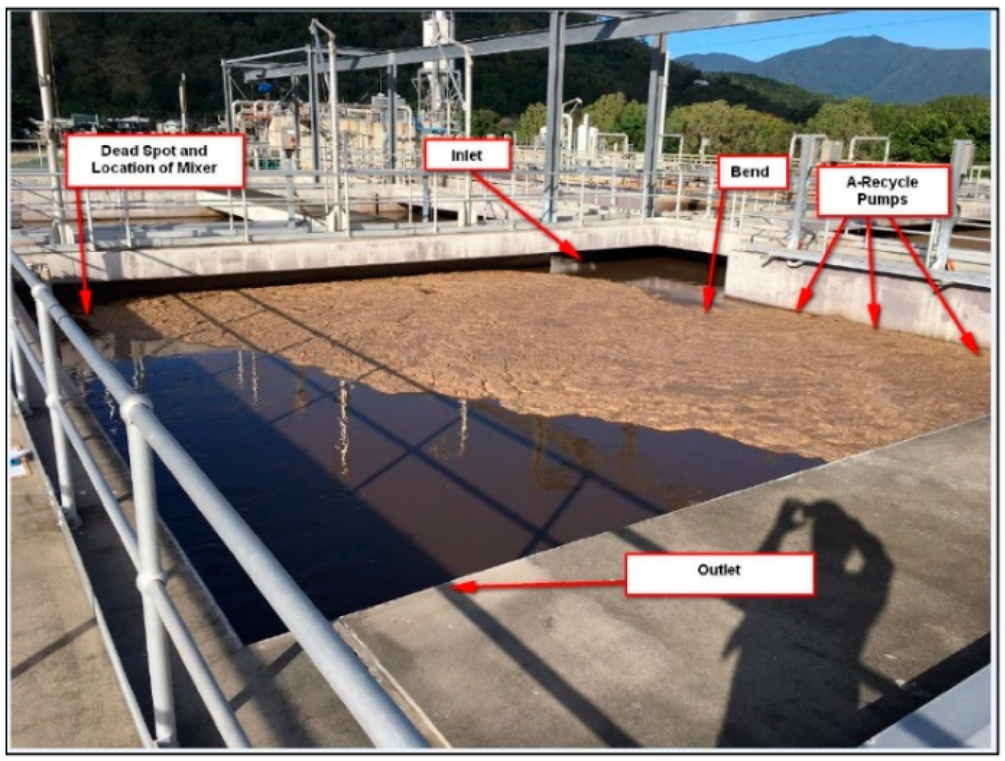The top 15 CRCWW facilities for power consumption in 2016 had a monthly average electricity cost of $210,000 whereas year to date monthly electricity cost for the same 15 facilities in 2017 averages $230,000 (January to August) [4]. The bioreactor consists of three 25 kW variable speed drive (VSD) A-recycle pumps and eight 7.6 kW submersible mixers.

With the Cairns region experiencing an 18% increase in population over the last decade [5] and as the price of electricity is anticipated to increase in the coming years, an investigation into the optimal configuration of submersible mixers was undertaken to explore a decrease of operation time for the mixers, or the number of mixers required for the bioreactor. It is revealed that a review of the current submersible mixer configuration and its operation will result in a decrease in the electricity cost to operate the facility, potentially providing financial savings to the Council. This benefit could be compounded as the Council operates several other treatment facility of similar configuration.

A common type of treatment method is the activated sludge process. Raw sewage is treated in the bioreactor by replicating biological reactions similar to that which occurs naturally. The raw sewage flows through the bioreactor with each zone providing different biological reactions to assist in the removal of pollutants such as nitrogen and phosphorus compounds [6]. The NWWTP bioreactor investigated is a compartmentalized activated sludge process and the main treatment component of the NWWTP is the bioreactor which is shown in Figure 1. The bioreactor is a multi-compartment box type structure where biological organisms break down and remove the contaminants within the sewage. The Cairns Regional Council’s NWWTP is a 20-mega-litre (ML) activated sludge compartmentalized bioreactor consists of the following zones.

• Four anoxic zones
• Four aerobic zones
• Three anaerobic zones

The NWWTP bioreactor consists of several pumps and mixers which promote the fluid flow as shown in

Table 1. Mixer configuration per zone in bioreactor.

Zone		Motor Size	Motor Type
Anoxic 1	A-Recycle Pump 1	25 kW	Variable Speed Drive
Anoxic 2	A-Recycle Pump 2	25 kW	Variable Speed Drive
Anoxic 3	A-Recycle Pump 3	25 kW	Variable Speed Drive
Pre Anoxic	Mixer	7.6 kW	Direct Online
Anaerobic 1	Mixer	7.6 kW	Direct Online
Anaerobic 2	Mixer	7.6 kW	Direct Online
Anaerobic 3	Mixer	7.6 kW	Direct Online
Anoxic 1	Mixer	7.6 kW	Direct Online
Anoxic 2	Mixer	7.6 kW	Direct Online
Anoxic 3	Mixer	7.6 kW	Direct Online
Anoxic 4	Mixer	7.6 kW	Direct Online

. The current configuration of the mixers allows for either continuous or intermittent operation. Currently the mixers are configured to run for 15 min before switching off for 15 min. This is repeated over a 24-h period, seven days a week, all year round. This configuration was based on the original design of the plant when handed over to Council. Based on the typically power break down for a 20 ML WWTP, the activated sludge mixing at NWWTP cost $35,000 per year.

The NWWTP consists of a primary, secondary and tertiary treatment process. The majority of pollutants that can settle or float are removed by screens; this is the primary treatment process. The secondary treatment process occurs in the plants bioreactor. The treatment process simulates biological reactions similar to that which occur naturally in an aquatic environment [6]. The tertiary process involves further treatment such as membrane filtration before the effluent is discharged into a river catchment. 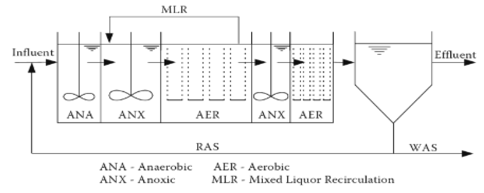Figure 2 represents the treatment process at Northern WWTP were the bioreactor contains an anaerobic zone, anoxic zone and aerobic zone.

The NWWTP bioreactor consists of the following zones; Anaerobic, Anoxic and Aerobic. Each zone is designed to provide different environmental conditions to allow for the microorganisms within that zone the best opportunity to treat the influent similar to that shown in Figure 2. The concentration of biodegradable carbon and nitrogen is measured in Biological Oxygen Demand (BOD) and is a measure of dissolved oxygen required by microorganisms to convert the organic matter. Therefore, excessive carbon and nitrogen in waterways will require additional dissolved oxygen to break down and therefore potentially deprive fish and other aquatic organisms of oxygen and/or promoting the growth of algae [8]. The Queensland Department of Environment and Heritage Protection stipulate the BOD limits on the issued licenses for discharging wastewater in Queensland waterways, thus the limits can vary depending on the location and size of the treatment facility. However, a best practice environment management limit of 2 mg/L for BOD is recommended [9].

Changes to the operational parameters may influence the quality of the discharged processed sewage and this may have an impact on the ability to comply with the environmental licensing conditions of the facility. The flow regime and mixing phenomena within an activated sludge bioreactor can be assessed experimentally through tracer techniques. However, the size of full scale plants generally renders this unfeasible [10]. As such, Council is hesitant to modifying operations without undertaking a performance review.

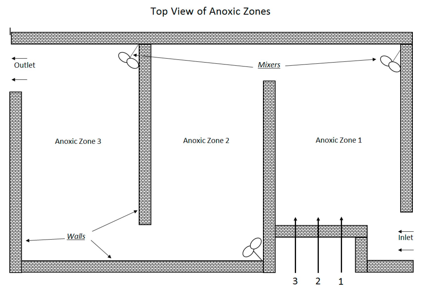
Computational Fluid Dynamic (CFD) is a tool to facilitate this review. To analyse the performance of the anoxic zone 1, 2 and 3, CFD modelling was undertaken in this study to determine the fluid flow pattern. A 3D CFD model of anoxic zone 1, 2 and 3 was developed to simulate the expected fluid flow. The CFD model results were validated by the physical data collected from the NWWTP that is operated by Council and allowed for a review of the fluid flow through the anoxic zones, therefore assessing the performance of the current configuration of submersible mixers. The desired outcome of the study is to predict the optimal configuration for wall mounted mixers based on the comparison of CFD modelling results to physical data collected from the treatment plant.

2. Waste Water Treatment Design

The major influence on the design of the WWTP is the desired pollutant removal rate, which can be determined mathematically. This however is based on assumed hydrodynamics of the bioreactor [11]. Current wastewater treatment design methods make assumptions of the mixing conditions and it is therefore difficult to predict how bioreactor design (i.e., position of inlet, baffles, or membrane structures) affect hydrodynamics, hence overall performance [12].

Traditionally, prior to modern technology, Engineers would have to undertake a repetitive and time-consuming process of designing, modelling and validating bioreactor designs to ensure that the fluid flow behaviour performed as expected. In addition, the mixer configuration and influence of this configuration could not be accurately modelled on a prototype designs. However, as demonstrated by Brannock [11], the modelling of hydrodynamics effects of bioreactor configuration in large-scale situations can be undertaken thanks to the development of sophisticated CFD modelling and increased computational power which has contributed to the successful spread of CFD within both academia and industry [12].

To overcome the assumption of hydrodynamic performance of a bioreactor and to maintain MLSS concentration throughout the bioreactor, mixers could be installed in various positions to promote fluid flow [13]. CFD modelling can provided a reasonably accurate method for prediction of how the bioreactor features and mixing energy usage affects the hydrodynamics [14].

3. Minimum Bioreactor Velocities

As micro-organisms are used to react with nitrogen and phosphorus within the bioreactor zones, poor fluid flow may result in settlement and therefore decrease performance in the removal of biodegradable matter. To overcome the issue of settlement, submersible mixers may be used if the velocity within the zone is considered too low. As noted by Brannock [11] the minimum velocities required to overcome settlement has been extensively researched by academics and the wastewater treatment industry. Brannock [11] stated that a minimum velocity of 0.1 m per second (m/s) was previously thought to be adequate. However, it has been revised and suggested that 0.3 m/s is required as a minimum velocity to avoid settlement of micro-organisms. Previous simulation and modelling results by Elshaw et al. [15] indicated that anoxic zone 1 of the NWWTP was maintaining adequate suspension of total solids with no mechanical mixers in two of the four test locations, this was due to the influence of the inlet and outlet on flow velocity.

4. Specific Power Dissipation

The specific power dissipation is useful to determine if a zone is over powered by mechanical mixers thus contributing to waste of energy. The literature suggests [10] a target or range for the specific power dissipation and that the typical power requirements of 8 to 13 W/m³ for mechanical mixers within an anoxic zone. Furthermore, this is supported by the recommendation from the Water Environment Federation which recommends that the power requirements for mixing as 1 W/m³ [10].

To evaluate the performance of the submersible mixers, the specific power dissipation can be calculated from the equation below that uses the dynamic viscosity of the fluid and the solid concentration [16].

$$P_s=0.0582{\mu }^{0.3}{C}_{XS}^{0.298}$$

(1)

where μ is the dynamic viscosity, Pa∙s and C_XS is the solid concentration in kg/m³.

The concentration of solids in the raw sewage would influence the fluid properties with respect to fluid density. For simplicity, it is assumed that the primary treatment process removes all solids and floating matter from the raw sewage. Therefore, the properties of raw sewage will assume to exhibit the same properties of water.

5. A-Recycle Pump Configuration

The anoxic zone 1 has three 25 kW VSD pumps which are controlled either automatically depending on the inflow into the plant, or manually depending on the needs of the facility.

6. Submersible Mixer Configuration

Each anoxic zone contains one 7.6 kW submersible mechanical mixers. The mixers are generally located 1 m above the floor and directed toward the opposite corner of the zone at 20 degrees above horizontal. Mixers are configured for intermittent operation for 15 min on and 15 min off. The succeeding zone mixers will alternative on and off times.

7. Research Methodology

7.1. Experimental

The major influence on the design of the WWTP is the desired pollutant removal rate, which can be determined mathematically. This however is based on assumed hydrodynamics of the bioreactor. As said, the NWWTP is fully operational in the Cairns Regional Council. Therefore, only physical data were extracted from the plant for the validation of the simulation results. Data acquisition method has already been installed in the NWWTP and is described below.

7.2. Collection of Physical Data

Preliminary data was collected from the treatment plant and was used to validate the CFD model. Velocity readings were collected using a Marsh McBirney Flo-mate velocity probe, all of which were taken at approximately 0.5 m off the wall and at 1 m depth increments at 12 locations. It is noted that limited access was available to the outlets due to the configuration of guardrails. Cairns Regional Council supplied the probe. The probe would display readings to two significant figures and therefore the error from the probe is assumed to be ± 0.005 m/s. The probe was calibrated prior to use and therefore the results obtain can be considered accurate.

7.3. CFD Modelling and Simulation

In this study, CFD modelling is the prime consideration for the prediction of flow behaviour inside the bioreactor. To develop the initial model in ANSYS Fluent, the geometry of the structure must first be defined. The geometry for the anoxic zone model was developed using Design Modeller and then the geometry was imported into ANSYS Fluent for meshing. As previously stated, the CFD modelling and analysis was undertaken for anoxic zone 1, 2 & 3 in the NWWTP bioreactor that described in Figure 1 and Figure 3 shows the geometry with mesh and define functions.

The three-dimensional model was constructed with the default meshing options and then each of the function of the model were named accordingly, for example, walls, inlet, A-recycle pump, mixers and outlet. The inlets are denoted in yellow, mixers are denoted orange and the outlets are denoted in green as shown in Figure 3. The inlet to anoxic zone 1 and 3 is via a 3.5 m × 2.72 m opening located at the top of the zone and via a 0.8 m × 3.5 m opening located at the bottom of the zone. The outlet to anoxic zone 1 and 3 is via a 3.5 m × 2.72 m opening located at the bottom of the zone and via a 3.5 m × 0.8 m opening at the top of the zone. The A-Recycle pumps are 0.8 m in diameter located 0.75 m of the bottom water level and the mixers are 0.58 m in diameter located 1 m above the bottom water level and are positioned facing the opposite corner and angled 20° above horizontal. The three-dimensional model mesh independence was based on previous work completed by Elshaw et al. [15].

The standard K − ω turbulence model was used in this study for solving turbulent flow. It is based on transport equations for the turbulence kinetic energy (K) and the specific rate of dissipation (ω). The standard K − ω transport equation was developed by Wilcox [17] which was formulated to better compute low-Reynolds number effects, compressibility and shear flow spreading [18]. The standard K − ω transport equation is suitable for complex boundary layer flows under adverse pressure gradient and separation [19]. Similar CFD modelling studies which investigated the reproduction of model results compared to physical results, noted that the K − ω turbulent model more closely compared with the physical results. Whereas the K − ε turbulent model underestimated the model results [12,15].

7.4. Boundary Conditions

The boundary conditions of each zone were defined according to the published literature [20]. The different sections of the geometry perimeter were named in regard to their desired function; Walls, Inlet, Outlet & Mixers as shown in Figure 4 to ensure that they had been correctly interpreted by Fluent. Walls were defined as Walls and the inlet and A-Recycle pump velocity of 0.166 m/s and 0.860 m/s were entered for the respective inlets while the outlet was selected at a pressure-outlet of 0 Pa. The liquid temperature was considered as 29 °C and the density of fluid was assumed of 996 kg/m³.

8. Results and Discussion

Previous studies by Elshaw [15] identified that while less complex, 2D modelling is not able to correctly illustrate the hydrodynamic profile of the bioreactor, therefore a 3D CFD modelling was completed.

8.1. 3D CFD Results

The results from the 3D model can illustrate regions within the anoxic zone that are likely to experience high or low velocities and can also provide a better understanding of how the geometry of the structure can influence the flow behaviour. Previous studies identified that as 2D modelling does not factor the depth of the zone and the vertical distance between zone features it results in a vastly different flow profile compared to 3D modelling. Figure 5 illustrates the flow path of anoxic zone 1 from the A-Recycle pump and inlet as seen from the top view of the zone [15]. For these reasons, this study has focused solely on 3D modelling.

Xie et al. [21] confirmed that 3D modelling can reveal more details with respect to the flow behaviour and can provide designers with a better understanding of how structure geometry influences fluid flow within a zone.

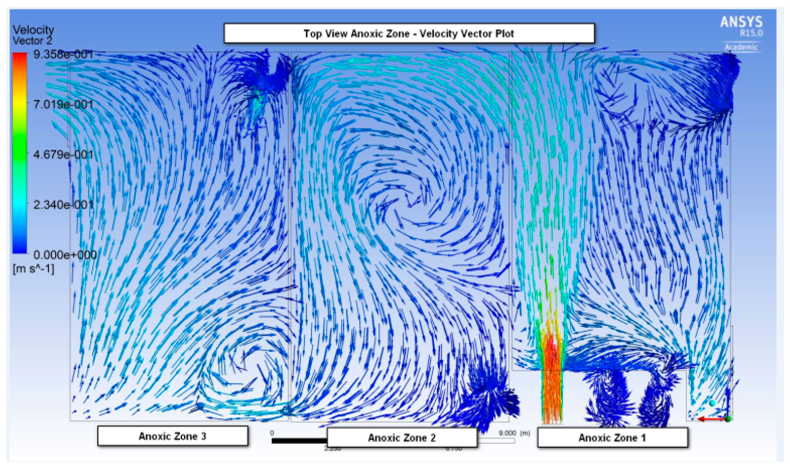
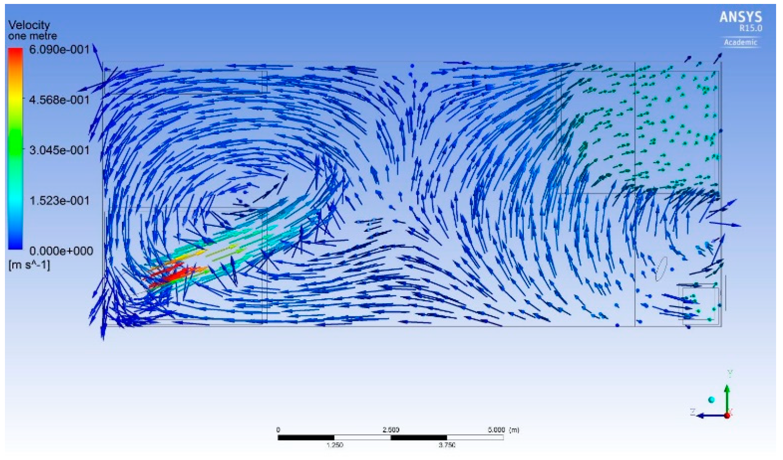
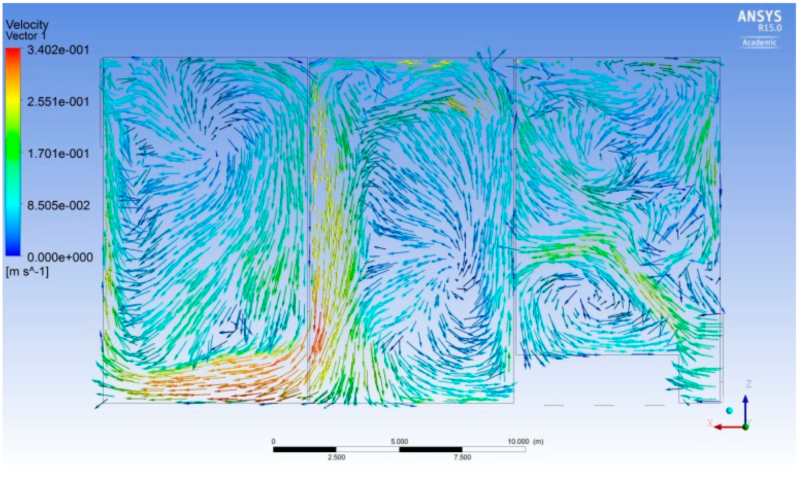
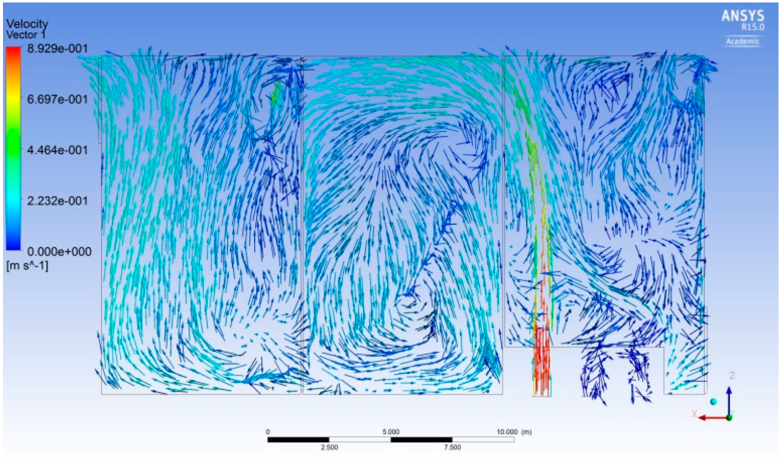
The velocity vector plots illustrate the flow path and the corresponding velocities through the three anoxic zones and the influence of the inlets, A-Recycle pump and submersible mixers. As stated by Brannock [11] the minimum recommended velocity to prevent settlement of micro-organisms is 0.3 m/s. The results from the simulation incorporating the submersible mixers indicate that majority of the velocities across the three zones are below the recommended 0.3 m/s. Regions which demonstrated velocities above 0.3 m/s are within the path of the A-Recycle pump and mixers. Furthermore, the larger inlet into each anoxic zone resulted in a flow velocity greater than 0.2 m/s. The position of the larger inlet into each zone alternates between the bottom water level and the top water level. The velocity vector plot for 1 m depth and 5 m depths illustrates this flow pattern as seen in Figure 6 and Figure 7.

Further illustrated from Figure 6 and Figure 7, are the influence of the openings into each zone and the creation of vortices. The vortices are a result of regions of low velocity, shearing with the higher velocity flows entering from the zone’s inlet [22].

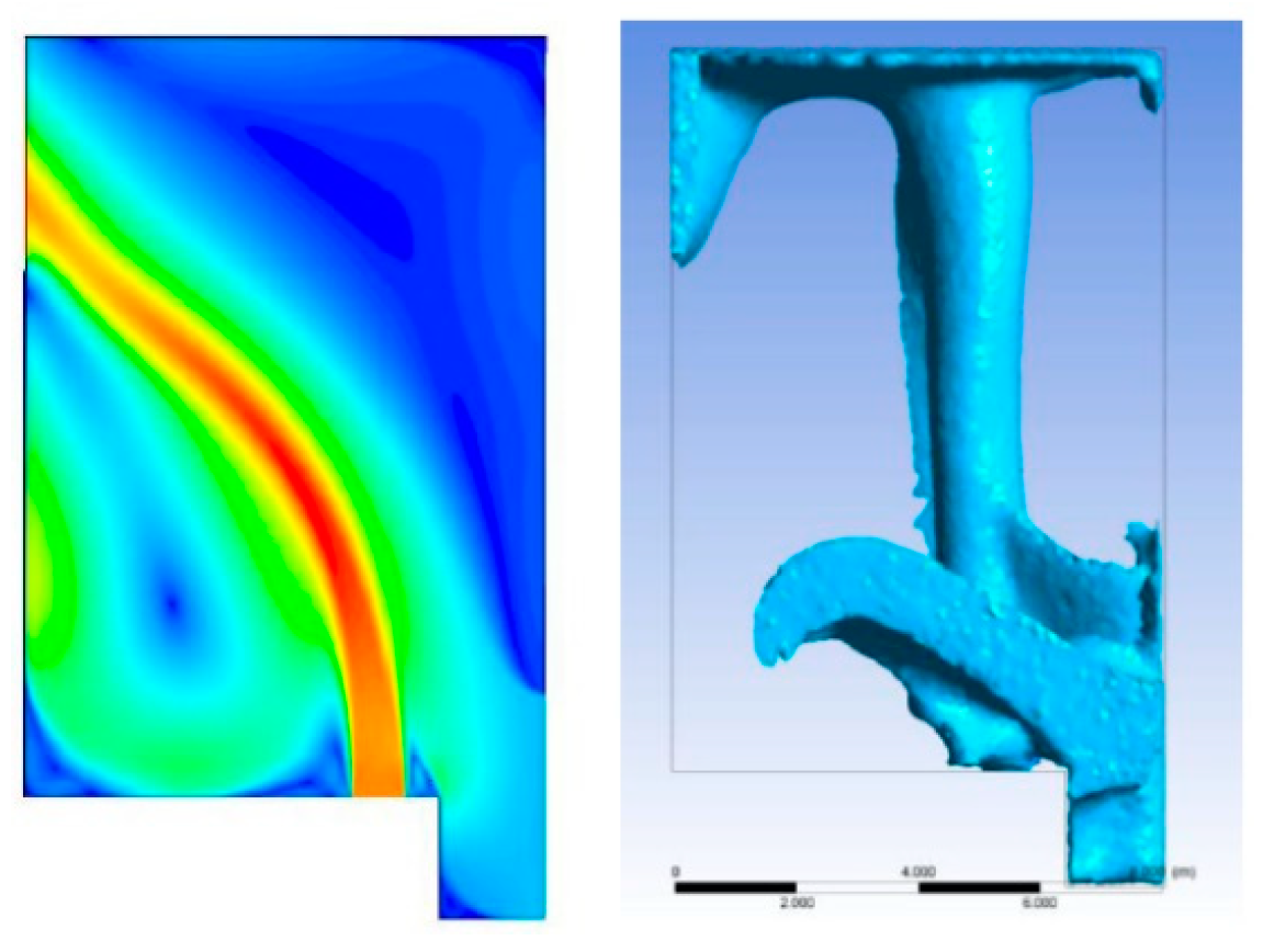
The velocity vector plot in the ZY plane in anoxic zone 3 illustrates the direction of flow from the submersible mixer and the influence of the prominent flow path. The region below the mixer experiences low velocity of approximately 0.1 m/s and therefore settlement of micro-organisms may occur in this region as seen in Figure 8.

The velocity vectors also indicate that short circuiting may be occurring across all three anoxic zones. Short circuiting is where the flow moves directly from the inlet of a zone to the outlet with minimal to no contact with the fluid in other regions of the same zone. This may impact on the biological reactions and the denitrifying process. Short circuiting can be further illustrated from the streamline path plots.

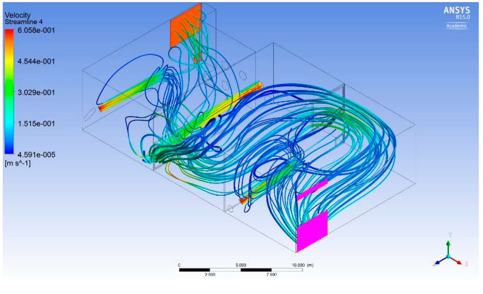
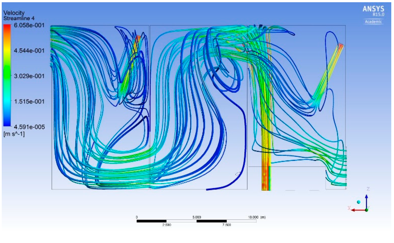
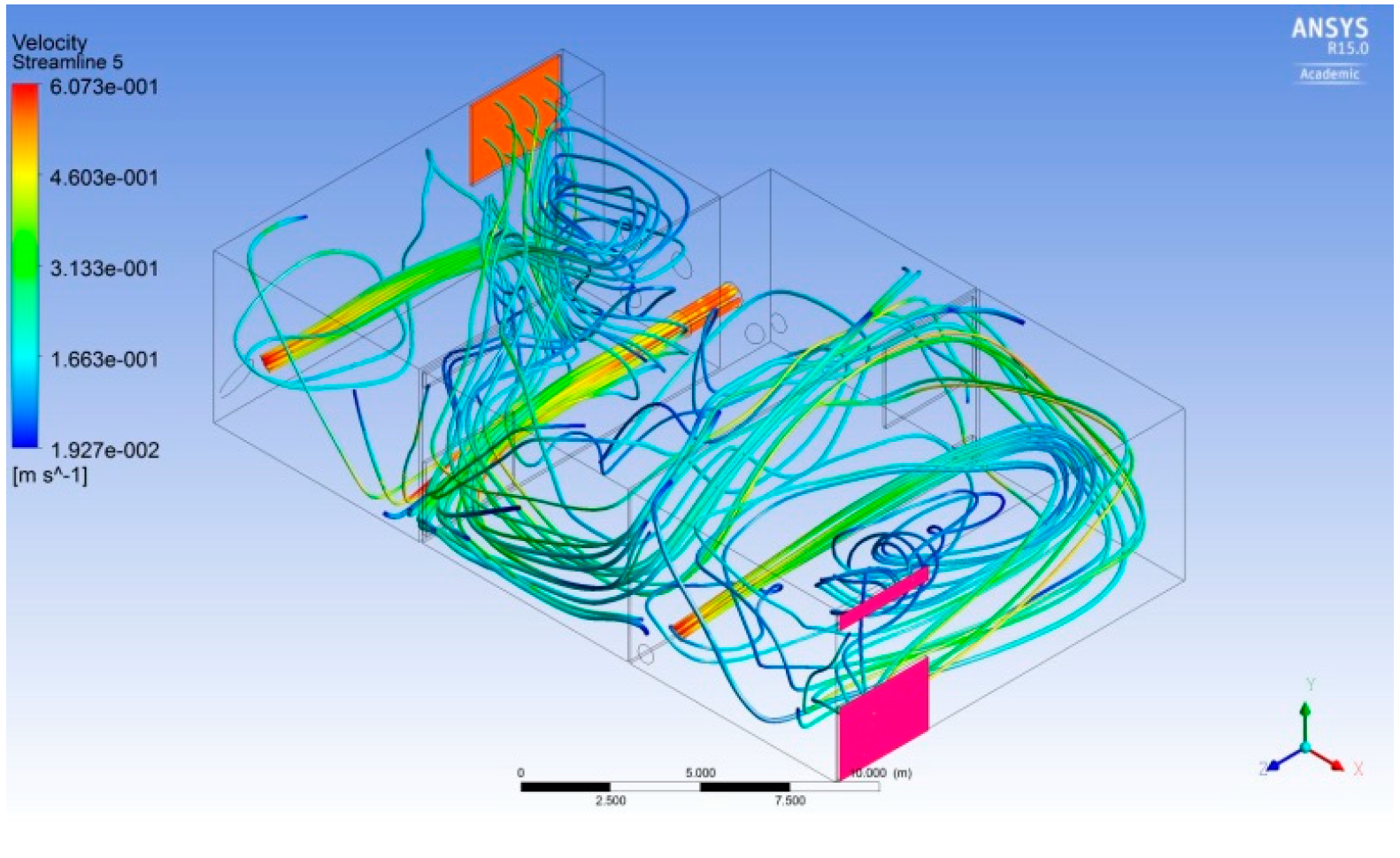
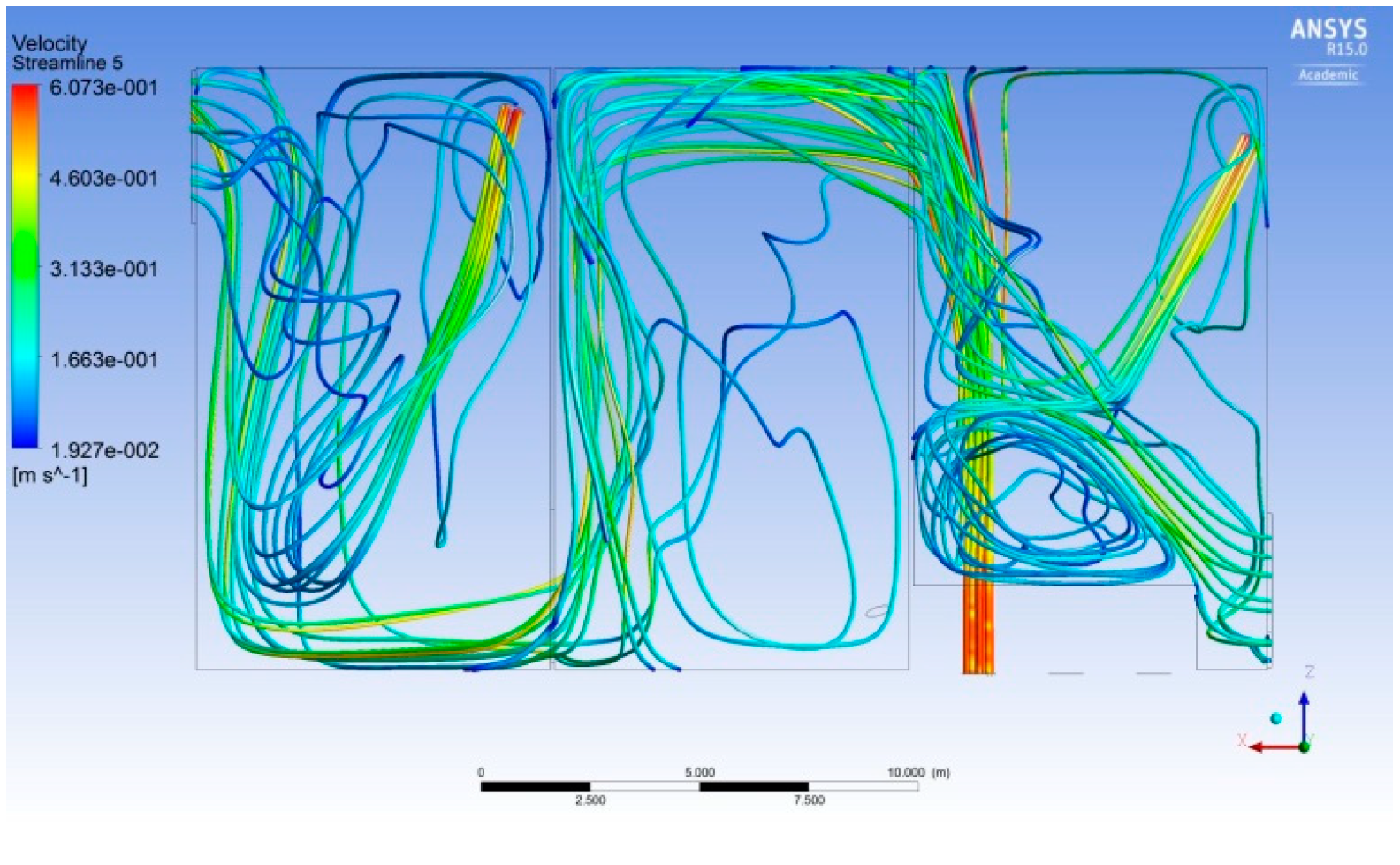
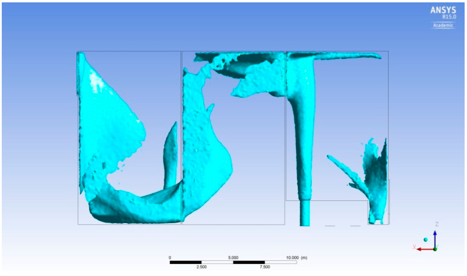
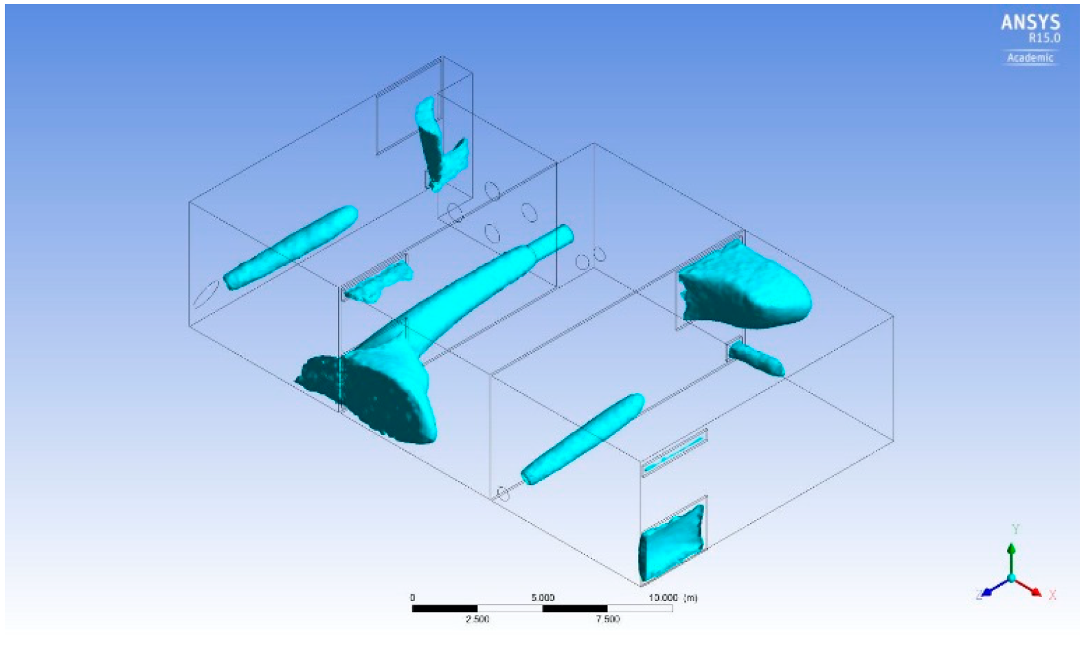
The streamline path plot further highlights regions within the three anoxic zones which experience a velocity less than recommended, while including the performance of the submersible mixers. The streamline path plot shows that across the three anoxic zones, the location of the submersible mixers is outside of the prominent flow path. It is within these regions where the velocity is less than 0.3 m/s as seen in Figure 9 and Figure 10.

The mixers are not able to influence the velocity adjacent to their location, due to the direction in which they face. Alternative mixer locations may assist to achieve a more dissipated flow path across the three anoxic zones.

Figure 9 and Figure 10 show mixer 1 and 3 operating. The flow from the mixers continues until it reaches the prominent flow path from the A-Recycle pump and anoxic zone inlet. The prominent flow path limits the distance in which the flow from the mixers would have propagated.

From the 3D CFD simulation results of the current submersible mixer configuration, the submersible mixers do not appear to assist with mixing within each anoxic zone. The flow from the mixers propagates outwards towards the prominent flow path of the bioreactor, where it is curved toward the outlet of the zone. This results in majority of anoxic zone 1, 2 and 3 experience velocities below 0.3 m/s as shown in the three velocity vector plots (Figure 6, Figure 7 and Figure 8).

8.2. Validation of CFD Modelling Results

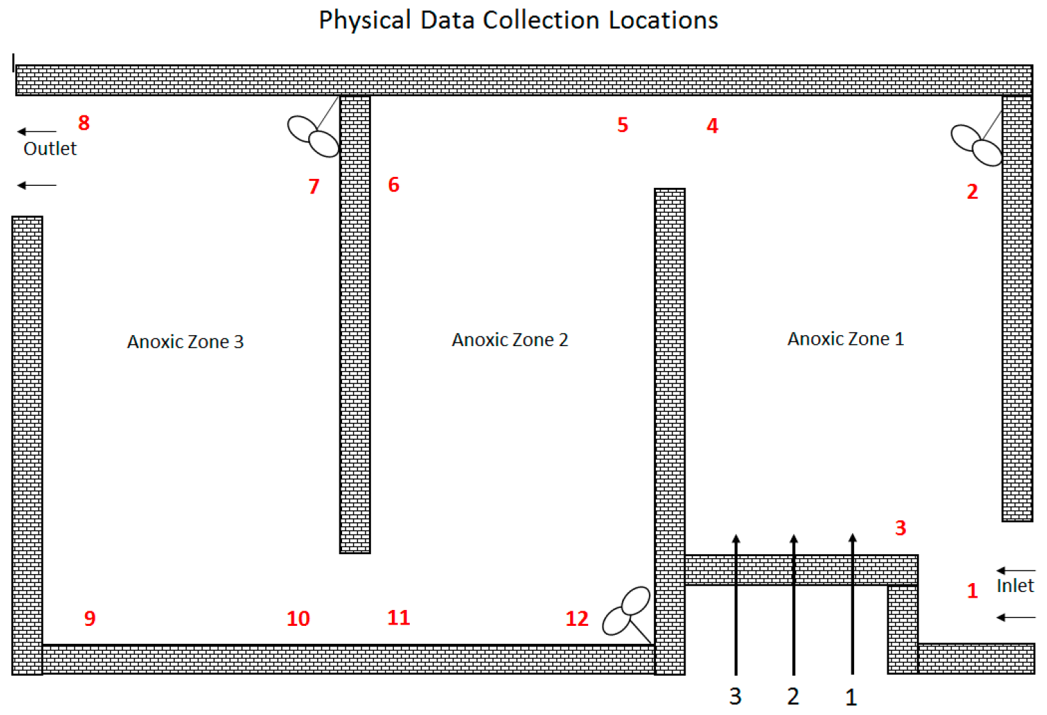
Physical data on the velocities and suspended solids were collected from Northern WWTP. Velocity data were collected using a Marsh McBirney Flow meter. Velocity readings were taken at 12 locations across the three anoxic zones at one meter depth increments down to three meters. The length of the velocity cable limited the depth which readings could be recorded. Due to the varying nature of plant inflows, the velocity at each location was observed for a period with the minimum and maximum readings recorded and averaged.

Table 2. Velocity results and comparison between CFD model and physical samples.

Location 1
Depth	Physical Velocity	Model Velocity	Variance
1 m	0.125 m/s	0.11 m/s	12%
2 m	0.13 m/s	0.14 m/s	7%
3 m	0.06 m/s	0.06 m/s	0%
Location 2
3 m	0.045 m/s	0.05 m/s	10%
Location 3
1 m	0.085 m/s	0.075 m/s	12%
2 m	0.125 m/s	0.115 m/s	8%
3 m	0.125 m/s	0.11 m/s	12%
Location 4
1 m	0.06 m/s	0.07 m/s	14%
Location 5
1 m	0.05 m/s	0.045 m/s	10%
3 m	0.105 m/s	0.11 m/s	5%
Location 6
1 m	0.03 m/s	0.035 m/s	14%
3 m	0.03 m/s	0.035 m/s	14%
Location 8
1 m	0.045 m/s	0.05 m/s	10%
3 m	0.113 m/s	0.115 m/s	2%
Location 9
1 m	0.06 m/s	0.07 m/s	14%
Location 10
1 m	0.145 m/s	0.145 m/s	0%
2 m	0.165 m/s	0.155 m/s	5%
3 m	0.106 m/s	0.125 m/s	15%
Location 11
1 m	0.1 m/s	0.105 m/s	5%
2 m	0.11 m/s	0.115 m/s	4%

details the physical average velocity recorded and the variance between the CFD model and physical data. Only data that varied by 15% has been reported on.

Figure 11 illustrates the 12 location of physical data collected.

The above tables illustrates that the CFD model of anoxic zone 1, 2 and 3, is in good agreement with the physical data.

8.3. Suspended Solids

Physical data on the suspended solids was collected in May 2017 at Northern WWTP. Suspended solids data was collected using a Royce Suspended Solids meter and collected at one m increments below the surface and the results were recorded.

During the collection of physical data of suspended solids, mixer 2 is switched off when mixer 1 and mixer 3 operate. The mixers operate for 15 min on before switching off for 15 min and during this off period the adjacent zone mixer switches on. It is noted that zone 4 and mixer 4 was not included in the simulation in this study.

The concentration of suspended solids can be utilised to determine the specific power dissipation and thus if a zone is wasting energy from mechanical mixers. The suggested range from literature for specific power dissipation is 8 W/m³ to 13 W/m³. The concentration of suspended solids ranged from 4.16 g/L to 4.75 g/L. The results of the suspended solids per sample location in kg/m³ and depth is presented in

Table 3. Suspend Solids Concentration per sample location and depth (kg/m³).

Location	Depth (metres)
	1 m	2 m	3 m	4 m	5 m
Location 1	4.63	4.67	4.72	4.75	4.45
Location 2	4.52	4.3	4.6	4.57	4.57
Location 3	4.31	4.52	4.57	4.3	4.44
Location 4	4.53	4.55	4.57	4.55	4.67
Location 5	4.58	4.54	4.57	4.61	4.63
Location 6	4.44	4.37	4.52	4.37	4.48
Location 7	4.46	4.32	4.16	4.45	4.62
Location 8	4.32	4.16	4.24	4.36	4.46
Location 9	4.31	4.26	4.66	4.46	4.52
Location 10	4.52	4.55	4.52	4.7	4.65
Location 11	4.37	4.38	4.52	4.44	4.61
Location 12	4.41	4.43	4.17	4.27	4.39

.

The temperature of the sewage was recorded as 29 °C during the collection of physical data. The equation developed by Grady and Lim was used to determine the specific power dissipation. For the equation shown in equation 1, the temperature of the sewage at 29 °C corresponded to a dynamic viscosity of 8.15 × 10⁻⁴ Pa∙s and the suspended solid concentration in kg/m³ was determined to be 1.96 kg/m³ [15].

Utilising Grady and Lim specific power dissipation equation, the following results in

Table 4. Specific Power Dissipation per sample location and depth (W/m³).

Location	Depth (metres)
	1 m	2 m	3 m	4 m	5 m
Location 1	13.5	13.6	13.6	13.6	13.4
Location 2	13.4	13.2	13.5	13.5	13.5
Location 3	13.2	13.4	13.5	13.2	13.4
Location 4	13.4	13.4	13.4	13.4	13.5
Location 5	13.4	13.4	13.4	13.5	13.5
Location 6	13.3	13.2	13.4	13.2	13.3
Location 7	13.3	13.2	13.1	13.3	13.5
Location 8	13.2	13.1	13.1	13.2	13.3
Location 9	13.2	13.1	13.5	13.3	13.4
Location 10	13.4	13.4	13.5	13.5	13.5
Location 11	13.2	13.3	13.4	13.3	13.5
Location 12	13.3	13.3	13.1	13.2	13.3

are obtained for the specific power dissipation per sample location and depth based on the values shown in Table 3.

The specific power dissipation results are above the upper limit of 13 W/m³ recommended by literature. Good mixing is considered to be achieved when there is less than a 10% difference in the suspended solids concentration throughout the zone. The only zone which recorded a difference greater that 10% is location 7, which had a difference of 11%. This abnormality may be attributed to the positioning of the suspended solids probe or the make of sewage at the time of physical sample collection.

Elshaw et al. [15] completed testing of the suspended solid concentrations and specific power dissipation in anoxic zone 1 at Northern WWTP with the mechanical mixers switched off [15]. The results from this test identified that the zone was toward the lower limit of specific power dissipation with a range of 8.2 W/m³ to 8.9 W/m³.

The operational duration of the mechanical mixers can be reduced based on the results for specific power dissipation. Elshaw et al. [15] specific power dissipation results in 2016 with mechanical mixers turned off in anoxic zone 1 indicated specific power requirements towards the lower end of the range recommended by the literature at 8 W/m³. Specific power dissipation results including the mixers in anoxic zone 1, 2 and 3 indicate that the specific power is above the upper end as recommended in the literature at 13 W/m³. Therefore a reduction in the operating duration of the mechanical mixers would result in a specific power dissipation requirement within the range as recommended in the literature. The current specific power dissipation results for anoxic zone 1, 2 and 3, indicate that some energy in being wasted as results are above the recommend 13 W/m³.

8.4. Predict Optimal Design

The research also investigated the potential minimum duration which the mixers would be required to operate for and the location which could enhance their application. The current configuration of mixers alternates on and off for 900 s (15 min). A number of simulations were performed for different durations and the flow profile observed.

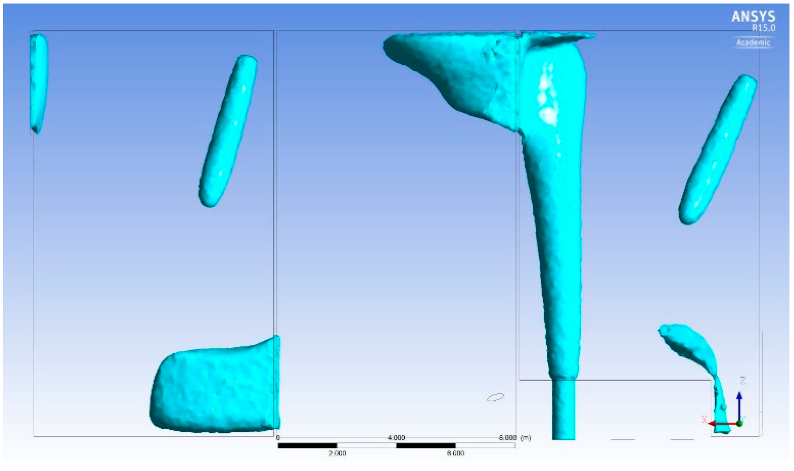
A simulation was performed which had the mixers in zone 1 and 3 operator for 150 s (2.5 min). The streamline path plots illustrated that the flow from the mixers was more prominent than that of the 900 s simulation as shown in Figure 12 and Figure 13.

The increased duration which the mixers operate reduces the effectives of their application. Therefore shorter durations of operation appear to be more affective in achieving the required velocity and promoting mixing.

The increase in velocity magnitude can also be observed in comparing the velocity vector plots for the alternative mixing duration with that of the current configuration as shown in Figure 14 and Figure 15. The flow profile is similar, however the magnitude has increased.

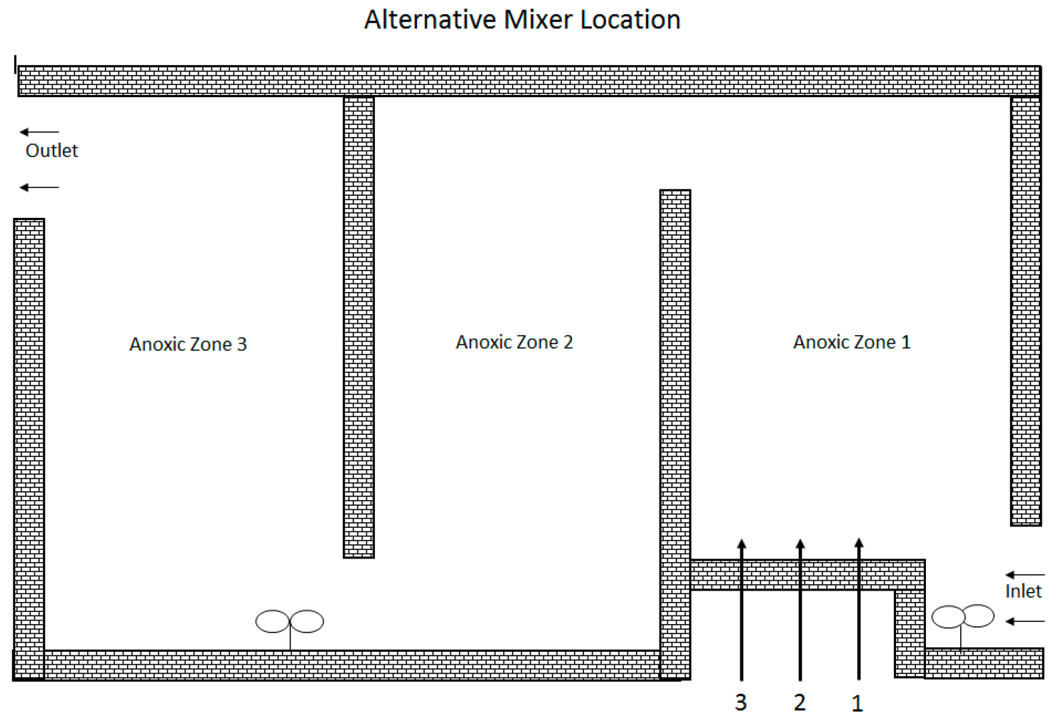
The positioning of the mixers was also investigated. Their current position is illustrated in Figure 11. The alternative position of the mixers was located at the inlet to zone 1 and 3 as shown in Figure 16. The mixers were positioned between the two inlets into each zone to maximise the existing flow path.

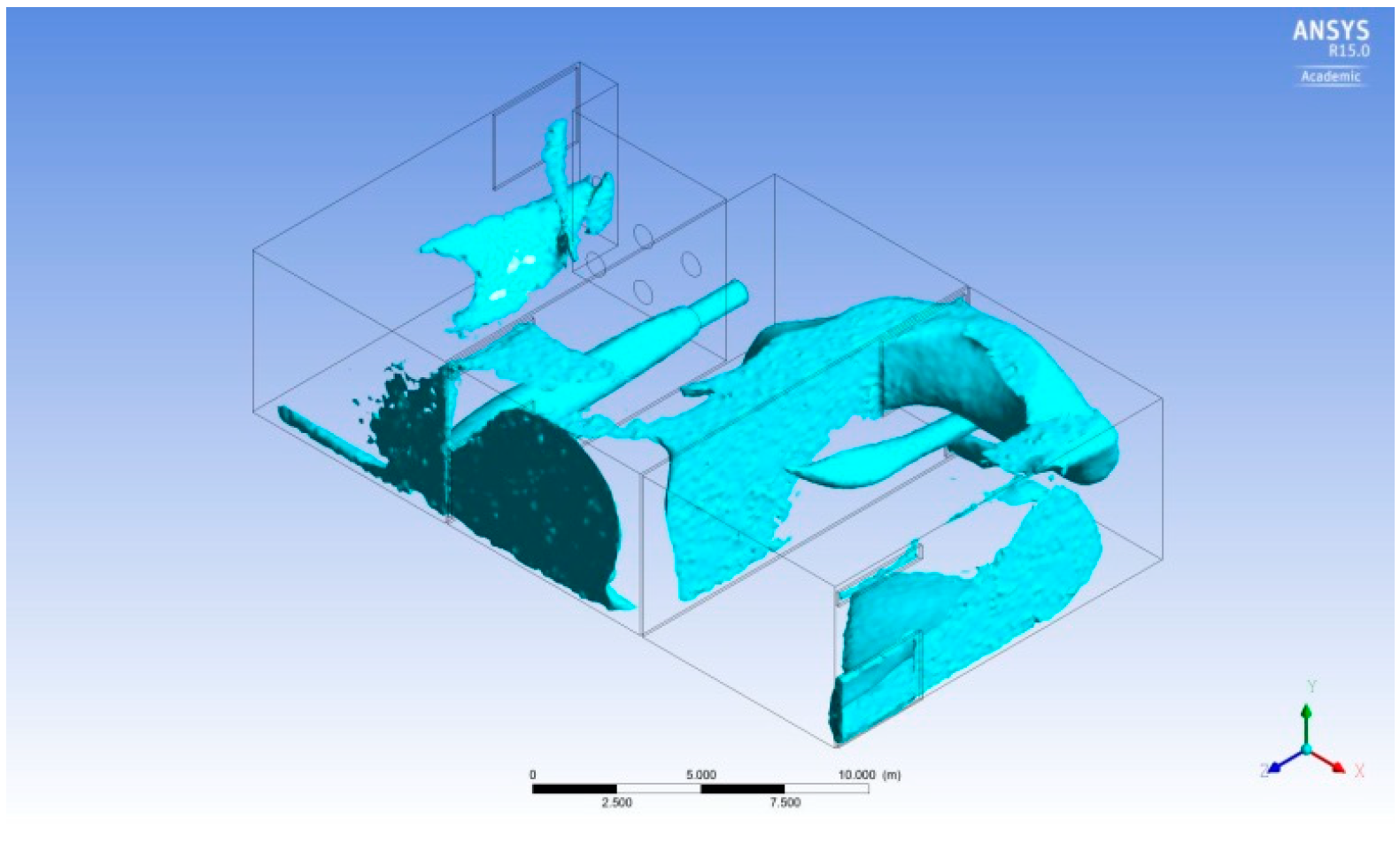
The simulation of the alternative position for mixers resulted in streamline paths from the mixers which propagated for the full length of each zone. As the flow from the mixers was not impeded by the bioreactor flow or A-Recycle pump, the simulation illustrated an overall increase is velocity through zones 1, 2 and 3. The increase in velocity can be observed between the two surface plots for velocities 0.2 m/s and greater for the alternative simulation and the current configuration as shown in Figure 17, Figure 18, Figure 19 and Figure 20.

The purpose of this simulation was to review and confirm if the 15 min operation of mixers is sufficient to achieve the required velocities and to review the flow profile. The results from the 15 min simulation in Figure 10 was compared against the 2.5 min simulation in Figure 13. It was noted from the physical data collected that the flow velocities observed were less than that recommended. Based on the simulation results from the 2.5 min simulation, the flow velocity within all the zones marginally increases and the flow from the mixers propagates further. The shorter duration of operation which shows an increase in flow velocity would assist to keep solids suspended and therefore the operation of the mixers could be reduced. The simulation only modelled the flow velocity while the mixers in zone 1 and 3 where operational. Further research could investigate the period of time for the flow to reduce following different operating durations (15 min, 10 min and 5 min) and also model the suspension of solids after similar operating durations. The 2.5 min simulation indicates that the duration of the mixers could be reduced, pending further investigation as stated. This would result in power savings as a result of reducing the duration of operation for the mixers.

9. Conclusions

The current configuration and position of the mixers resulted in specific power dissipation values on the upper limit (13 W/m³) of the recommendation by literature and therefore potentially wasting energy by over mixing the anoxic zones 1, 2 and 3. This is further demonstrated by previous investigation completed by Elshaw et al. [15] on the suspended solids concentration in Anoxic Zone 1 without mixing. The suspended solids concentration ranged from 8.2 kg/m³ to 8.9 kg/m³. Specific power dissipation results above 13 W/m³ indicates that energy is being wasted and therefore the duration which the mixers operate can be reduced. A reduction in the operation duration would lower the specific power dissipation results.

The average monthly electricity cost of the Northern WWTP in 2016 was $57,000 of which $2850 per month can be attributed towards mechanical mixing. By reducing the duration for which the mixers operates down from 900 s to 150 s, the monthly electricity costs for mechanical mixers could be reduced to $475 per month. This could potentially save Council $28,500 per year in electricity costs and would be expected to extend the operational life of the mixers.

The streamline path plots demonstrate that with a shorter duration of operation, the flow from the mixers propagate further in the zone compared to the current configuration which has the mixers operating for 900 s on and off.

The positioning of the mixers has also been investigated using the validated CFD model. By positioning the mixers at the inlet into zone 1 and 3 as illustrated in Figure 16, the flow from the mixers not being restricted by the flow within the bioreactor, resulted in an increase in average flow velocity. While anoxic zones 1, 2 and 3 still experience velocities less than the recommended 0.3 m/s for suspension of solids, the increase in flow velocity would be expected to improve the suspension of solids.

The validated CFD model of anoxic zones 1, 2 and 3 was able to demonstrate improvements to the anoxic zone by optimising the mechanical mixers. The Council is considering investigating with physical trials to explore possible reduction of the operation duration with the suggested alternative positions for mechanical mixers.

Further Research

The CFD models developed only performed simulations using A-Recycle pump 3. It would be expected that if simulations were performed using A-Recycle pump 2 or 1, a different flow profile would occur. This may alter the velocities experienced in anoxic zone 1 or potential that of zone 2 and 3.

Further simulation and investigation could look into the influence on flow velocities with only mixer 2 in anoxic zone 2 operating and investigate the impact in zone 3.

The Northern WWTP has a total of 4 anoxic zones. The fourth zone was excluded from this research to check the accuracy and validation of the simulation results. Simulation will be performed considering all 4 anoxic zones.

The study and its findings provide motivation/incentive for undertaking a similar approach to evaluate operational efficiency of Wastewater Treatment Plant.