An LM-BP Neural Network Approach to Estimate Monthly-Mean Daily Global Solar Radiation Using MODIS Atmospheric Products

Abstract

Solar energy is one of the most widely used renewable energy sources in the world and its development and utilization are being integrated into people’s lives. Therefore, accurate solar radiation data are of great significance for site-selection of photovoltaic (PV) power generation, design of solar furnaces and energy-efficient buildings. Practically, it is challenging to get accurate solar radiation data because of scarce and uneven distribution of ground-based observation sites throughout the country. Many artificial neural network (ANN) estimation models are therefore developed to estimate solar radiation, but the existing ANN models are mostly based on conventional meteorological data; clouds, aerosols, and water vapor are rarely considered because of a lack of instrumental observations at the conventional meteorological stations. Based on clouds, aerosols, and precipitable water-vapor data from Moderate Resolution Imaging Spectroradiometer (MODIS), along with conventional meteorological data, back-propagation (BP) neural network method was developed in this work with Levenberg-Marquardt (LM) algorithm (referred to as LM-BP) to simulate monthly-mean daily global solar radiation (M-GSR). Comparisons were carried out among three M-GSR estimates, including the one presented in this study, the multiple linear regression (MLR) model, and remotely-sensed radiation products by Cloud and the Earth’s radiation energy system (CERES). The validation results indicate that the accuracy of the ANN model is better than that of the MLR model and CERES radiation products, with a root mean squared error (RMSE) of 1.34 MJ·m⁻² (ANN), 2.46 MJ·m⁻² (MLR), 2.11 MJ·m⁻² (CERES), respectively. Finally, according to the established ANN-based method, the M-GSR of 36 conventional meteorological stations for 12 months was estimated in 2012 in the study area. Solar radiation data based on the LM-BP method of this study can provide some reference for the utilization of solar and heat energy.

1. Introduction

Due to the boom in population, urbanization, and industrialization, the energy demand has increased enormously, which causes rapid depletion of fossil fuel resources and pollution of the environment [1]. Solar energy is a cleaner and more renewable energy resource, and its development and utilization can greatly alleviate the negative environmental effects caused by the harmful substances released by the combustion of fossil fuels, such as air pollution, acid rain, the greenhouse effect, ecological balance, destruction and so on. Solar radiation is also the main energy source and the basic driving force on Earth, providing necessary energy for the water cycle, atmospheric motions, and biological activities [2]. Meanwhile, it is one of the necessary input parameters in the crop evapotranspiration model, ecosystem carbon and nitrogen cycle, hydrology, and climate-change models [3]. Therefore, making full use of solar energy resources has a significant impact on the strategy of sustainable development [4]. However, worldwide solar radiation observation sites are sparse and distributed unevenly. Lack of solar radiation data limits research works in relevant fields; thus, it is important to perform the simulation of solar radiation.

Many efforts have been made to simulate solar radiation in different geographical and climatic regions of the Earth. Some traditional simulation models such as Angstrom [5], Hargreaves-Samani [6], Meteorological Radiation Model (MRM V 6.1) [7], Bristow and Campbell [8], Akinoglu and Ecevit [9], Louche et al. [10] and the radiative transfer model [11] have been used; but these models have many limitations. First, these models rely on specific input parameters; the Angstrom model and MRM V 6.1 rely on the sunshine duration [7,12], and the Hargreaves-Samani model and Bristow and Campbell model depend on minimum and the maximum temperatures [6,13]. Second, the simulation process of these models is more complex. For example, the radiative transfer models need to calculate the transmittance function, such as Rayleigh scattering transmittance function, solar diffuse radiative transmittance function, aerosol transmittance function [14], which are difficult to get accurately, particularly for non-professionals. Therefore, the traditional model cannot be used effectively. In the past ten years, many scholars [15,16,17,18,19,20] have begun to use ANN models to simulate solar radiation. These research can be divided into several categories, including: (1) Comparing the simulation accuracy of ANNs with different input parameters. Rao et al. [21] used different combinations of daily minimum temperature (T_min), daily maximum temperature (T_max), the difference of daily maximum and minimum temperature (DT), sunshine duration (S₀), theoretical sunshine duration (S) and extraterrestrial radiation (H₀) to train an ANN; six ANN models were developed to estimate mean daily global solar radiation. The results that the showed a combination of DT and H₀ gave the best prediction of the Relative Root Mean Square Error (RRMSE), being as little as 3.96%; (2) Comparing neural network models with other models. Teket et al. [22] compared 91 models for simulating solar radiation; these models can be summarized as linear models, nonlinear models, mixed models, and neural network models. The percentage errors were 3.62%, 2.50% to 6.93%, 0.14 to 6.93%, and 0.30%, respectively; (3) comparing the neural network models with different algorithms. For example, based on the daily air temperature, air pressure, relative humidity, vapor pressure, and sunshine duration, Wang et al. [23] established the multilayer perceptron (MLP), generalized regression neural network (GRNN), and radial basis neural network (RBNN) solar radiation estimation models in different climate zones in China. The results indicated that the MLP and RBNN models are generally more accurate than the GRNN, with the RMSE values of 2–3.29 MJ·m⁻²·day⁻¹ for GRNN, 1.94–3.27 MJ·m⁻²·day⁻¹ for MLP, and 1.96–3.25 MJ·m⁻²·day⁻¹ for RBNN models. Moreover, many previous studies have shown that the simulation of solar radiation based on neural network present relatively high accuracy [24,25,26,27,28,29,30].

However, the existing ANN models for estimating solar radiation were mostly based on conventional meteorological data; the impact of clouds, aerosols, water vapor, and other factors were rarely considered because of a lack of instrumental observations at the conventional meteorological stations, as aerosols, clouds, and water vapor have a great impact on solar radiation. Fortunately, remote sensing (RS) techniques provide us with continuous signals from space and fill the gap of conventional meteorological stations data. Meanwhile, RS-based retrieval algorithms provide an alternative method to simulate solar radiation, such as the radiation transfer models, but its physical mechanism is too complex to be mastered for non-professionals. Moreover, current RS products of radiation contain coarse spatial resolutions (1° or more) [31].

To address these issues, the main objective of this study is to develop a simple and efficient method of solar radiation simulation, providing some reference data for areas with limited observations. Under the support of aerosol optical thickness (AOT), cloud fraction (CF), cloud optical thickness (COT), precipitable water vapor (PWV) from MODIS and conventional meteorological data, including air temperatures (T), sunshine duration (S₀), air pressure (P), vapor pressure (Pw), and relative humidity (RH), an LM-BP neural network model was established to estimate M-GSR in Shaanxi Province and its surrounding areas. Its performance was evaluated against the MLR and remotely-sensed radiation products by CERES. Further, according to the established LM-BP neural network model, the M-GSR of 36 conventional meteorological stations was estimated in the study area.

The remainder of this paper consists of four sections. The materials and methodology are described in Section 2. The results and discussion are provided in Section 3, and the conclusion is presented in Section 4.

2. Materials and Methodology

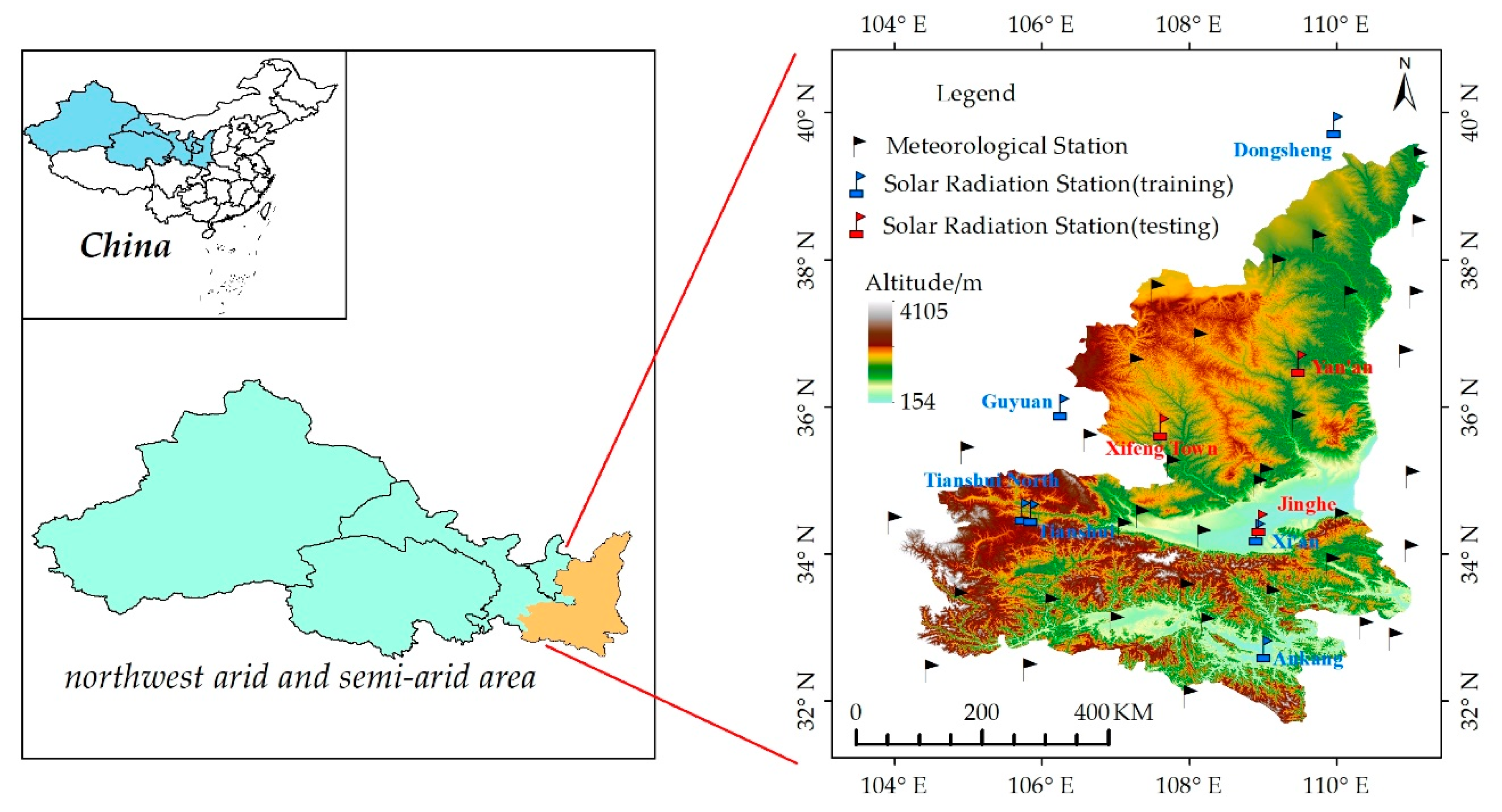
2.1. Data and Test Area

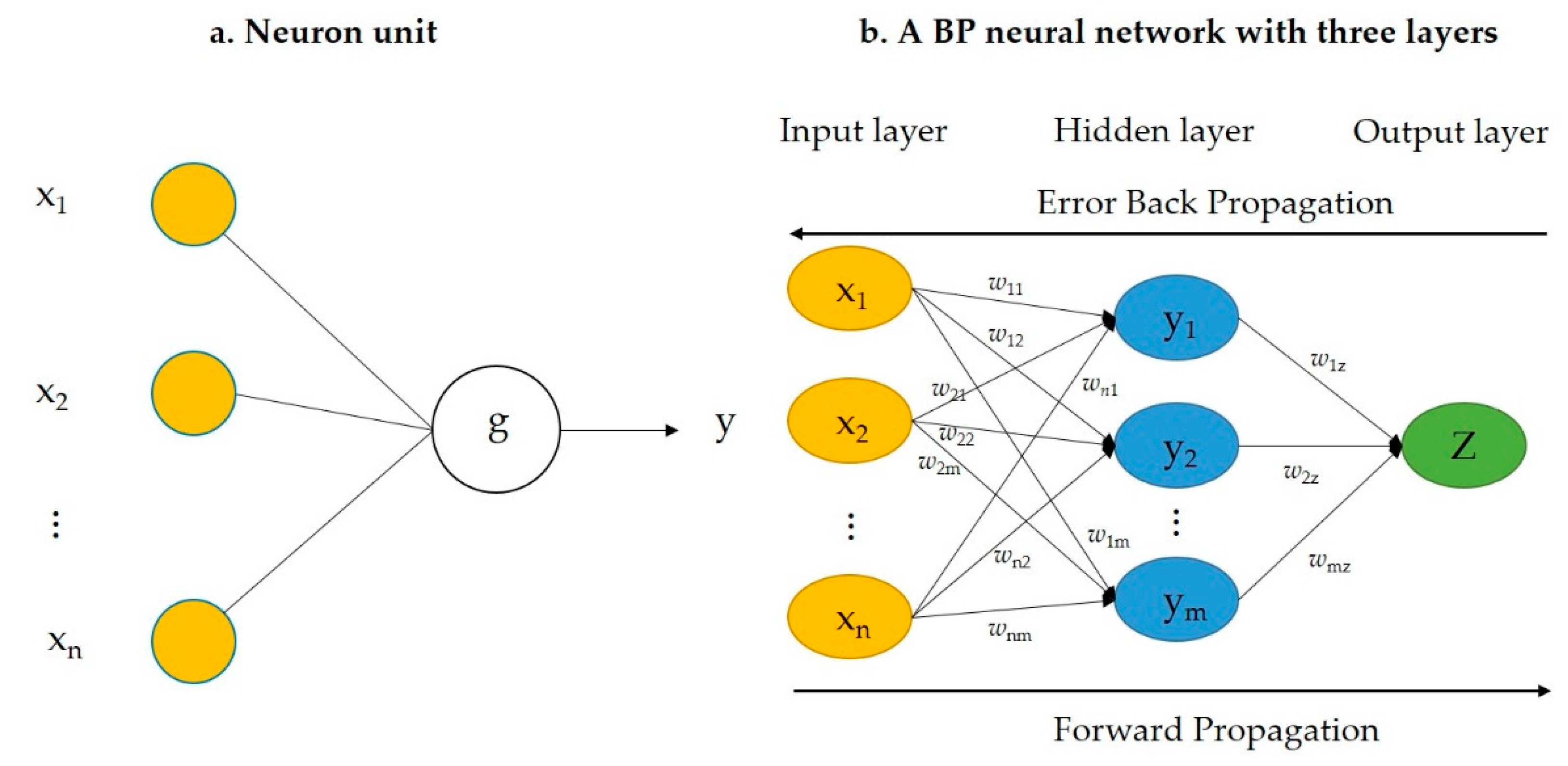
Monthly-averaged AOT, CF, COT and PWV data were extracted from MOD08-M3 atmospheric products aggregated to an equal-angle global grid database. The MOD08-M3 dataset were provided by the earth observing system data and information system (EOSDIS) of the National Aeronautics and Space Administration (NASA) covering the period from January 2001 to December 2013. The monthly-mean values of T, S₀, P, Pw, RH used as the input parameters of the empirical models [13,32,33,34] and observed M-GSR in the same period were provided by the China Meteorological Administration (CMA). Yet, uncertainties in solar radiation measurements may occur, such as instrument mal-functions and occasional voltage instability. Thus, quality control of the solar radiation data was conducted following the work of Tang et al. [35].

After screening remotely sensed data of northwest arid and semi-arid areas of China from 2001 to 2013, we found decent data for Shaanxi and its surrounding areas (Figure 1). So we picked this area as a test area of this study. The terrain is complex, and the precipitation and temperatures vary significantly from the south to the north. Air temperature gradually decreases from the south to north, and the annual average temperature ranges around 7–16 °C; the annual average precipitation is 576.9 mm.

The study area includes nine radiation sites and thirty-six conventional meteorological sites. In this study, six radiation sites (the blue signs in Figure 1), from 2001 to 2013, were used in the training process and the remaining three radiation sites, (the red signs in Figure 1) from 2008 to 2013, were applied in the process of validation; the training and validation stations are distributed over a wide range of latitudes, longitudes, and altitudes in order to ensure a representative estimation algorithm in this study.

2.2 ANN Model

ANN is typically composed of interconnected neuron units organized in layers, it can be applied to recognize patterns, fit a function, and cluster data [36]. In this study, a BP neural network was used to realize the fitting ability of ANN, which is illustrated in Figure 2. On the left panel of this figure, the schematic diagram of a neuron unit was displayed and its function can be mathematically expressed as:

$$y=g({\sum }_{\mathrm{i}-1}^{\mathrm{n}}{w}_i{x}_i)$$

(1)

where i represents the index, xi is one component of the input vector, wi is the weight for each xi, g(·) is the transfer function, which can take many function forms, such as log-sigmoid, tan-sigmoid, and purelin. On the right panel of Figure 2, a BP neural network with three layers containing one input layer, single hidden layer, and one output layer were illustrated; it is a backward propagation of errors [37], the data were propagated from the input layer to the output layer through the hidden layer; while the error was transmitted in the opposite direction, thereby correcting the connection weight (w_nm) of the network. The final error became smaller and smaller. The design of a neural network consists of a transfer function, a training algorithm, a number of hidden layer and a training/test set.

2.3 ANN Implementation

As mentioned in Section 2.2, the ANN implementation comprises several stages:

(1)

Transfer function: the combination of a sigmoid and linear transfer function achieved great simulation results [27,39]. In this work, the tan-sigmoid was a transfer function from the input layer to the hidden layer, and the purelin as transfer function from hidden layer to output layer.

(2)

Learning algorithm: The LM algorithm, a combination of a gradient descent method and Gauss–Newton method [40], were applied in this work. Compared with the Gauss–Newton method, the LM algorithm presents a fast local convergence feature, and it also has the gradient descent method to adjust the weight of each layer, greatly improving the convergence rate and generalization ability of the network. Its learning rule is:

$${x(k+1)=x\left(k\right)-[J}^T{J=\mu I]}^{-1}{J}^{T}e$$

(2)

where e denotes the error vector, J represents the network error of the weights derivative Jacobian matrix, I is the unit matrix, u is a variable and its value determines that the algorithm is based on the Newton’s method or the gradient method. When the coefficient u is zero, the formula is the Newton method; when the value of u is large, the above equation becomes smaller step gradient descent.

(3)

Training/test set: A total of 504 input/output pairs at 6 stations from 2000 to 2013 were used to train ANN to build the relationship between solar radiation and the input vector, and 216 pairs from 2008 to 2013 at the remaining 3 stations (the red points in Figure 1) that were applied in the process of validation.

(4)

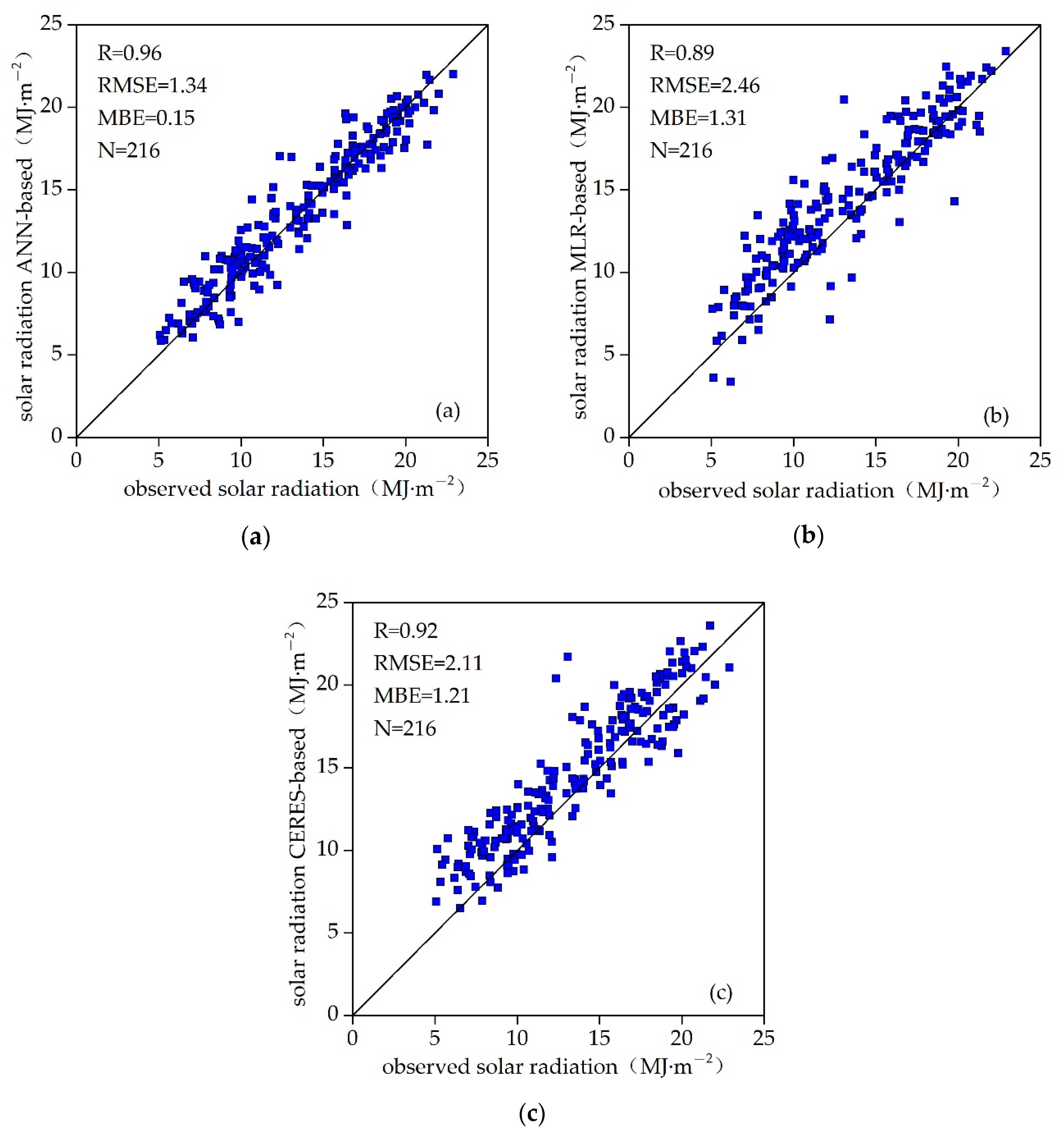
Hidden layer: The design of BP neural network should take the number of neurons in the hidden layer; the number of neurons in the single hidden layer can be calculated by (3).

$$\mathrm{n}=\sqrt{\mathrm{q}+\mathrm{v}}+\mathrm{a}$$

(3)

where q is the number of neurons in the input layer, v the number of neurons in the output layer, a is a the constant, and 1 < a < 10. Different numbers of neurons in the hidden layer were tested in order to select a relatively optimized network structure. After training, a comparison was performed between simulated M-GSR and observed ones at the training sites. R, RMSE and MBE were used as error metrics for comparison; these statistics are defined as follows:

$$\mathrm{R}=\frac{{\sum }_{i=1}^{\mathrm{N}}({\mathrm{x}}_{\mathrm{i}}-\overline{\mathrm{x}})({\mathrm{y}}_{\mathrm{i}}-\overline{\mathrm{y}})}{\sqrt{{\sum }_{i=1}^{\mathrm{N}}{({\mathrm{x}}_{\mathrm{i}}-\overline{\mathrm{x}})}^2}\sqrt{{\sum }_{i=1}^{\mathrm{N}}{({\mathrm{y}}_{\mathrm{i}}-\overline{\mathrm{y}})}^2}}$$

(4)

$$\mathrm{RMSE}=\sqrt{{\sum }_{\mathrm{i}=1}^{\mathrm{N}}{{(\mathrm{H}}_{\mathrm{e}}{-\mathrm{H}}_{\mathrm{m}})}^2/\mathrm{N}}$$

(5)

$$\mathrm{MBE}={\sum }_{\mathrm{i}=1}^{\mathrm{N}}{(\mathrm{H}}_{\mathrm{e}}{-\mathrm{H}}_{\mathrm{m}})/\mathrm{N}$$

(6)

where H_e the estimated M-GSR, and H_m the measured M-GSR, and N the number of samples. If RMSE and MBE are smaller, the simulation precision is higher. The performance of the number of neurons in hidden layer is shown in

Table 1. Training results for different configurations in the hidden layer.

n	Transfer Function		Training Function	R	RMSE/ MJ·m−2	MBE/ MJ·m−2
	Hidden Layer	Output Layer
4	tan-sigmoid	purelin	trainlm	0.94	1.59	0.13
5	tan-sigmoid	purelin	trainlm	0.93	1.66	0.12
6	tan-sigmoid	purelin	trainlm	0.94	1.60	0.44
7	tan-sigmoid	purelin	trainlm	0.96	1.34	0.21
8	tan-sigmoid	purelin	trainlm	0.93	1.65	0.27
9	tan-sigmoid	purelin	trainlm	0.92	2.12	1.15
10	tan-sigmoid	purelin	trainlm	0.94	1.66	0.52
11	tan-sigmoid	purelin	trainlm	0.90	1.99	0.42
12	tan-sigmoid	purelin	trainlm	0.92	1.76	0.19
13	tan-sigmoid	purelin	trainlm	0.93	1.73	0.20

. When the ANN configuration is with 7 neurons in the hidden layer, the value of RMSE is the smallest and the value of R is optimal (RMSE = 1.34 MJ·m⁻², with R = 0.96). MBE is minimum (equal to 0.12 MJ·m⁻²) when the ANN configuration with 5 neurons in the hidden layer. It is indicated that the training results were hardly improved further when the number of neurons in the hidden layer became greater than 7. The more the number of neurons, the not higher the accuracy. The reason is that the more the number of hidden layers, the more the nodes, which leads to more weights and errors, hence, the accuracy of the network drops. From the above consideration, an ANN configuration with 7 neurons was applied.

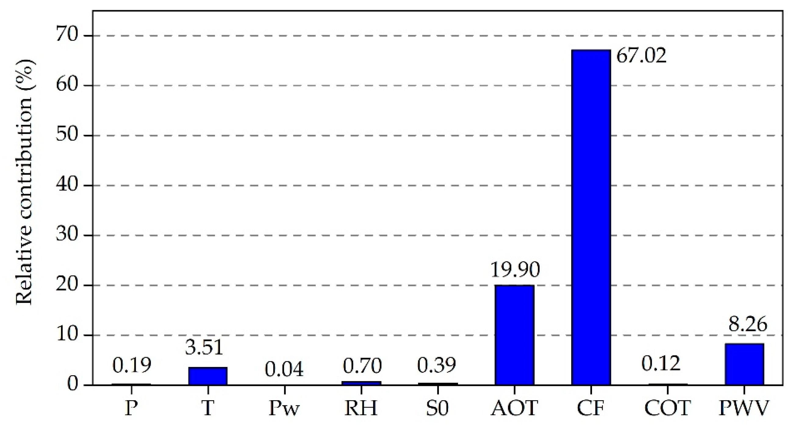
2.4. Contribution Assessment

In this study, a multiple regression analysis was used to assess the contribution of input variables to the output [41]. The proportion of one variable’s regression coefficient accounts for the sum of all variables’ regression coefficients and represents the relative contribution of the changes of the variable to solar radiation:

$$\mathrm{y}={\mathrm{m}}_1{\mathrm{x}}_1{+\mathrm{m}}_2{\mathrm{x}}_2{+\mathrm{m}}_3{\mathrm{x}}_3+\dots$$

(7)

$${\mathrm{s}}_1=\frac{\left|{\mathrm{m}}_1\right|}{\left|{\mathrm{m}}_1\right|+\left|{\mathrm{m}}_2\right|+\dots +\left|{\mathrm{m}}_{\mathrm{j}}\right|}$$

(8)

where y is the M-GSR, x₁, x₂, x₃ … are the values of first, second, third … meteorological factors, m₁, m₂, m₃ are the regression coefficients for first, second, third … meteorological factors, and s₁ is the relative contribution of the variation of x₁ to M-GSR. According to Figure 3, of the 10 variables, CF has the greatest contribution to solar radiation in Shaanxi Province and its surrounding areas, followed by AOT, PWV. Other variables have less influence on solar radiation. Peng et al. [42] analyzed the variation of solar radiation and its impact factors of Xi’an city, Shaanxi province in recent 50 years, they pointed out that clouds and aerosols play a major role in reducing solar radiation reaching the surface. In this study, clouds, aerosols and predictable water vapor were considered first. Then, the meteorological variables (P, T, Pw, RH and S₀) as the first group (hereafter ‘ANN1’); at the same time, CF, AOT, PWV and PWV along with the meteorological variables as the second group of input parameters to simulate solar radiation (hereafter ‘ANN2’). From results, the estimated value of ANN2 was found to be closer to the observations (Figure 4).

Table 2. Comparison of ANN1 and ANN2.

ANN with Different Inputs	RMSE/MJ·m−2	MBE/MJ·m−2	R
ANN1	2.31	−1.13	0.89
ANN2	1.34	0.15	0.96

gives out different statistics for ANN1 and ANN2. The statistical results show that the ANN2 model outperforms significantly ANN1 (Table 2). It demonstrates that clouds, aerosols, and precipitation water vapor are the most important factors affecting solar radiation changes in Shaanxi and its surrounding areas.

3. Results and Discussion

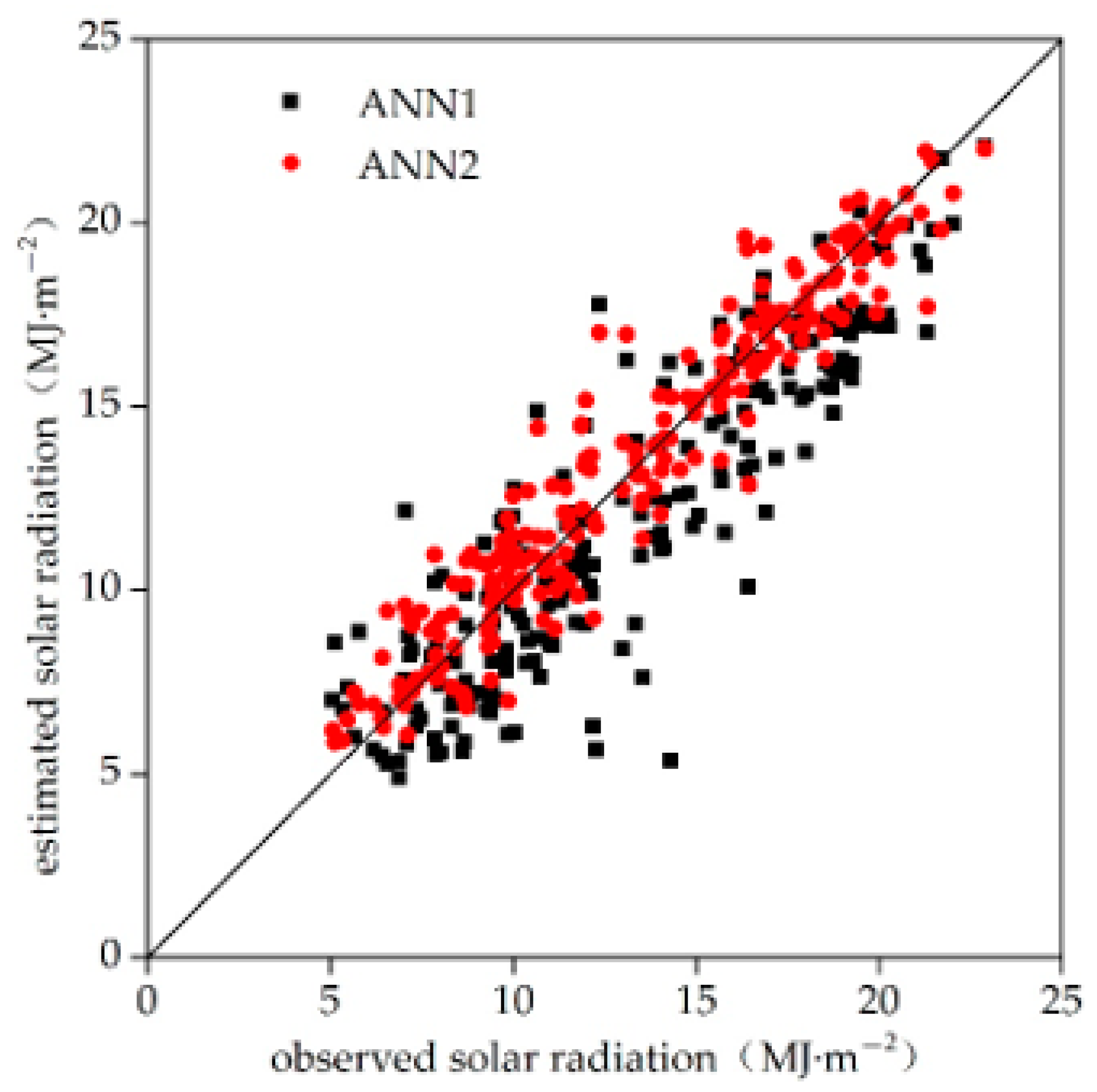
3.1. Performances of ANN Model

The ANN method should be evaluated at sites where solar radiation data were not used in the training process. Moreover, the ANN-based solar radiation model also needed a comparison with estimation methods and existing satellite products. So estimates derived from the MLR model and the CERES monthly-mean daily solar radiation product with a spatial resolution of 1° were chosen in this study. The reason for choosing the MLR and CERES radiation products was: The use of the same input parameters in the MLR and ANN-based models, thereby avoiding inconsistencies in input parameters, while CERES has been currently considered to be relatively highly accurate [43]. Figure 5 shows the comparison between measured and estimated M-GSR from the ANN model, the MLR method and the CRERS radiation product; correlation coefficient (R) for ANN-based model is 0.96, while that for the MLR method and CRERS radiation product is 0.89 and 0.92, respectively; and the values of RMSE were 1.34 MJ·m⁻², 2.46 MJ·m⁻², 2.11 MJ·m⁻², respectively. It shows that the ANN-based and the MLR models have better ability of simulation, and the CRERS radiation product has a relatively high accuarcy.

In order to further investigate the performance of the ANN algorithm in this study, the solar radiation data serve for each validation site was plotted and error metrics were provided. As seen in Figure 6, the estimates of the three methods are consistent with the overall trend of the observations, but the performance is different at each of the 3 validation sites, that is possibility because of the heterogeneity over the rugged terrain [14,44]. Jinghe is located in the Guanzhong plain, Xifeng Town is located in the gully region of the Loess Plateau, and Yan’an is within hilly and gully region of the Loess Plateau. The annual error of the 3 methods for the 3 sites were calculated, as shown in

Table 3. Statistical indicators of the models and CERES.

Station	Year	RMSE(MJ·m−2)			MBE(MJ·m−2)			R
		CERES	ANN	MLR	CERES	ANN	MLR	CERES	ANN	MLR
Yan’an	2008	1.67	0.56	1.81	1.60	0.01	0.70	0.99	0.99	0.93
	2009	1.70	1.28	1.32	1.64	−0.45	0.80	0.99	0.96	0.97
	2010	1.57	1.05	1.16	1.44	−0.34	0.08	0.99	0.97	0.97
	2011	1.35	1.40	1.05	1.28	−0.41	0.37	0.99	0.96	0.98
	2012	1.82	0.91	1.19	1.69	−0.50	0.40	0.99	0.98	0.97
	2013	3.99	2.35	2.97	2.36	1.36	1.53	0.65	0.88	0.76
	Mean	2.02	1.25	1.58	1.67	−0.05	0.65	0.93	0.96	0.93
Xifeng Town	2008	2.34	1.05	2.07	1.82	0.16	−0.36	0.95	0.98	0.91
	2009	2.88	1.42	2.51	2.22	0.96	−0.24	0.92	0.99	0.86
	2010	3.09	1.48	2.32	2.76	1.20	2.01	0.90	0.96	0.94
	2011	2.67	1.37	3.03	2.49	1.03	2.88	0.98	0.98	0.98
	2012	2.62	0.97	1.88	2.20	−0.19	1.13	0.96	0.98	0.97
	2013	2.30	1.18	2.25	2.04	0.25	1.84	0.97	0.96	0.96
	Mean	2.65	1.25	2.34	2.26	0.57	1.24	0.95	0.98	0.94
Jinghe	2008	1.38	1.56	2.06	−1.04	−0.80	0.31	0.98	0.97	0.89
	2009	1.30	1.53	2.49	−0.16	−0.58	1.90	0.97	0.97	0.96
	2010	0.90	1.19	2.63	0.45	0.22	2.17	0.97	0.93	0.88
	2011	1.11	1.23	1.55	−0.74	−1.06	1.36	0.99	0.99	0.99
	2012	1.10	1.00	1.38	−0.91	−0.04	0.70	0.99	0.98	0.97
	2013	1.44	1.75	2.32	−0.86	0.89	1.34	0.96	0.94	0.92
	Mean	1.21	1.38	2.07	−0.54	−0.23	1.30	0.98	0.96	0.94

. The RMSE values of the ANN-based model and the MLR method are 0.56~2.35 MJ·m⁻² and 1.05~3.03 MJ·m⁻² at the 3 sites, respectively; the MBE values are −1.06~1.36 MJ·m⁻² and −0.36~2.88 MJ·m⁻²; the R values are 0.93~0.99 and 0.76~0.99, respectively. Compared to the ANN-based model, the CERES retrieval radiation products have a slightly lower precision (the RMSE values are from 0.9 to 3.99 MJ·m⁻²; the MBE values are from −1.04 to 2.76 MJ·m⁻²; the R values between 0.65 and 0.99), probably due to some uncertainties influencing the accuracy of the CERES radiation products, such as the error of remote sensor, the error of the algorithm itself, and the error of parameter estimation in the algorithm [45]. In summary, The ANN-based method has a relatively high estimation accuracy and stability.

3.2. Comparison with Models from the Literature

In order to verify the effectiveness of the M-GSR prediction model of our study with AOT, CF, COT, PWV parameters, we made a comparison with other published M-GSR models, as shown in

Table 4. Comparison between various monthly mean daily global solar radiation models.

Model	Input Parameters	Location	Author/Ref.	R	MBE/ MJ·m−2	RMSE/ MJ·m−2
ANN	LST, DT, Precipitation, EVI, DOY, τ	Tibetan plateau/ China	Qin [46]	0.89~0.99	-	0.86~1.85
	ANN-S: S0, day length ANN-T: Tmax, Tmin ANN-ST: S0, day length, Tmax, Tmin	Tamil Nadu, India	Meenal [47]	0.92~0.98 0.77~0.93 0.94~0.98	0.02~0.66 −0.14~0.33 −0.03~0.48	0.75~1.45 0.89~2.22 0.58~1.18
	T, Precipitation, RH, P, S0, Tmax, Tmin, Latitude, Longitude, Altitude	Southeast/ China	Zou [48]	0.93~0.97	-	-
	Latitude, Longitude, Altitude, Year, Month, T, P, Wind speed, RH	Munbai, India	Premalatha [49]	-	-	3.65
	LST, Latitude, Longitude, Altitude, Months	Austrlia	Deo [19]	0.90~0.98	-	0.93~1.85
	Month, Latitude, Longitude, Altitude, Tmin, RH, Tmax, Bright Sunshine, Wind Speed, CF	Bangladesh	Abedin [1]	0.83	-	-
	LM-BP: AOT, CF, COT, PWV, T, S0, P, Pw, RH	Shaanxi/China	Our study	0.93~0.99	0.15	1.34
Empirical model	Hargreaves-Samani: Tmax, Tmin	Mexico	Rivero [13]	0.57~0.77	-	2.86~3.63
	Empirical model: S, S0, H0	China	Chen [32]	-	1.98~2.7	-
	Bristow and Campbell: Tmax, Tmin	China	Chen [33]	-	1.51	-
	Abdalla model: H0, S0, RH, T	Turkey	Citakoglu [34]	0.91	43.95	-
	MLR: AOT, CF, COT, PWV, T, S0, P, Pw, RH	Shaanxi/China	Our study	0.76~0.99	1.31	2.46

. The comparison was carried out in terms of statistical performance metrics namely R, MBE, and RMSE. All the ANN-based models had a good performace. But the performance of the ANN models, with different input parameters, was unequal as reported in Table 4. Qin et al. [46] considered the land surface temperature (LST), the DT, the precipitation, the Enhanced Vegetation Index (EVI), the day of the year (DOY), the transmissivity (τ), and had better results (R ranged between 0.89 and 0.99). In a Meenal article [47], S₀ and T were used as input to predict M-GSR; the results showed that when the two were combined as input parameters, the simulation accuracy was the highest (R ranged from 0.94 to 0.99). Although Abedin et al. [1] considered CF when simulating solar radiation, the value of R was only 0.83. The possible reason was that the effects of AOT and PWV were not considered at the same time. It can be clearly noticed that the LM-BP model developed in our study with AOT, CF, COT, PWV parameters achieved better outcomes (RMSE and MBE of 1.34 MJ·m⁻², 0.15 MJ·m⁻², respectively) than the other ANN models listed in the literature [1,19,46,47,48,49]. With reference to Table 4, it can be seen that all empirical models [13,33,34] use temperature and sunshine hours as the main input parameters to estimate M-GSR. These empirical models have low performance compared with our MLR model, especially the Hargreaves-Samani model with Tmin and Tmax as the main parameters. Hence, it is demonstrated that the influencing parametets namely aerosols, clouds and perceptible water vapor play a major role in obtaining a good prediction accuracy of M-GSR. Also, the ANN with the LM-BP algorithm, and with input parameters of AOT, CF, COT, PWV, can be applied to estimate solar radiation on the surface efficiently and effectively.

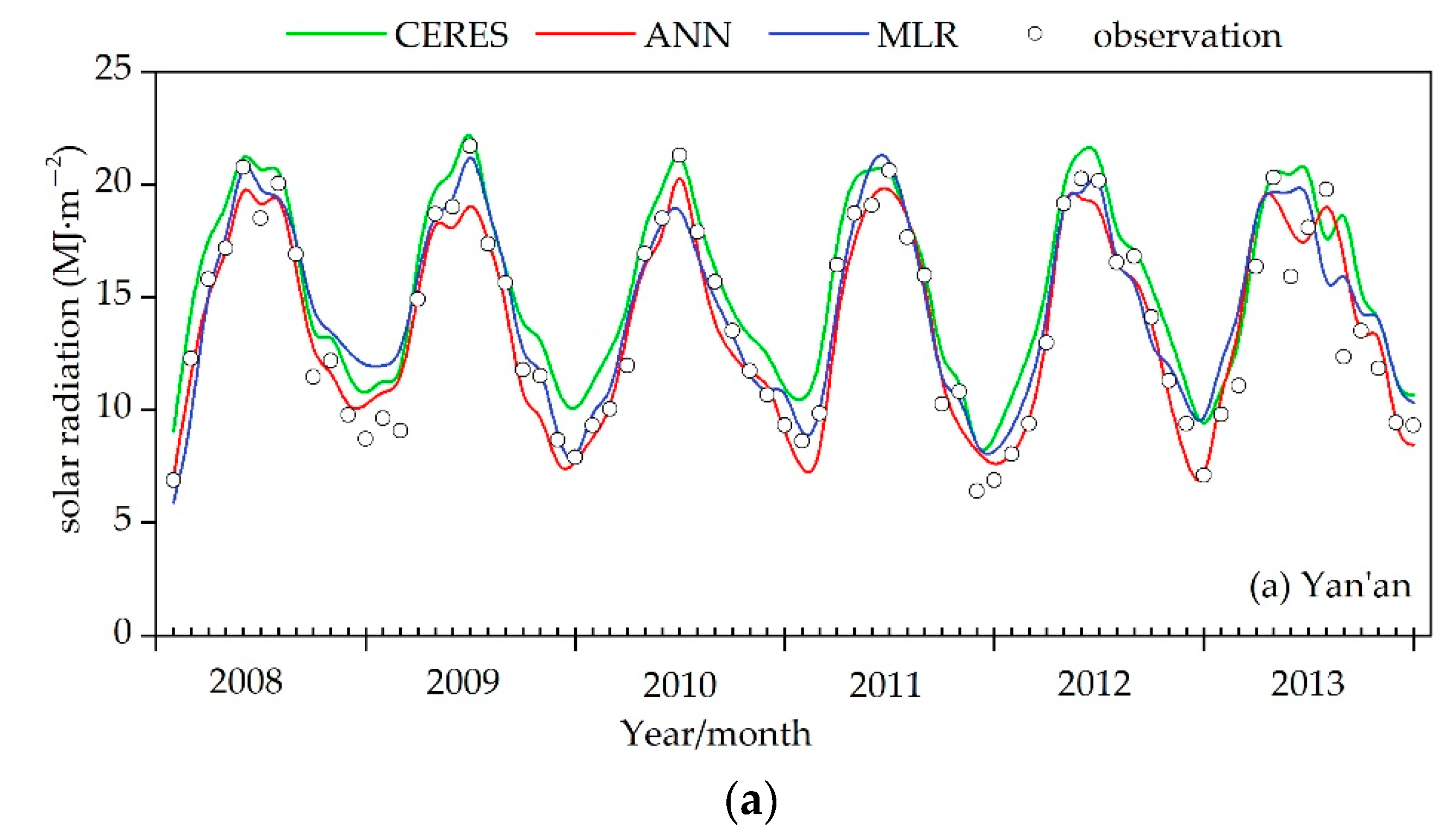
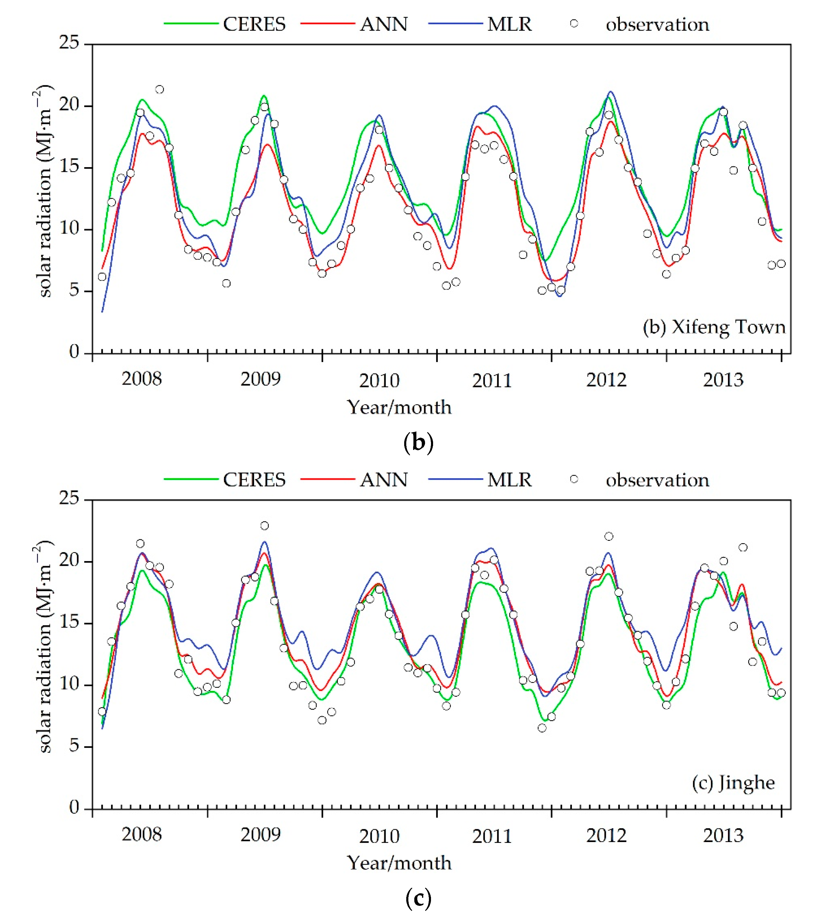
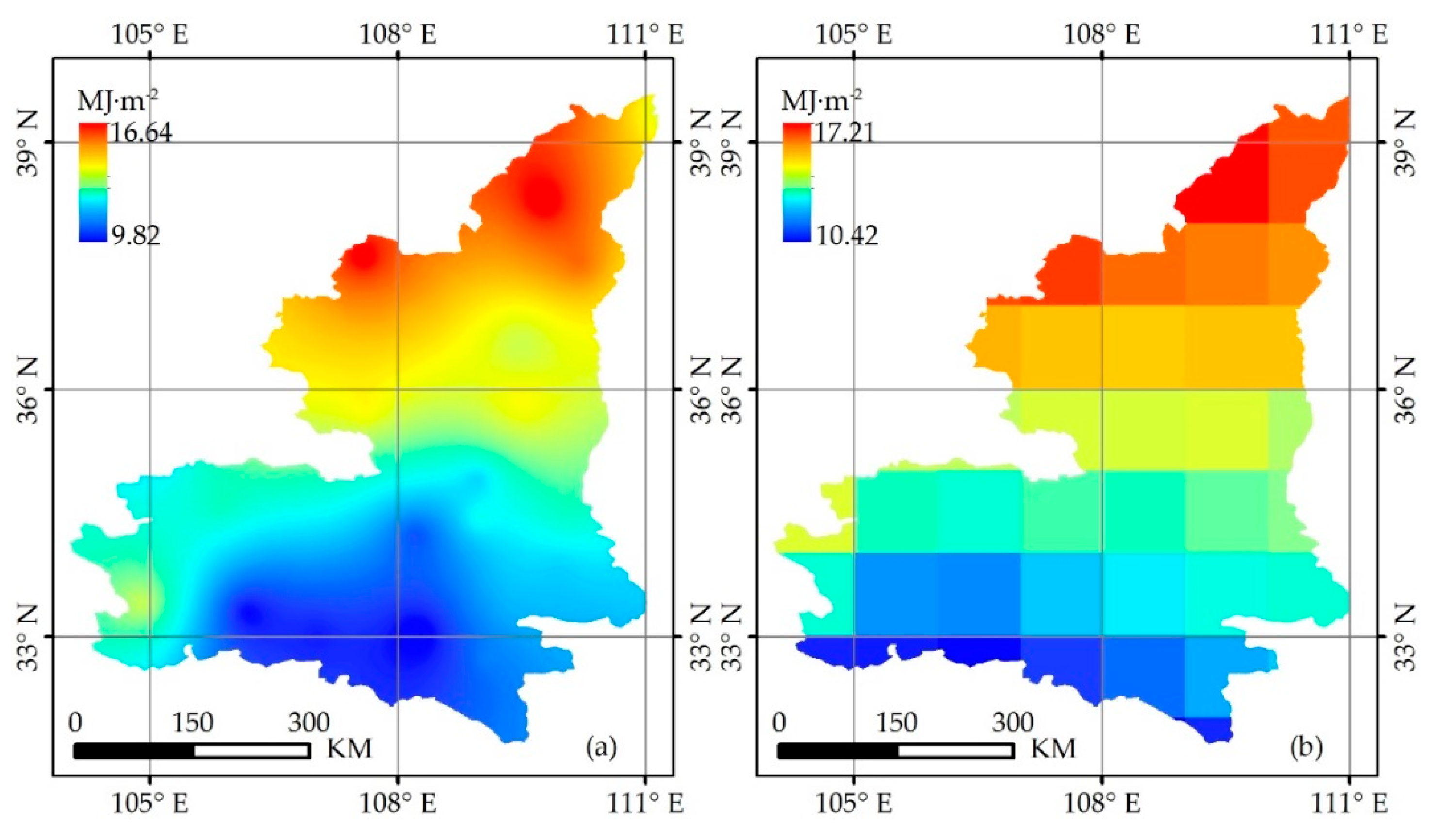
3.3. Receiving Regional Monthly Mean Solar Radiation

According to the established ANN-based method, the M-GSR at 36 conventional meteorological stations for 12 months, was estimated in 2012 in Shaanxi Province and its surrounding regions. Then, spatial distribution of the solar radiation was obtained with the simulated values and observations, with a spatial resolution of 1 km (Figure 7a). As seen, these images thoroughly exhibit the spatial patterns of solar radiation over Shaanxi Province and its surrounding regions. The solar radiation values in the north are much larger than those in the south. This is mainly because the southern Shaanxi Province belongs to the Qinba Mountain area, the vegetation coverage is high and the air is relatively humid. The absorption of solar radiation is stronger in these areas, and, therefore, the solar radiation on the surface is relatively low. To the contrary, the northern Shaanxi Province belongs to the Loess Plateau, where the situation is just the opposite of the south; the solar radiation on the surface is relatively high. At the same time, comparing the interpolated solar radiation with the CERES product (spatial resolution of 1°), shows that the spatial distribution of solar radiation, obtained by the two methods, is similar, but the ANN-based solar radiation is finer (Figure 7).

4. Conclusions

In this work, the BP neural network based on the LM algorithm, having been developed namely cloud, aerosol, and perceptible water vapor data from MODIS along with conventional meteorological data, was applied to estimate the monthly-mean daily global solar radiation in Shaanxi Province and its surroundings. This work took neural network into consideration, and showed that the ANN configuration with seven neurons in the hidden layer was excellent. The contribution assessment demonstrated that the cloud, aerosol, and precipitation water vapor are the most important factors affecting solar radiation changes in Shaanxi and its surrounding areas. Comparisons were carried out among the ANN-based model, the MLR model, and the remotely-sensed radiation products by CERES, and showed that this ANN-based method can obtain monthly-mean daily global solar radiation with high accuracy (R = 0.96, RMSE = 1.34 MJ·m⁻², MBE = 0.15 MJ·m⁻²) and good stability.

In summary, the following findings were obtained in this work. First, the ANN-based model with clouds, aerosols, and precipitable water vapor was accurate and effective to predict the monthly-mean daily solar radiation for the locations where there are limited observations. Second, clouds, aerosols, and precipitation water vapor play a very important role in obtaining highly accurate results of solar radiation. In the future, the LM-BP neural network method presented in this study can be used to obtain the daily scale and even higher time resolution spatial solar radiation to allow people to make full use of solar energy resources. Additionally, the components of global solar radiation, that is, scattered radiation and direct radiation, are closely related to clouds, aerosols, and water vapor. In future work, the estimation method in this study developed with clouds, aerosols, and water vapor can couple with other datasets to estimate scattered radiation and direct radiation to get more accurate global solar radiation.

References

1. Abedin, Z.; Barua, M.; Paul, S.; Akther, S.; Chowdhury, R.; Chowdhury, M. A model for prediction of monthly solar radiation of different meteorological locations of Bangladesh using artificial neural network data mining tool. In Proceedings of the 2017 International Conference on Electrical, Computer and Communication Engineering (ECCE), Cox’s Bazar, Bangladesh, 16–18 February 2017; pp. 692–697. [Google Scholar]
2. Wang, D.; Liang, S.; He, T. Mapping high-resolution surface shortwave net radiation from landsat data. IEEE Geosci. Remote Sens. Lett. 2014, 11, 459–463. [Google Scholar] [CrossRef]
3. Gairaa, K.; Khellaf, A.; Messlem, Y.; Chellali, F. Estimation of the daily global solar radiation based on box–jenkins and ann models: A combined approach. Renew. Sustain. Energy Rev. 2016, 57, 238–249. [Google Scholar] [CrossRef]
4. Rabehi, A.; Guermoui, M.; Lalmi, D. Hybrid models for global solar radiation prediction: A case study. Int. J. Ambient Energy 2018, 1–10. [Google Scholar] [CrossRef]
5. Angstrom, A. Solar and terrestrial radiation. Report to the international commission for solar research on actinometric investigations of solar and atmospheric radiation. Q. J. R. Meteorol. Soc. 1924, 50, 121–126. [Google Scholar] [CrossRef]
6. Valiantzas, J.D. Modification of the hargreaves–samani model for estimating solar radiation from temperature and humidity data. J. Irrig. Drain. Eng. 2018, 144. [Google Scholar] [CrossRef]
7. Kambezidis, H.D.; Psiloglou, B.E.; Karagiannis, D.; Dumka, U.C.; Kaskaoutis, D.G. Meteorological Radiation Model (MRM V 6.1): Improvements in diffuse radiation estimates and a new approach for implementation of cloud products. Renew. Sustain. Energy Rev. 2017, 74, 616–637. [Google Scholar] [CrossRef]
8. Bristow, K.L.; Campbell, G.S. On the relationship between incoming solar radiation and daily maximum and minimum temperature. Agric. For. Meteorol. 1984, 31, 159–166. [Google Scholar] [CrossRef]
9. Akinoğlu, B.G.; Ecevit, A. A further comparison and discussion of sunshine-based models to estimate global solar radiation. Energy 1990, 15, 865–872. [Google Scholar] [CrossRef]
10. Louche, A.; Notton, G.; Poggi, P.; Simonnot, G. Correlations for direct normal and global horizontal irradiation on a French Mediterranean site. Sol. Energy 1991, 46, 261–266. [Google Scholar] [CrossRef]
11. Barker, H.W.; Cole, J.; Li, J.N. Application of Monte Carlo solar radiative transfer model in the McICA framework. Q. J. R. Meterorol. Soc. 2015, 141, 3130–3139. [Google Scholar] [CrossRef]
12. Da Silva, M.B.P.; Francisco Escobedo, J.; Juliana Rossi, T.; dos Santos, C.M.; da Silva, S.H.M.G. Performance of the Angstrom-Prescott model (A-P) and SVM and ANN techniques to estimate daily global solar irradiation in botucatu/sp/brazil. J. Atmos. Sol. Terr. Phys. 2017, 160, 11–23. [Google Scholar] [CrossRef]
13. Rivero, M.; Orozco, S.; Sellschopp, F.S.; Loera-Palomo, R. A new methodology to extend the validity of the Hargreaves-Samani model to estimate global solar radiation in different climates: Case study mexico. Renew. Energy 2017, 114, 1340–1352. [Google Scholar] [CrossRef]
14. Zhang, Y.; Li, X.; Bai, Y. An integrated approach to estimate shortwave solar radiation on clear-sky days in rugged terrain using modis atmospheric products. Sol. Energy 2015, 113, 347–357. [Google Scholar] [CrossRef]
15. Moustris, K.; Paliatsos, A.G.; Bloutsos, A.; Nikolaidis, K.; Koronaki, I.; Kavadias, K. Use of neural networks for the creation of hourly global and diffuse solar irradiance data at representative locations in Greece. Renew. Energy 2008, 33, 928–932. [Google Scholar] [CrossRef]
16. Behrang, M.A.; Assareh, E.; Ghanbarzadeh, A.; Noghrehabadi, A.R. The potential of different artificial neural network (ANN) techniques in daily global solar radiation modeling based on meteorological data. Sol. Energy 2010, 84, 1468–1480. [Google Scholar] [CrossRef]
17. Ramedani, Z.; Omid, M.; Keyhani, A. Modeling solar energy potential in a tehran province using artificial neural networks. Int. J. Green Energy 2013, 10, 427–441. [Google Scholar] [CrossRef]
18. Waewsak, J.; Chancham, C.; Mani, M.; Gagnon, Y. Estimation of monthly mean daily global solar radiation over bangkok, thailand using artificial neural networks. Energy Procedia 2014, 57, 1160–1168. [Google Scholar] [CrossRef]
19. Deo, R.C.; Şahin, M. Forecasting long-term global solar radiation with an ann algorithm coupled with satellite-derived (MODIS) land surface temperature (LST) for regional locations in queensland. Renew. Sustain. Energy Rev. 2017, 72, 828–848. [Google Scholar] [CrossRef]
20. Rehman, S.; Mohandes, M. Artificial neural network estimation of global solar radiation using air temperature and relative humidity. Energy Policy 2008, 36, 571–576. [Google Scholar] [CrossRef] [Green Version]
21. Rao, K.D.V.S.K.; Premalatha, M.; Naveen, C. Analysis of different combinations of meteorological parameters in predicting the horizontal global solar radiation with ANN approach: A case study. Renew. Sustain. Energy Rev. 2018, 91, 248–258. [Google Scholar] [CrossRef]
22. Teke, A.; Yıldırım, H.B.; Çelik, Ö. Evaluation and performance comparison of different models for the estimation of solar radiation. Renew. Sustain. Energy Rev. 2015, 50, 1097–1107. [Google Scholar] [CrossRef]
23. Wang, L.; Kisi, O.; Zounemat-Kermani, M.; Salazar, G.A.; Zhu, Z.; Gong, W. Solar radiation prediction using different techniques: Model evaluation and comparison. Renew. Sustain. Energy Rev. 2016, 61, 384–397. [Google Scholar] [CrossRef]
24. Mubiru, J.; Banda, E.J.K.B. Estimation of monthly average daily global solar irradiation using artificial neural networks. Sol. Energy 2008, 82, 181–187. [Google Scholar] [CrossRef]
25. Lam, J.C.; Wan, K.K.W.; Yang, L. Solar radiation modelling using ANNs for different climates in China. Energy Convers. Manag. 2008, 49, 1080–1090. [Google Scholar] [CrossRef]
26. Wang, Z.; Wang, F.; Su, S. Solar irradiance short-term prediction model based on bp neural network. Energy Procedia 2011, 12, 488–494. [Google Scholar] [CrossRef]
27. Notton, G.; Paoli, C.; Vasileva, S.; Nivet, M.L.; Canaletti, J.-L.; Cristofari, C. Estimation of hourly global solar irradiation on tilted planes from horizontal one using artificial neural networks. Energy 2012, 39, 166–179. [Google Scholar] [CrossRef]
28. Yadav, A.K.; Malik, H.; Chandel, S.S. Selection of most relevant input parameters using WEKA for artificial neural network based solar radiation prediction models. Renew. Sustain. Energy Rev. 2014, 31, 509–519. [Google Scholar] [CrossRef]
29. Vakili, M.; Sabbagh-Yazdi, S.-R.; Kalhor, K.; Khosrojerdi, S. Using artificial neural networks for prediction of global solar radiation in tehran considering particulate matter air pollution. Energy Procedia 2015, 74, 1205–1212. [Google Scholar] [CrossRef]
30. Kashyap, Y.; Bansal, A.; Sao, A.K. Solar radiation forecasting with multiple parameters neural networks. Renew. Sustain. Energy Rev. 2015, 49, 825–835. [Google Scholar] [CrossRef]
31. Rossow, W.B.; Zhang, Y. Calculation of surface and top of atmosphere radiative fluxes from physical quantities based on ISCCP data sets: 2. Validation and first results. J. Geophys. Res. Atmos. 1995, 100, 1167–1197. [Google Scholar] [CrossRef]
32. Chen, J.L.; Li, G.S.; Wu, S.J. Assessing the potential of support vector machine for estimating daily solar radiation using sunshine duration. Energy Convers. Manag. 2013, 75, 311–318. [Google Scholar] [CrossRef]
33. Chen, J.L.; Liu, H.B.; Wu, W.; Xie, D.-T. Estimation of monthly solar radiation from measured temperatures using support vector machines—A case study. Renew. Energy 2011, 36, 413–420. [Google Scholar] [CrossRef]
34. Citakoglu, H. Comparison of artificial intelligence techniques via empirical equations for prediction of solar radiation. Comput. Electron. Agric. 2015, 118, 28–37. [Google Scholar] [CrossRef]
35. Tang, W.; Yang, K.; He, J.; Qin, J. Quality control and estimation of global solar radiation in China. Sol. Energy 2010, 84, 466–475. [Google Scholar] [CrossRef]
36. Demuth, H.; Beale, M.; Hagan, M. Neural Network Toolbox 6: Users Guide; Mathwork Inc.: Natick, MA, USA, 2008; Volume 21, pp. 1225–1233. [Google Scholar]
37. Mosavi, M.R.; Khishe, M. Training a feed-forward neural network using particle swarm optimizer with autonomous groups for sonar target classification. J. Circuits Syst. Comput. 2017, 26, 1750185. [Google Scholar] [CrossRef]
38. Li, J.; Wang, D.; Feng, J.J. Simulation of solar radiation based on neural network and MODIS remote sensing products. Sci. Geogr. Sin. 2017, 37, 912–919, (In Chinese with English Abstract). [Google Scholar]
39. Krishnaiah, K.; Rao, S.S.; Madhumurthy, K.; Reddy, K.S. Neural network approach for modelling global solar radiation. J. Appl. Sci. Res. 2007, 3, 1105–1111. [Google Scholar]
40. Last, M. Kernel Methods for Pattern Analysis; China Machine Press: Beijing, China, 2005. (In Chinese) [Google Scholar]
41. Pryor, S.C.; Ledolter, J. Addendum to “wind speed trends over the contiguous united states”. J. Geophys. Res. 2010, 115, 10103. [Google Scholar] [CrossRef]
42. Peng, Y.; Wang, Z.; Li, X.; Jin, Y. Variation of surface solar radiation and its impact factors of Xi’an city, Shaanxi province in recent 50 years. Arid. Land Geogr. (Chin.) 2012, 35, 738–745. [Google Scholar]
43. Li, J.; Wang, D. A comparative study on three types of remote sensing solar radiation products. Clim. Environ. Res. 2018, 23, 252–258, (In Chinese with English Abstract). [Google Scholar]
44. Wu, S.; Wen, J.; You, D.; Zhang, H.; Xiao, Q.; Liu, Q. Algorithms for calculating topographic parameters and their uncertainties in downward surface solar radiation (DSSR) estimation. IEEE Geosci. Remote Sens. Lett. 2018, 15, 1149–1153. [Google Scholar] [CrossRef]
45. Liang, S.; Wang, K.; Zhang, X.; Wild, M. Review on estimation of land surface radiation and energy budgets from ground measurement, remote sensing and model simulations. IEEE J. Sel. Top. Appl. Earth Obs. Remote Sens. 2010, 3, 225–240. [Google Scholar] [CrossRef]
46. Qin, J.; Chen, Z.; Yang, K.; Liang, S.; Tang, W. Estimation of monthly-mean daily global solar radiation based on MODIS and TRMM products. Appl. Energy 2011, 88, 2480–2489. [Google Scholar] [CrossRef]
47. Meenal, R.; Selvakumar, A.I. Assessment of svm, empirical and ann based solar radiation prediction models with most influencing input parameters. Renew. Energy 2018, 121, 324–343. [Google Scholar] [CrossRef]
48. Zou, L.; Lin, A.W.; Wang, L.C.; Yang, Q.; Zhao, Z.Z. Monthly mean global solar radiation modeling using artificial neural network technique in southeast hill areas, China during 1993–2003. Energy Mech. Eng. 2016, 394–401. [Google Scholar] [CrossRef]
49. Premalatha, N.; Valan Arasu, A. Prediction of solar radiation for solar systems by using ANN models with different back propagation algorithms. J. Appl. Res. Technol. 2016, 14, 206–214. [Google Scholar] [CrossRef]
Figure 1. Location of the study area.
Energies 11 03510 g001
Figure 2. Neural network interpretation diagram. (a) is a schematic diagram of a neural unit; (b) is a BP neural network with the three layers [38].
Energies 11 03510 g002
Figure 3. Relative contribution of the parameters.
Energies 11 03510 g003
Figure 4. Scatter plot of estimated solar radiation and observations. ANN1 indicates the input parameters of P, T, Pw, RH and S0. ANN2 indicates that the input parameters of P, T, Pw, RH, S0, AOT, CF, COT and PWV.
Energies 11 03510 g004
Figure 5. Comparison between observed solar radiation and simulated values after training at the training stations. (ac) are scatter plots of observed solar radiation and simulated solar radiation based on ANN method, MLR model and CERES products, respectively.
Energies 11 03510 g005
Figure 6. Individual results for 3 validation sites. (a), (b) and (c) are the results of three methods (ANN model, MLR method and CERES radiation products) for Yan’an, Xifeng town and Jinghe, respectively.
Energies 11 03510 g006aEnergies 11 03510 g006b
Figure 7. Spatial distribution of solar radiation in 2012. (a) Solar radiation based on the ANN model, (b) Remotely-sensed radiation product from CERES.
Energies 11 03510 g007