Torque Distribution Algorithm for an Independently Driven Electric Vehicle Using a Fuzzy Control Method: Driving Stability and Efficiency

Abstract

In this paper, an integrated torque distribution strategy was developed to improve the stability and efficiency of the vehicle. To improve the stability of the low friction road surface, the vertical and lateral forces of the vehicle were estimated and the estimated forces were used to determine the driving torque limit. A turning stability index comprised of vehicle velocity and desired yaw rate was proposed to examine the driving stability of the vehicle while turning. The proposed index was used to subdivide turning situations and propose a torque distribution strategy, which can minimize deceleration of the vehicle while securing turning stability. The torque distribution strategy for increased driving stability and efficiency was used to create an integrated torque distribution (ITD) strategy. A vehicle stability index based on the slip rate and turning stability index was proposed to determine the overall driving stability of the vehicle, and the proposed index was used as a weight factor that determines the intervention of the control strategy for increased efficiency and driving stability. The simulation and actual vehicle test were carried out to verify the performance of the developed ITD. From these results, it can be verified that the proposed torque distribution strategy helps solve the poor handling performance problems of in-wheel electric vehicles.

1. Introduction

Eco-friendly vehicles have become a primary research issue due to problems like environmental pollution and energy resources. Hybrid electric vehicles have already gone beyond the commercialization stage and taken a large portion of the automobile market, and purely electric vehicles are expected to gradually appear in the automobile market after commercialization [1,2,3,4,5].

The biggest reasons for reluctance in purchasing electric vehicles are the expensive price and short driving distance on a single charge. However, these two factors are in a trade-off relationship with each other. Although battery capacity is the most important factor that determines driving distance on a single charge, increase of battery volume is the biggest factor that increases the price of vehicles. Therefore, important research topics for commercialization of electric vehicles would be to select a battery with appropriate capacity and maximize driving distance through efficient use of the selected battery [6,7,8,9,10,11].

Electric vehicles with in-wheel motors have advantages like fast response and easy embodiment of active driving safety systems like TCS (Traction Control System), ABS (Anti Brake-lock System) and VDC (Vehicle Dynamic System) without adding additional actuators due to independent driving control of each wheel. Therefore, existing studies on the in-wheel system were mainly focused on improving linear driving performance, improving driving stability during turns, improving turn performance through torque vectoring, and controlling the slip on low-friction roads and asymmetric roads. However, such a vehicle dynamic control system has a problem that it influences the driving efficiency badly only considering the stability of the driving [1,2,3,4,5,6,7,8,9,10,11].

Gu proposed a method of optimizing efficiency of in-wheel electric vehicles through two-wheel/four-wheel conversion by considering the loss of motor and inverter [12]. However, there are many difficulties in maximizing the efficiency of a motor simply based on a two-wheel/four-wheel conversion. Lin proposed a driving strategy that uses DOE (Design of experiments) to derive the optimal driving torque ratio of a motor according to the velocity and accelerator pedaling [13], but failed to account for energy optimization while braking. Chen proposed a driving force distribution strategy to optimize the efficiency of a motor by predicting geographical conditions using GPS and GIS signal [14,15]. Such a control strategy has to be preceded by accurate positioning of vehicles, and it requires a high-precision GPS sensor. It is difficult to use a high-precision GPS sensor in mass-produced vehicles because of the high price. Xu proposed a regenerative braking control strategy to optimize the efficiency and braking performance of electric vehicles using a fuzzy control technique [16]. As such, several studies attempted to increase the efficiency of in-wheel electric vehicles, but most of these studies only focus on braking or driving and lack the consideration of reduced driving stability.

In this study, a torque distribution strategy considering driving stability and efficiency was proposed. In order to improve the stability of the low friction road surface, the vertical force and the lateral force of the vehicle were estimated and the limit driving torque was determined using the estimated force. A fuzzy-based cornering stability index was suggested, and a torque distribution strategy based on turning conditions was proposed. The vehicle stability index using the slip ratio and cornering stability index is proposed. An integrated torque distribution strategy was created using the proposed driving stability index and the torque distribution strategy for increased efficiency. A simulation and an actual vehicle test were conducted to verify the proposed algorithm

2. Vehicle Stability Control

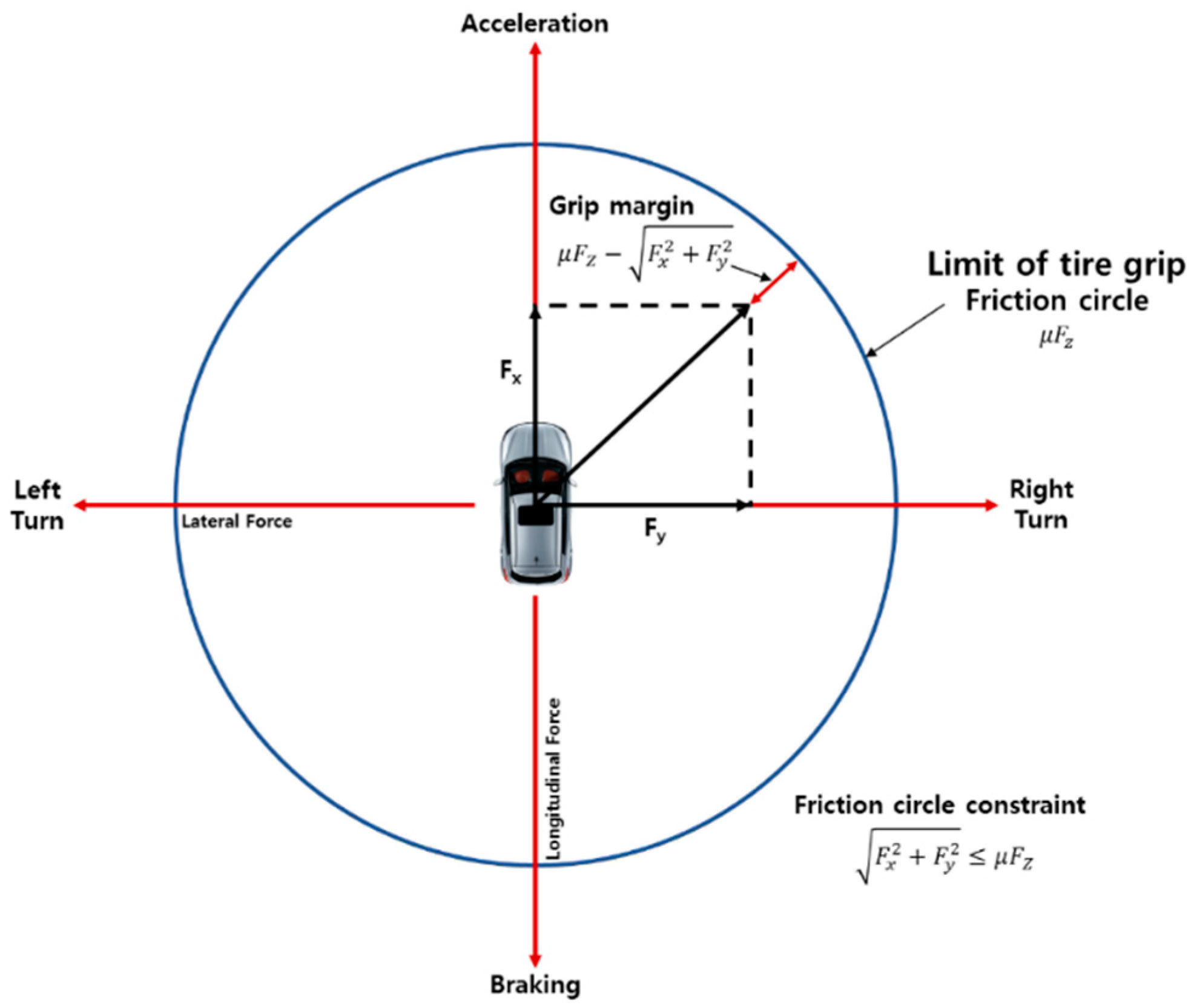
The target vehicle is driven through four in-wheel motors. At this time, the driving/braking torque is determined by the driver’s accelerator pedal or brake pedal. However, if the torque is controlled by merely reflecting the will of the driver, the vehicle may fall into an unstable state. Therefore, in this study, the stability of the vehicle is secured through slip control, yaw rate control.

2.1. Slip Control

Figure 1 shows Coulomb’s friction circle [17]. The friction circle indicates that the vector sum of the longitudinal force and lateral force of the tire is less than or equal to the product of the normal force and the friction coefficient of the road surface [18,19,20].

$$\mu F_z\ge \sqrt{F_x^2+F_y^2}$$

(1)

where μ is the coefficient of friction, F_z is the normal force of the tire, F_x is the longitudinal force of the tire, and F_y is the lateral force of the tire. In order for the vehicle to perform stable driving, the driving and braking forces should be kept not to exceed the friction circle, which is expressed as follows:

$$F_{x\_\mathit{max}}=\sqrt{{(\mu F_z)}^2-F_y^2}$$

(2)

F_{x_max} denotes the maximum drive and braking force determined by the friction circle. In other words, the driving force limit can be obtained when the road friction coefficient, the normal force and the lateral force are known. However, the normal force cannot be measured from the sensor during the driving in real time, so Equation (3) is needed to get normal force values.

$$\begin{gathered} F_{zfl}=\frac{1}{2}\frac{L_r}{L}mg-{\rho }_f{a}_{y}m\frac{h_g}{t_f}-a_{\chi }m\frac{h_g}{L} \\ {F}_{zfr}=\frac{1}{2}\frac{L_r}{L}mg+{\rho }_f{a}_{y}m\frac{h_g}{t_f}-a_{x}m\frac{h_g}{L} \\ {F}_{zrl}=\frac{1}{2}\frac{L_f}{L}mg-{\rho }_r{a}_{y}m\frac{h_g}{t_r}+a_{x}m\frac{h_g}{L} \\ {F}_{zrr}=\frac{1}{2}\frac{L_f}{L}mg+{\rho }_r{a}_{y}m\frac{h_g}{t_r}+a_{x}m\frac{h_g}{L} \end{gathered}$$

(3)

where $F_{zfl}$, $F_{zfr},F_{zrl}$ and $F_{zrr}$ are the normal force of each tire. g is the gravitational acceleration. Front and rear roll stiffness distributions are defined as ${\rho }_f$ and ${\rho }_r$. $h_g$ means the height of the center of gravity, and the accelerations of longitudinal direction and lateral direction are a_x and a_y. $t_f$ and $t_r$ are the front and rear tread lengths of the vehicle. L is the wheelbase, L_f and L_r are the distance from the center of gravity to the front wheel and rear wheel.

Lateral acceleration is generated in the vehicle when turning, and the lateral force is generated in the tire in order to cope with lateral acceleration. In this paper, the Dugoff tire model is used to formulate the nonlinear characteristics of the lateral forces in the tire [20,21].

The Dugoff tire model expresses the lateral force of a nonlinear tire as a function of the slip angle (α), the longitudinal slip rate (λ_x), the cornering stiffness (C_α) and the tire longitudinal stiffness (C_λ) that occur in each tire. Since the cornering stiffness and longitudinal stiffness of an actual tire are very different, the Dugoff tire model enables more precise tire behavior analysis compared with a linearly-expressed formula proportional to the cornering stiffness. In addition, in the actual Dugoff tire model, it is assumed that the vertical force of the tire is constant, but in this paper, the change is reflected including the previously estimated vertical force. However, the cornering stiffness is assumed to be a constant.

$$\begin{array}{l}{\alpha }_f={\delta }_f-\frac{V_y+L_f\gamma }{V_x}\\ {\alpha }_r=-\frac{V_y-L_r\gamma }{V_x}\end{array}$$

(4)

$$\begin{array}{l}{\lambda }_x=\frac{V_x-r{\omega }_w}{V_x}(duringbraking)\\ {\lambda }_x=\frac{r{\omega }_w-V_x}{r{\omega }_w}(duringacceleration)\end{array}$$

(5)

where δ_f is the front wheel steering angle, γ is the yawrate of the vehicle, r and ω_w are the effective radius of rotation and angular velocity of the tire respectively. Cornering stiffness and tire longitudinal stiffness are C_α and C_λ. The tire lateral force using the Dugoff tire model is expressed as follows:

$$F_y=C_{\alpha }\frac{\tan (\alpha )}{1+{\lambda }_x}f(\kappa )$$

(6)

where $f(\kappa )$ and the variable κ are obtained as follows:

$$\begin{gathered} f(\kappa )=\{\begin{array}{cc}(2-\kappa )\kappa & (\kappa <1)\\ 1& (\kappa \ge 1)\end{array} \\ \kappa =\frac{\mu F_z(1+{\lambda }_x)}{2{[{(C_{\lambda }{\lambda }_x)}^2+{(C_{\alpha }\tan (\alpha ))}^2]}^{1/2}} \end{gathered}$$

(7)

Finally, the lateral forces generated on each tire using the Dugoff tire model are defined as follows:

$$\begin{array}{l}{F}_{yfl}=C_{af}\frac{\tan ({\alpha }_{fl})}{1+{\lambda }_{xfl}}f({\kappa }_{fl})\\ F_{yfr}=C_{af}\frac{\tan ({\alpha }_{fr})}{1+{\lambda }_{xfr}}f({\kappa }_{fr})\\ F_{yrl}=C_{ar}\frac{\tan ({\alpha }_{rl})}{1+{\lambda }_{xrl}}f({\kappa }_{rl})\\ F_{yrr}=C_{ar}\frac{\tan ({\alpha }_{rr})}{1+{\lambda }_{xrr}}f({\kappa }_{rr})\end{array}$$

(8)

A simulation was performed to verify the lateral forces estimated in this way. The simulation was performed using CarSim 8.0 and MATLAB/Simulink 2012a. Simulation parameters such as vehicle weight, wheelbase and tread lengths used for simulation were attached as an appendix, and parameters of vehicle velocity and acceleration were used assuming CarSim’s data as sensor signals. Conditions of the simulation were set to a cruise driving situation after acceleration to 50 km/h with the steering angle fixed at 100°. Figure 2 shows the simulation results. FL, FR, RL and RR mean front left wheel, front right wheel, rear left wheel and rear right wheel respectively. The simulation on the left side is the result of assuming the normal force of the Dugoff tire model as the normal force on each wheel when the vehicle is at a stop. The simulation on the right side is the result of using normal force predicted by Equation (3). A moving average filter was applied to secure the reliability of the predicted normal force value. Despite the fact that the vehicle reached normal turning status with an estimator based on fixed normal force, the error of maximum lateral force was about 800 N, showing an accuracy of about 79%. On the contrary, when the vehicle reached normal turning state with an estimator based on the predicted normal force, the error of maximum lateral force was about 140 N, showing an accuracy of about 95.3%. Especially, outer wheels that can a have direct effect on the driving stability of the vehicle while turning were found to have high accuracy in an excessive turning situation.

Using the normal force and the lateral force obtained above, the limit driving torque can be obtained as follows:

$$\begin{array}{l}{T}_{\mathit{Slip}\_\mathit{limit}\_\mathit{fl}}=r{F}_{x\_\mathit{max}\_fl}=r\sqrt{{(\mu F_{zfl})}^2-F_{yfl}^2}\\ T_{\mathit{Slip}\_\mathit{limit}\_\mathit{fr}}=r{F}_{x\_\mathit{max}\_fr}=r\sqrt{{(\mu F_{zfr})}^2-F_{yfr}^2}\\ T_{\mathit{Slip}\_\mathit{limit}\_\mathit{rl}}=r{F}_{x\_\mathit{max}\_rl}=r\sqrt{{(\mu F_{zrl})}^2-F_{yrl}^2}\\ T_{\mathit{Slip}\_\mathit{limit}\_\mathit{rr}}=r{F}_{x\_\mathit{max}\_rr}=r\sqrt{{(\mu F_{zrr})}^2-F_{yrr}^2}\end{array}$$

(9)

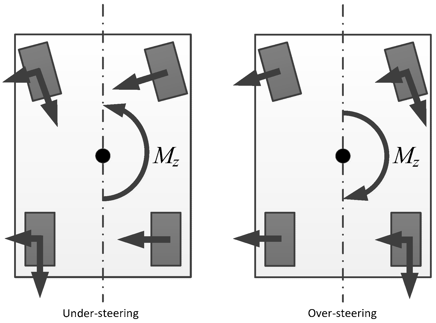
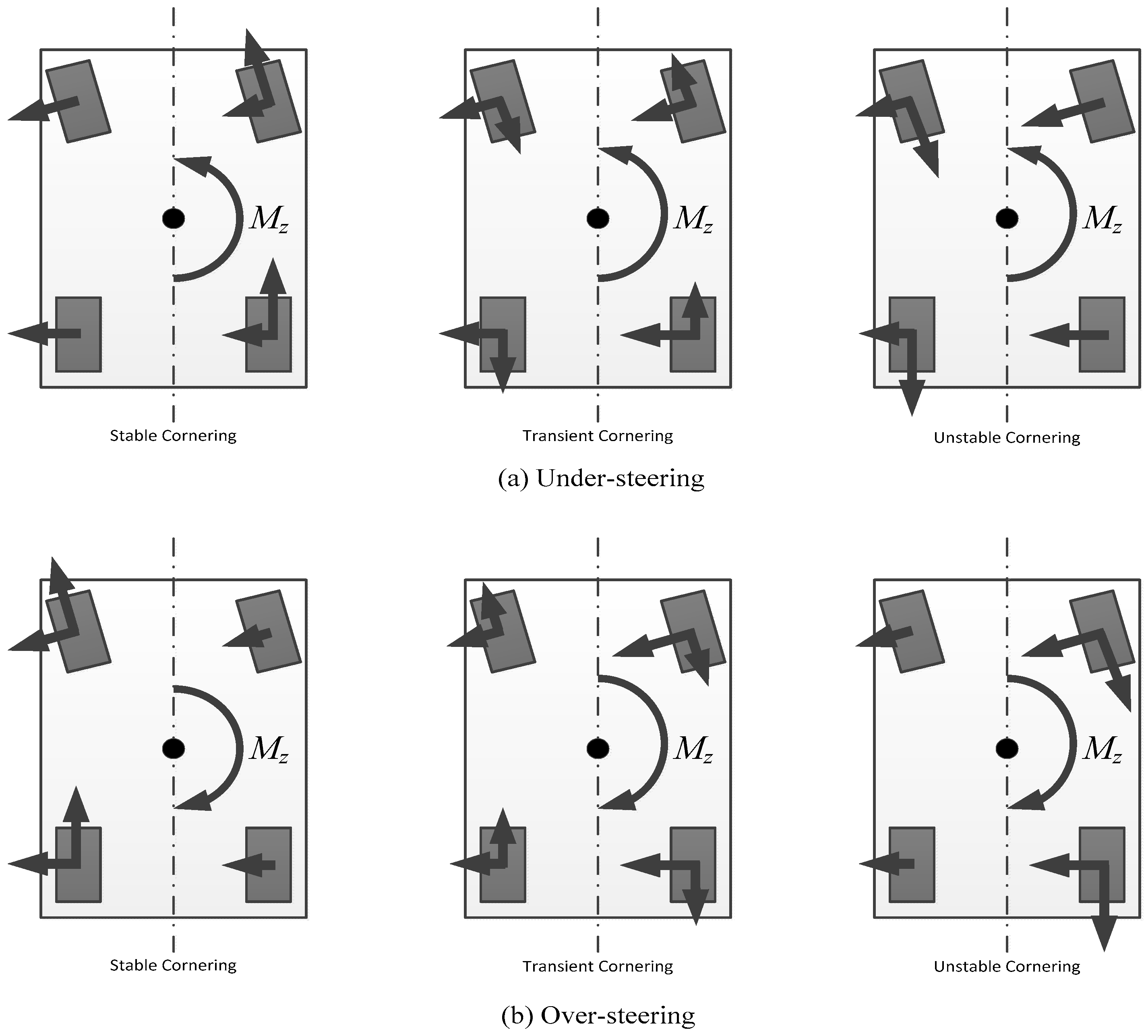
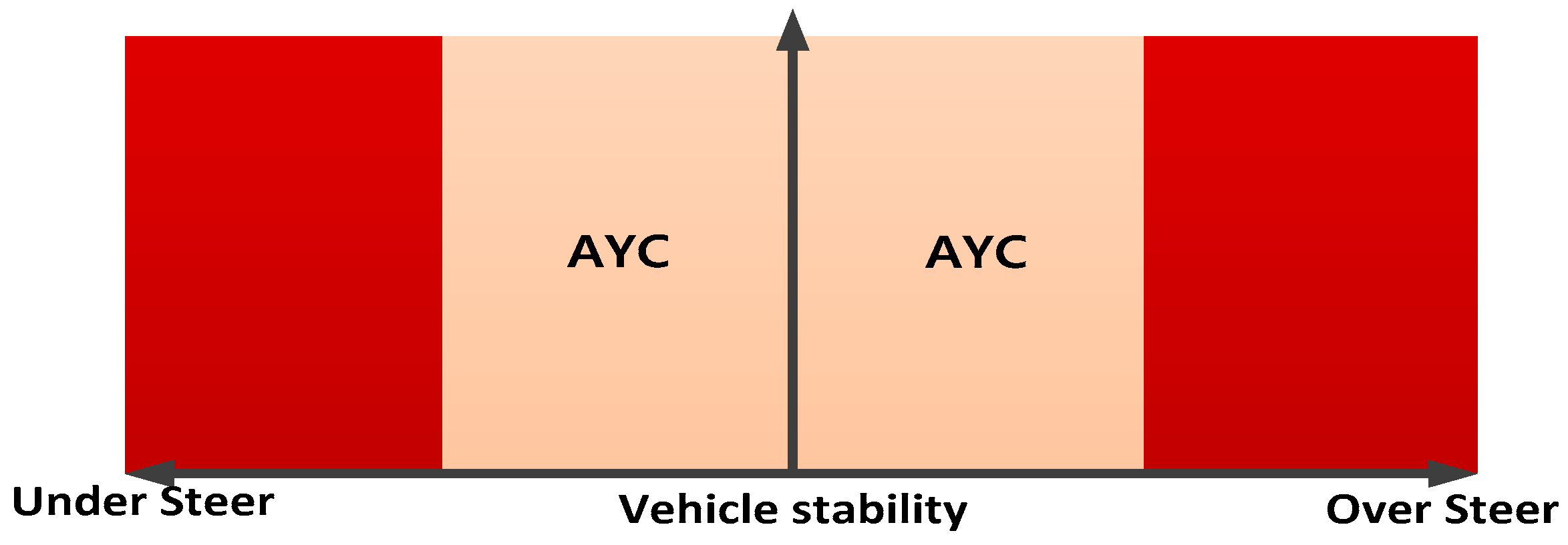
2.2. Active Yawrate Control Considering Driving Efficiency

The bicycle model has been used for the design of direct yaw moment control (DYC) in many previous researches. The desired yaw rate can be easily and exactly calculated to guarantee yaw stability based on the bicycle model through the driver’s steering intention. As shown in Figure 3, the bicycle model indicates vehicle lateral dynamics in an assumption that wheels are located at the vehicle center line.

The dynamic equations of the bicycle model in terms of force balance and moment balance are expressed as follows [22]:

$$\begin{array}{cc}\hfill m{V}_x(\dot{\beta }+\gamma )& =C_f\left({\delta }_f-\beta -\frac{L_f\gamma }{v}\right)+C_r\left(-\beta +\frac{L_r\gamma }{v}\right)\hfill \\ \hfill {}_z\dot{\gamma }& =L_f{C}_f\left({\delta }_f-\beta -\frac{L_f\gamma }{V_x}\right)-L_r{C}_r\left(-\beta +\frac{L_r\gamma }{V_x}\right)+M_z\hfill \end{array}$$

(10)

where β is the body side slip angle, γ is the yaw rate, m is the vehicle mass, I_z is the vehicle yaw moment of inertia, V_x is the vehicle longitudinal velocity, and M_z is the correction yaw moment. L_f and L_r are the CG-front and CG-rear axle distances, F_yf and F_yr are the lateral tire forces of the front and rear axle, respectively. C_f and C_r are the front and rear wheel cornering stiffness and δ_f is the steering angle. State-space expression of the bicycle model is given as follows:

$$\left[\begin{array}{c}\dot{\beta }\\ \dot{\gamma }\end{array}\right]=\left[\begin{array}{cc}\frac{-C_f-C_r}{m{V}_x}& \frac{-m{V}_x{}^2-L_f{C}_f+L_r{C}_r}{m{V}_x{}^2}\\ \frac{-L_f{C}_f+L_r{C}_r}{I_z}& \frac{-L_f{}^2{C}_f-L_r{}^2{C}_r}{V_x{I}_z}\end{array}\right]\left[\begin{array}{c}\beta \\ \gamma \end{array}\right]+\left[\begin{array}{cc}\frac{C_f}{m{V}_x}& 0\\ \frac{L_f{C}_f}{I_z}& \frac{1}{I_z}\end{array}\right]\left[\begin{array}{c}{\delta }_f\\ M_z\end{array}\right]$$

(11)

where L is the wheelbase. The desired yawrate can be expressed as a function of the steering angle δ_f and the vehicle longitudinal velocity V_x. It is represented as follows:

$${\gamma }_d=\frac{V_x}{L+\frac{m{V}_x{}^2(L_r{C}_r-L_f{C}_f)}{2C_f{C}_{r}L}}{\delta }_f$$

(12)

The desired yaw moment to follow the desired yaw rate is defined as follows:

$$M_z=I_z{\dot{\gamma }}_d+(C_f{L}_f-C_r{L}_r)\beta +\frac{C_f{L}_f^2+C_r{L}_r^2}{V_x}\gamma -C_f{L}_f\delta -\eta I_z(\gamma -{\gamma }_d)$$

(13)

where η is a positive constant. In the lower controller, the control input in (13) consists of the individual tire forces generated by the in-wheel motor system. The correction yaw moment is obtained as follows:

$$M_z=t_f\cos ({\delta }_f)(F_{xfr}-F_{xfl})+L_f\sin ({\delta }_f)(F_{xfr}+F_{xfl})+t_f\sin ({\delta }_f)(F_{yfl}-F_{yfr})+t_r(F_{xrr}-F_{xrl})$$

(14)

Assuming that the steering angle is small, sin(δ) is assumed to be zero. Equation (14) is rewritten as follows:

$$M_z=t_f\cos ({\delta }_f)(F_{xfr}-F_{xfl})+t_r(F_{xrr}-F_{xrl})$$

(15)

Since the VDC of an internal combustion engine vehicle or ordinary electric vehicle is difficult to control the driving force independently, the correction moment for over steering or under steering during a left turn is generated as shown in Figure 4. Such a correction moment can improve the driving stability of a vehicle, but it can decrease the velocity of the vehicle as well. Velocity decrease not only makes the driver feel odd while driving but also causes additional driving force, which leads to the low driving efficiency of the vehicle.

To solve this problem, cornering situations were classified and a driving force distribution strategy was proposed as shown in Figure 5. Cornering situations are largely divided into three types, namely stable cornering, transient cornering and unstable cornering. Stable cornering is a driving situation in which the velocity of the vehicle is relatively slow and the desired yaw rate is low, so the driving torque of the motor is not expected to have a critical impact on driving stability. Thus, the correction yaw moment is generated through driving torque. Excessive cornering is a domain in which vehicle velocity and desired yaw rate have intermediate values. Since excessive driving torque can make the vehicle unstable, correction yaw moment is generated using both the driving force and braking force. Lastly, unstable cornering is a situation of high velocity or high desired yaw rate where the driving torque can greatly affect the driving stability. Correction yaw moment is generated only using braking force. To satisfy such rules, a controller needs to be comprised so that three yaw moment distribution strategies intervene according to the situation. However, there is a problem that excessive mode conversion occurs when the vehicle is operated around the mode conversion point. A Fuzzy controller was used to prevent excessive switching errors while fulfilling such a purpose. The fuzzy logic has been proposed to solve the problems of various logic which judged only the existing true and false, and it can output various values between 0 and 1. It is employed to handle the concept of partial truth, where the truth value may range between completely true and completely false [23]. Composition of the fuzzy controller is as presented in

Table 1. Cornering stability Index.

Fuzzy Controller Input Membership Function	Fuzzy Controller Rule Base
Fuzzy Controller Output Membership Function	Fuzzy Control Surface

. The input membership function of the fuzzy controller includes the velocity of the vehicle and desired yaw rate. Output membership function outputs the cornering stability index (σ) with a value of 0~2. Cornering stability index indicates a stable cornering situation as it gets closer to 0 and an unstable cornering situation as it gets closer to 2. Final AYC (Active Yawrate Control) torque output is defined as Equation (16). The operating region of AYC is shown in Figure 6.

$$\begin{array}{l}{T}_{fl\_AYC}=\begin{array}{cc}{T}_{fl}(APS,BPS)\pm T_{fl\_stable}(1-\sigma )\pm T_{fl\_trans}(\sigma )\hfill & \hfill (\sigma \le 1)\\ T_{fl}(APS,BPS)\pm T_{fl\_trans}(2-\sigma )\pm T_{fl\_unstable}(\sigma -1)\hfill & \hfill (1<\sigma \le 2)\end{array}\\ T_{fr\_AYC}=\begin{array}{cc}{T}_{fr}(APS,BPS)\pm T_{fr\_stable}(1-\sigma )\pm T_{fr\_trans}(\sigma )\hfill & \hfill (\sigma \le 1)\\ T_{fr}(APS,BPS)\pm T_{fr\_trans}(2-\sigma )\pm T_{fr\_unstable}(\sigma -1)\hfill & \hfill (1<\sigma \le 2)\end{array}\\ T_{rl\_AYC}=\begin{array}{cc}{T}_{rl}(APS,BPS)\pm T_{rl\_stable}(1-\sigma )\pm T_{rl\_trans}(\sigma )\hfill & \hfill (\sigma \le 1)\\ T_{rl}(APS,BPS)\pm T_{rl\_trans}(2-\sigma )\pm T_{rl\_unstable}(\sigma -1)\hfill & \hfill (1<\sigma \le 2)\end{array}\\ T_{rr\_AYC}=\begin{array}{cc}{T}_{rr}(APS,BPS)\pm T_{rr\_stable}(1-\sigma )\pm T_{rr\_trans}(\sigma )\hfill & \hfill (\sigma \le 1)\\ T_{rr}(APS,BPS)\pm T_{rr\_trans}(2-\sigma )\pm T_{rr\_unstable}(\sigma -1)\hfill & \hfill (1<\sigma \le 2)\end{array}\end{array}$$

(16)

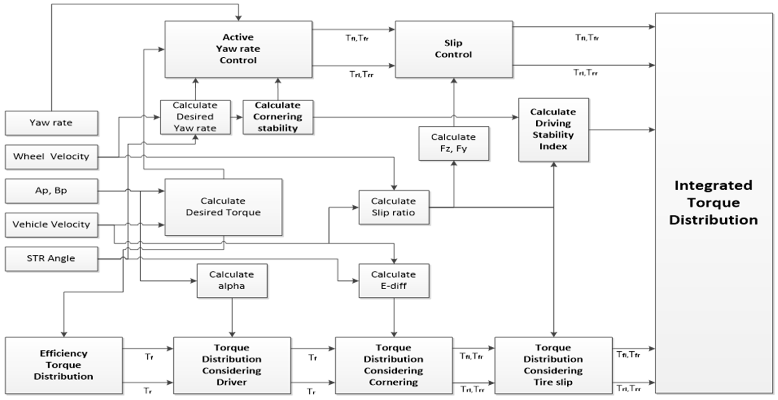
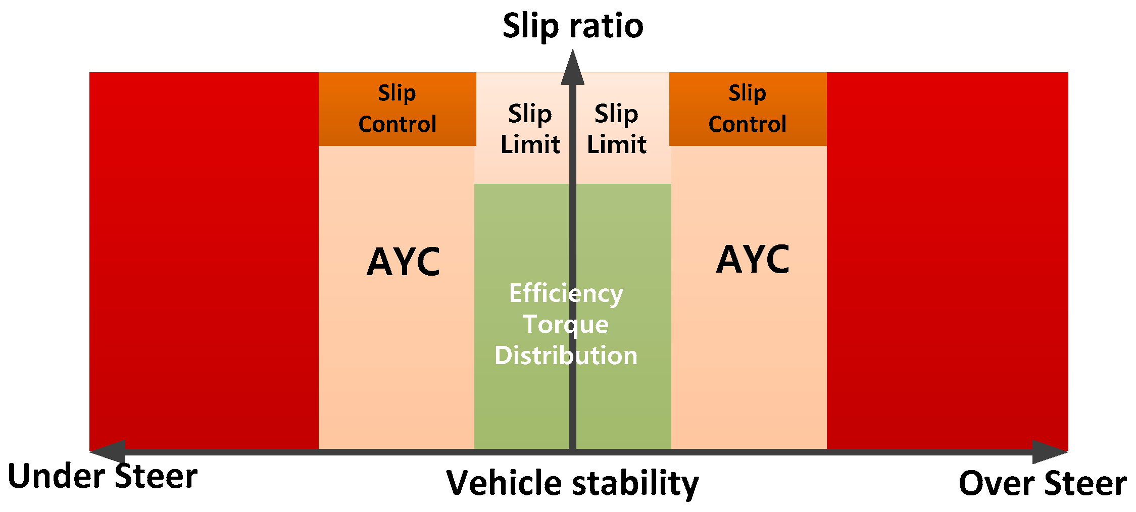
2.3. Integrated Driving Torque Distribution Strategy Considering Driving Efficiency and Stability

When a vehicle accelerates or climbs a hill while driving, it requires a large amount of driving force. However, the desire of the driver can be followed without using the maximum torque of the motor in case of cruise drive or downhill drive. Generating same driving torque on four wheels makes it difficult to drive the motor in the efficient region. As a solution to this problem, a driving torque distribution strategy that appropriately distributes the driving force and regenerative braking force of the front and rear wheels according to the situation to improve the efficiency of the vehicle was proposed as described in previous paper [24]. However, since the developed distribution strategy is a strategy that considers driving efficiency in a stable situation, there is a problem of reducing driving stability of the vehicle in a rapid cornering situation or low-friction road situation. The following driving stability index (ψ) was proposed to solve this problem.

$$\psi =\frac{1}{\tilde{\lambda }}(\lambda )(\lambda >0.1)+\frac{1}{\tilde{\dot{\lambda }}}(\dot{\lambda })(\lambda >0.1)+\frac{1}{\tilde{\sigma }}(\sigma )+\frac{1}{\tilde{\dot{\sigma }}}(\dot{\sigma })$$

(17)

where $\lambda$ is the slip rate, $\tilde{\lambda }$ is the slip rate limit, $\dot{\lambda }$ is the differential value of slip rate, $\tilde{\dot{\lambda }}$ is the differential value limit of slip rate, $\sigma$ is the cornering stability index, $\tilde{\sigma }$ is the cornering stability index limit, $\dot{\sigma }$ is the differential value of cornering stability index, and $\tilde{\dot{\sigma }}$ is the differential value limit of the slip rate. Each term represents the ratio of the current value to the limit value that determines driving stability. For instance, if the slip rate limit is 0.2 and the current slip rate is 0.15, the stability index for slip rate of the vehicle is 0.75. The stability index is calculated for four variables, and the sum becomes the driving stability index of the vehicle. The inequality equation that constitutes the term that determines the stability of the slip rate was added to decide the stability of the slip rate only in the area where the slip rate becomes larger than 0.1 by considering the area with a slip rate smaller than 0.1 as a stable area. If one of four variables that constitute Equation (17) has a value larger than 1, the vehicle is considered to be in an unstable state and is controlled only using the torque for improving driving stability. However, if the value is between 0 and 1, the driving stability evaluation index is used as a weight factor to determine the intervention rate of the efficiency controller and driving stability controller. The final torque values determined are expressed by the equations as follows:

$$\begin{array}{l}{T}_{fl\_final}=T_{fl\_STC}(\psi )\pm T_{fl\_Eff}(1-\psi )\\ T_{fr\_final}=T_{fr\_STC}(\psi )\pm T_{fr\_Eff}(1-\psi )\\ T_{rl\_final}=T_{rl\_STC}(\psi )\pm T_{rl\_Eff}(1-\psi )\\ T_{rr\_final}=T_{rr\_STC}(\psi )\pm T_{rr\_Eff}(1-\psi )\end{array}$$

(18)

where T_STC is torque determined to improve the driving stability of the vehicle, and T_Eff is the torque value determined to increase the efficiency of the vehicle. The vehicle stability index has values from 0 to 1, and the values close to 1 equate to unstable values. If the vehicle stability index is 1, only the T_STC is determined to be the output torque by (1 − ψ) term, and if the evaluation index is 0, only the T_eff is configured to be an output. Sometimes the final torque may exceed the T_stc, but the simulation found that the stability of the driving was less affected. It seems that when the final torque affects the driving stability of the vehicle, only the T_stc is output as the vehicle stability index becomes 1. The final torque, thus determined, controls the driving stability and efficiency of the vehicle through four in-wheel motors.

The block diagram of the integrated torque distribution strategy is shown in Figure 7. The torque distribution strategy for increased efficiency proposed in previous papers is located at the bottom of the block diagram. The slip controller and AYC proposed in this paper are located at the top of the block diagram. Driving efficiency and driving stability of the vehicle were secured in the end by determining the intervention rate of these two torque distribution strategies using the driving stability evaluation index.

The operating region of ITD is shown in Figure 8. In the area where the vehicle is determined to be stable, the distribution strategy for increased efficiency primarily intervenes. In the area where the instability of the vehicle increases, driving stability and driving efficiency are secured using the slip controller and AYC.

3. Simulation and Experimental Results

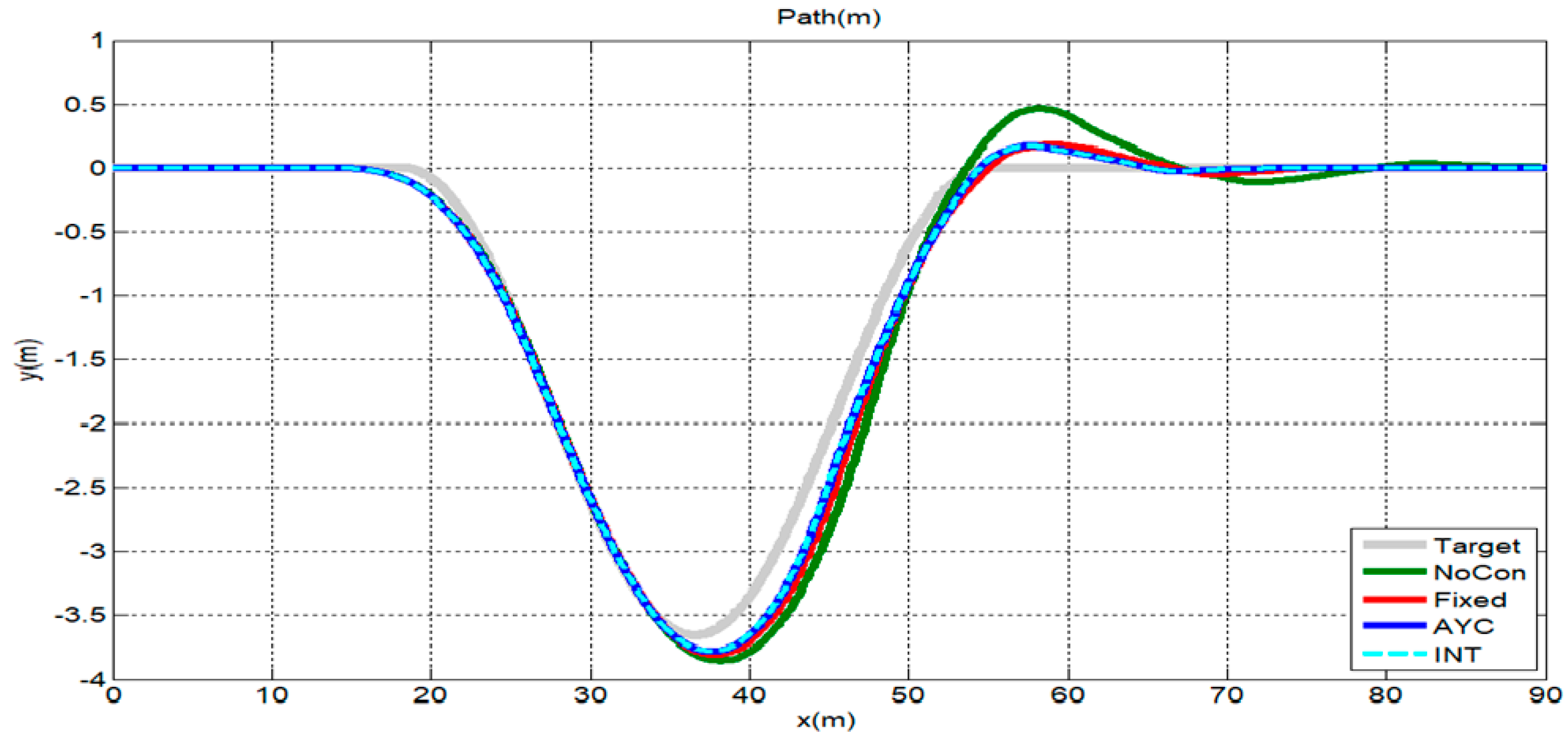
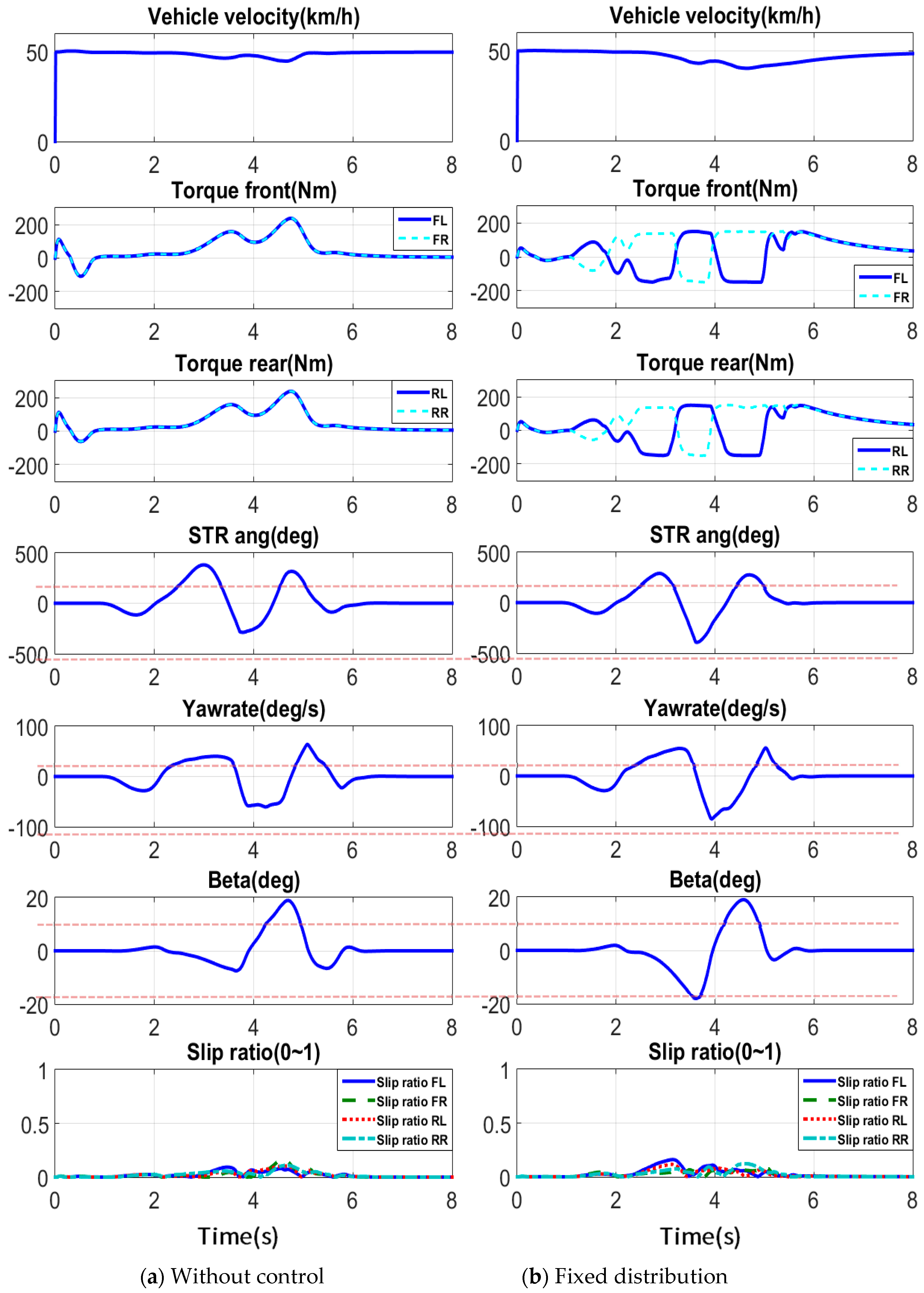
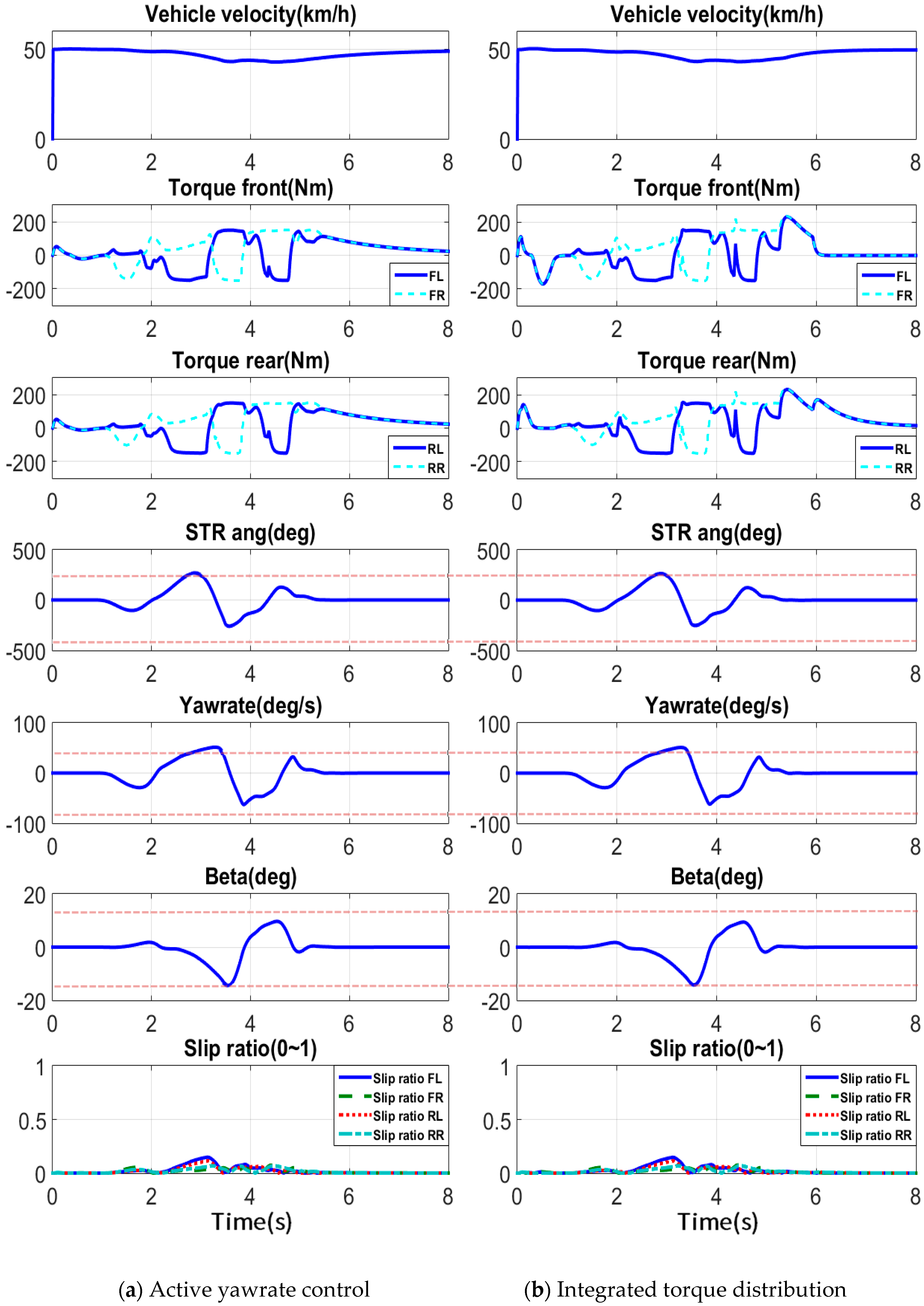
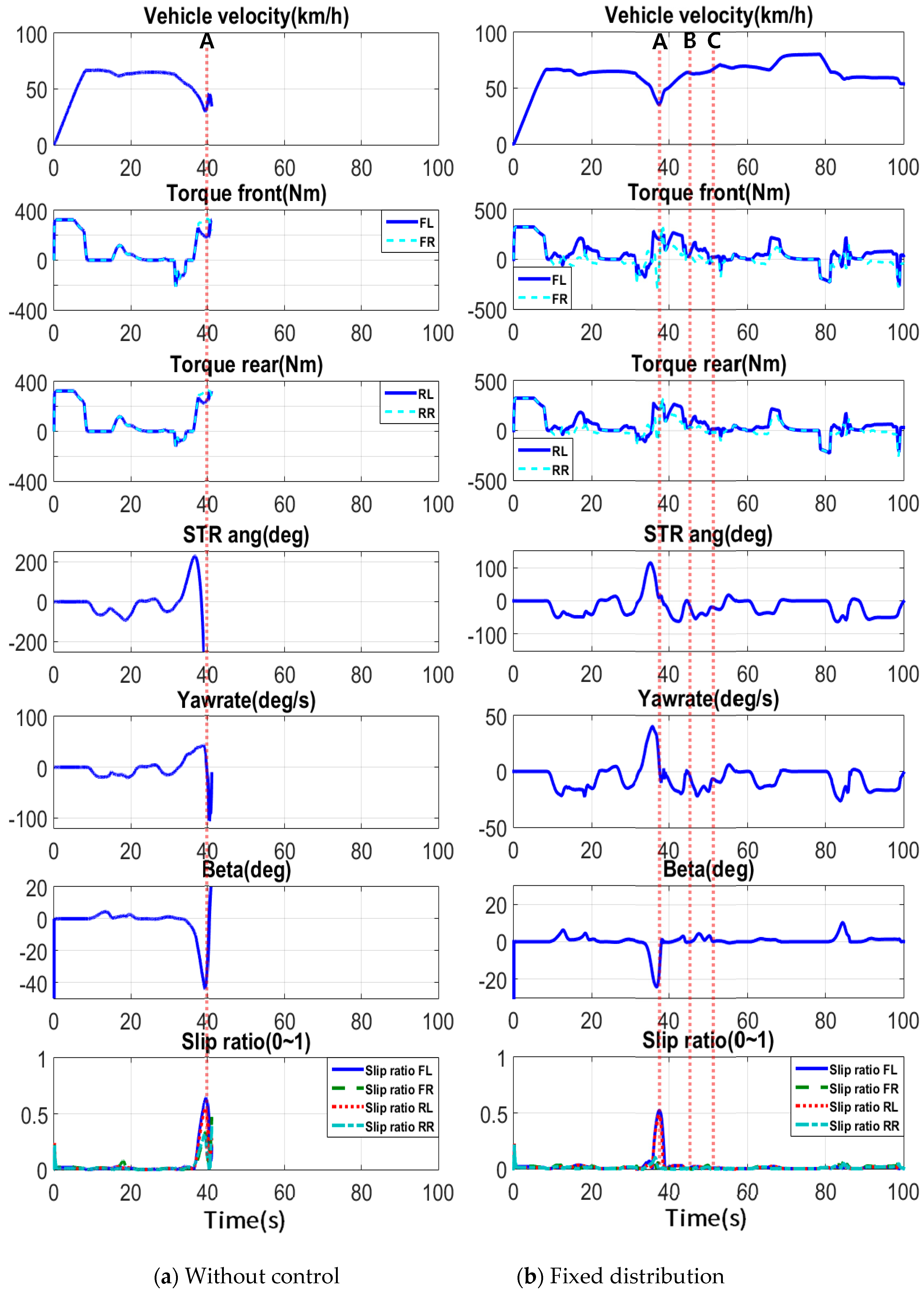
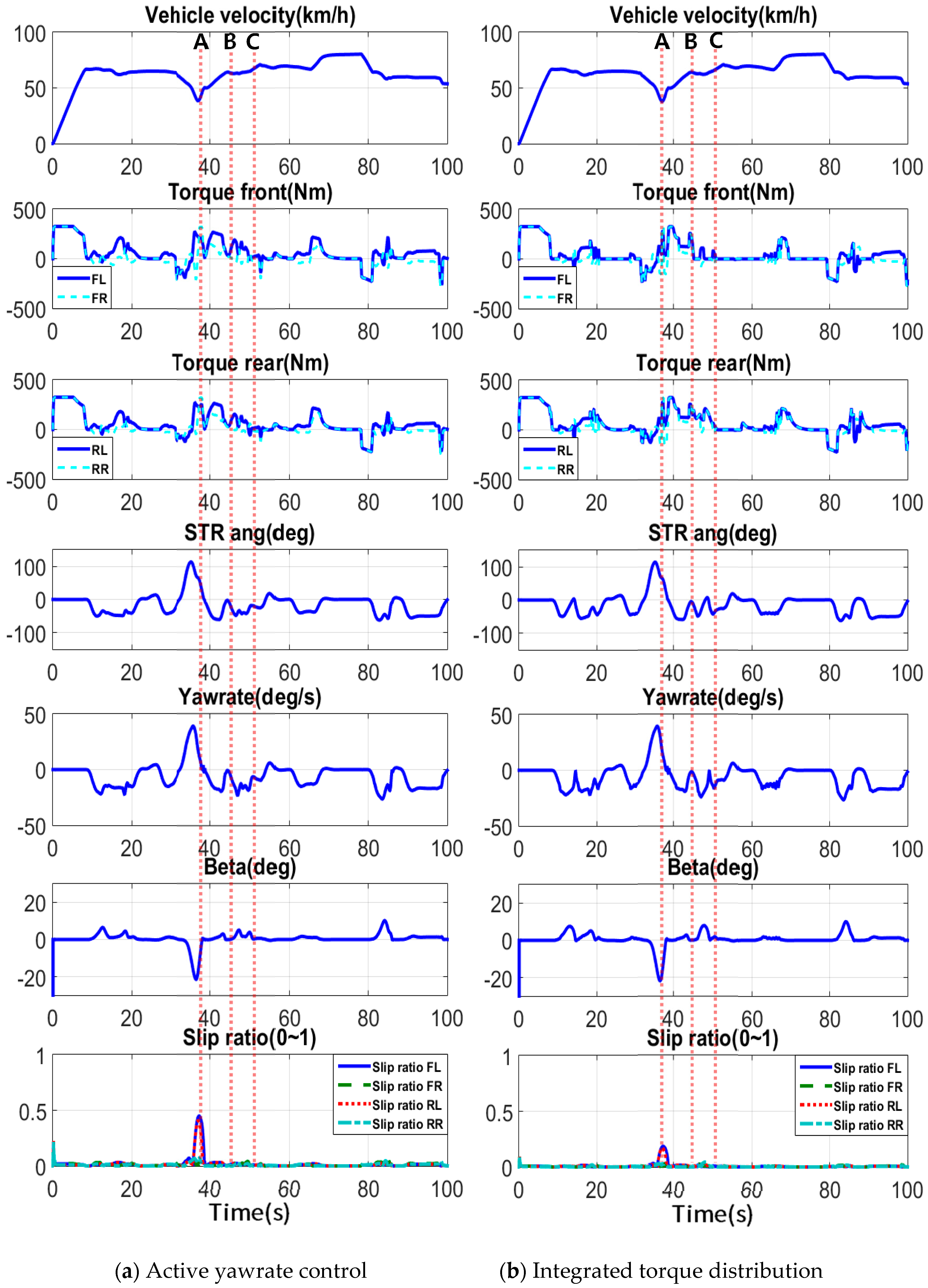
3.1. Double Lane Change Simulation

A double-lane change simulation was performed to identify the effect of the proposed torque distribution strategy on the driving stability of the vehicle. The ISO double lane change test consists of an entry and an exit lane and has a length of 12 m and a side lane with a length of 11 m. The width of the entry and side lane are dependent on the width of the vehicle; the width of the exit lane is constantly 3 m wide. The lateral offset between the entry and side lane is 1 m and the longitudinal offset is 13.5 m. For the same lateral offset, the side and exit lane have a slightly shorter longitudinal displacement of 12.5 m. The simulation was performed at a target speed of 50 km/h to verify the performance of the AYC. Driving trajectory is shown in Figure 9. The road friction condition was 0.5 of a wet road. According to the simulation results, vehicles without a torque distribution strategy showed a large over shoot of about 0.46 m, whereas vehicles applied with the torque distribution strategy showed a small over shoot of about 0.18~0.19 m. Vehicles applied with AYC have similar behavior as vehicles applied with integrated torque distribution (ITD). Since this is a low velocity situation with a high desired yaw rate, the final driving torque determined by the vehicle stability index (ψ) places a greater priority on the driving stability control than the efficiency control.

Detailed simulation results are shown in Figure 10 and Figure 11. The x-axis of each graph represents the time, and the y-axis represents the data and units of each graph title. FL, FR, RL and RR mean front left wheel, front right wheel, rear left wheel and rear right wheel respectively. The trend line for comparison was based on vehicles without a torque distribution strategy. Based on the comparison of motor torque, vehicles applied with AYC and ITD showed relatively similar tendencies, but torque output differs between 0~1 seconds section and 5~6 seconds section. As this section is a section in which the vehicle drives straight, the torque distribution strategy intervenes to improve driving efficiency. The steering wheel input is largest in vehicles without a torque distribution strategy, and cases applied with AYC and ITD show similar values. Based on the yaw rate of 1~4 seconds section, vehicles without a torque distribution strategy have a low yaw rate despite having larger steering input compared to other vehicles. This is probably caused by correction yaw moment according to the application of the torque distribution strategy. However, vehicles without a torque distribution strategy have the highest yaw rate in 4~5 seconds section. This section is the 55~65 m region of driving trajectory shown in Figure 9. Excessive steering value results from increasing the deviation from the driving path. Vehicles applied with AYC and vehicles applied with ITD have similarly small values of side slip angle, which is used to determine the driving stability of a vehicle while cornering. This is probably because if the vehicle without ITD is not able to follow the driver’s desired path, the driver enters a larger steering angle. On the other hand, if the vehicle to which the ITD is applied does not follow the driver’s desired path, ITD will assist with the motor driving torque, so the driver will maintain the small steering input. Thus, if the driver maintains a small steering input, the probability that the vehicle will go into an unstable state is reduced.

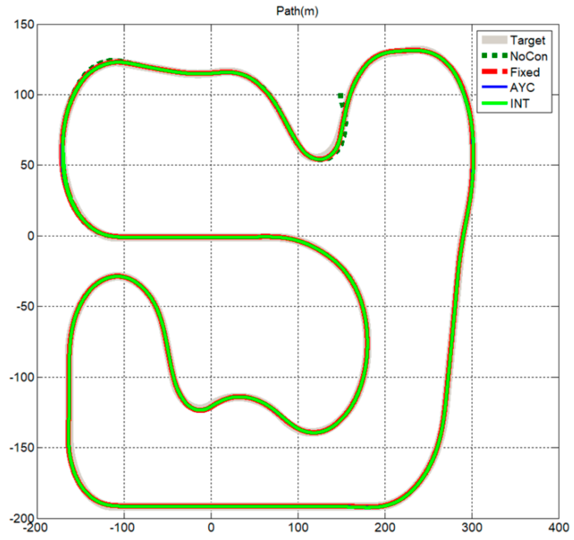
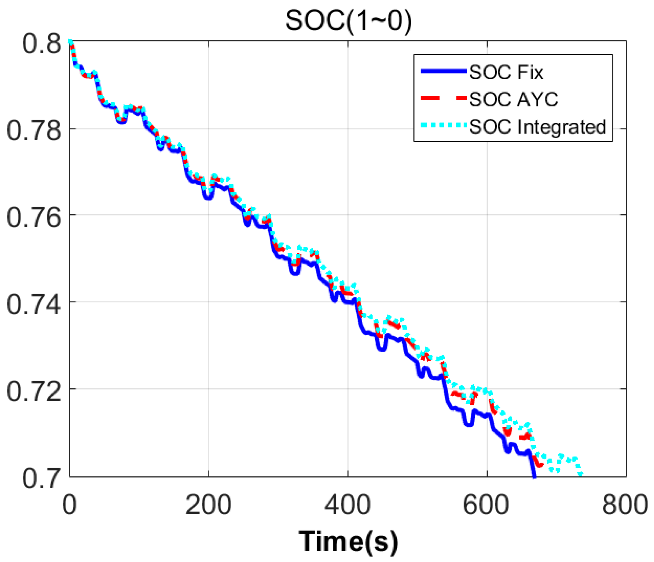
3.2. Complex Driving Road Simulation

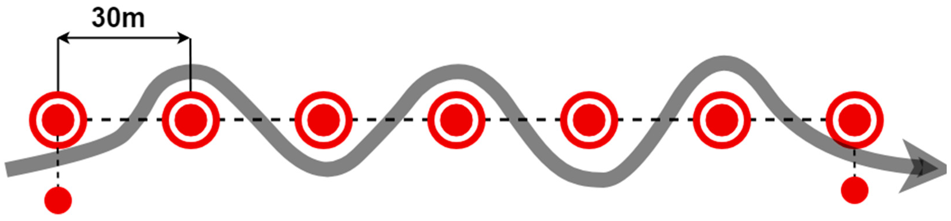
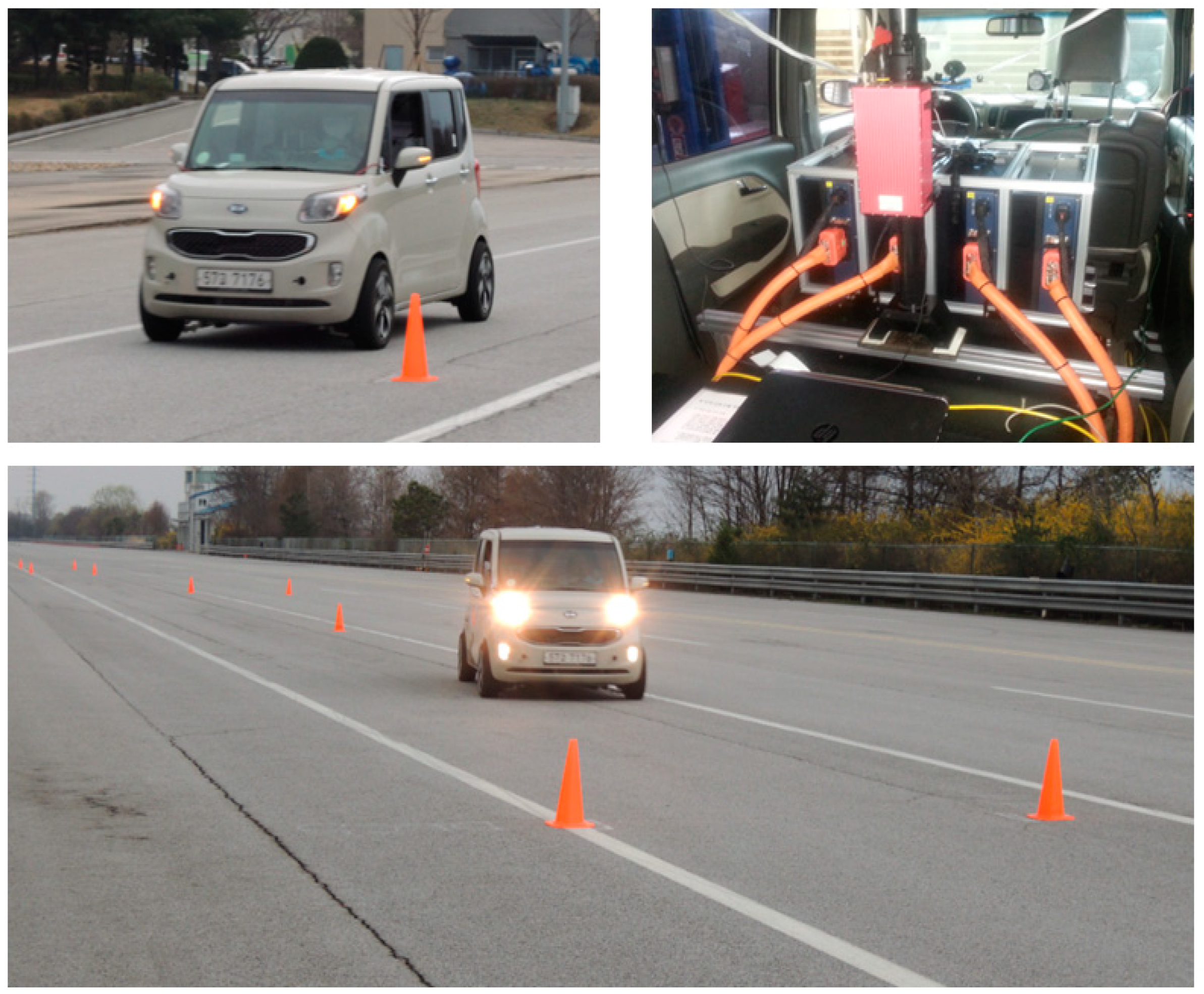
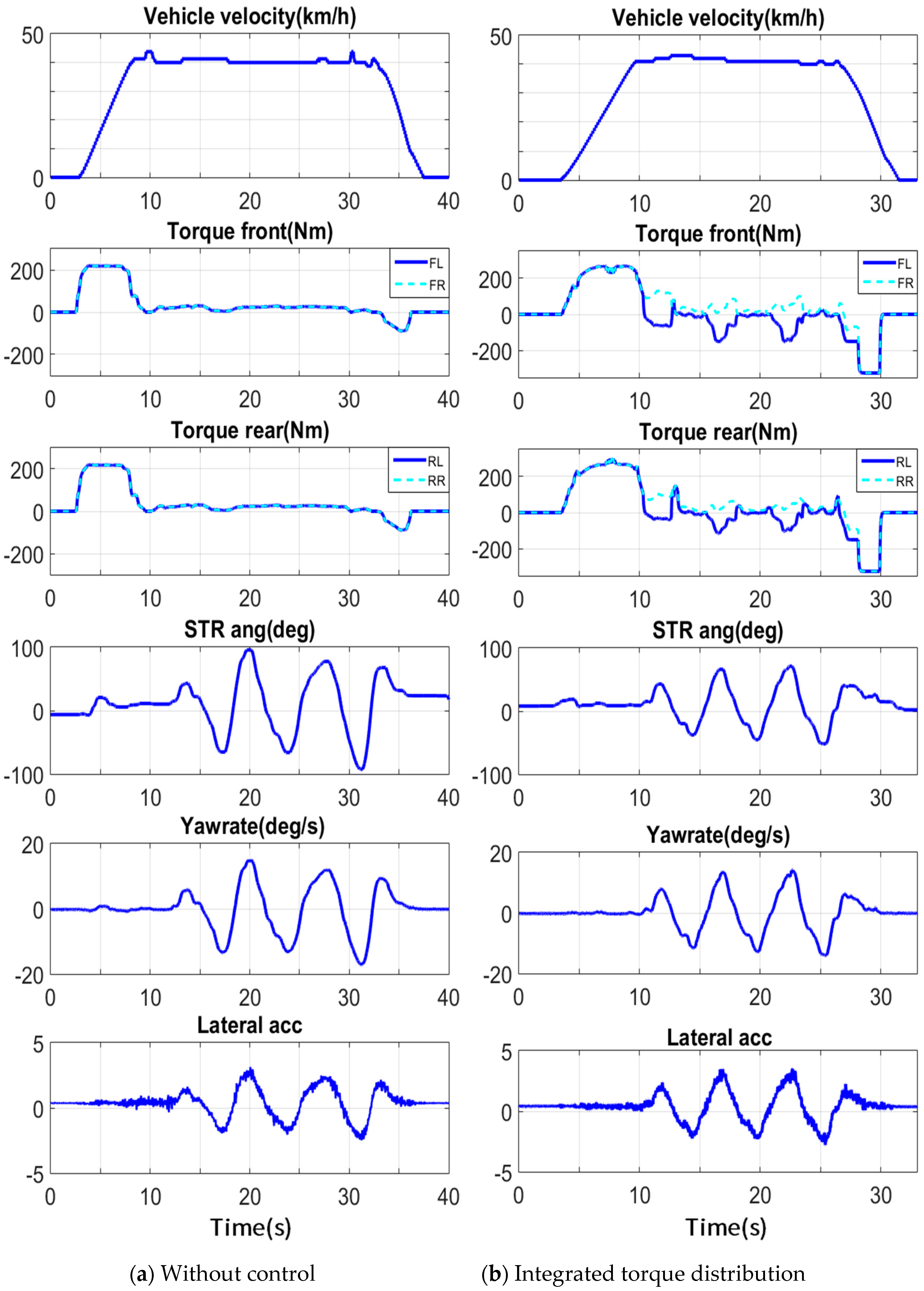
A simulation was carried out to verify the overall performance of the proposed torque distribution strategy. Target driving path for the simulation and the result of driving according to the distribution strategy are shown in Figure 12. Road condition was configured as 0.5 of a wet road for driving stability assessment.

The simulation was performed on a case without a torque distribution strategy, a case with left and right fixing torque distribution, a case applied with active yaw rate control, and a case applied with integrated torque distribution. Comparing the results of driving trajectory, vehicles without a torque distribution strategy cannot follow the target driving path in the expanded region and roll over occurs. On the contrary, vehicles applied with the three torque distribution strategies show similar path following.

Figure 13 and Figure 14 show detailed simulation results according to the application of each distribution strategy. The x-axis of each graph represents time, and the y-axis represents the data and units of each graph title. FL, FR, RL and RR mean front left wheel, front right wheel, rear left wheel and rear right wheel respectively. The results for points A, B and C were analyzed to compare the driving performance according to the distribution strategy. First, vehicles without the distribution strategy generate mostly identical torque in all motors despite a large amount of cornering at point A. Vehicles were found to deviate from the driving path due to a rapid increase of the yaw rate, side slip angle and slip ratio. The case applied with the left and right fixing torque distribution strategy and the case applied with AYC were found to maintain similar driving stability. However, the case applied with integrated torque distribution shows the reduced driving torque of the motor and maintains the slip ratio in a stable region compared to other distribution strategies because the slip controller intervenes at point A. However, it has a larger yaw rate and side slip angle compared to the other distribution strategies in section B-C. This is probably because the final driving torque determined by the vehicle stability index (ψ) places a greater priority on efficiency control. SOC (State of Charge) based on repeated driving of the driving path in Figure 12, intended to quantitatively compare driving efficiency according to the application of each distribution strategy, is shown in Figure 15. Driving distance based on SOC is shown in

Table 2. Simulation results of efficiency.

Performance Index	Fixed Distribution	Active Yawrate Control	Integrated Torque Distribution
Driving Distance	11.89 km	12.35 km	13.19 km
Rate of Increment	-	3.87%	10.93%

. The range of SOC is 0.8~0.7, and the driving distance from the use of 0.1 SOC was compared. The results for vehicles without a torque distribution strategy are not included because they could not be driven due to overturn. Looking at Table 2, the case applied with AYC showed total driving distance increased by about 3.87% compared to the case applied with the left and right fixing torque distribution strategy. Total driving distance was increased by about 10.93% in the case applied with integrated torque distribution. The proposed torque distribution strategy was found to increase driving efficiency while securing the driving stability of vehicles.

3.3. Vehicle Test

The actual vehicle experiment was conducted to determine the effect of the developed torque distribution strategy on the driving stability of the actual vehicle. Based on KIA automotive’s gasoline ray model, the target vehicle was equipped with an in-wheel motor for independent driving. The experimental conditions were selected as follows.

-

Test condition: Slalom course with pylon set at equal intervals of 30 m

-

Driving method: Drive as close as possible without hitting the pylon

-

Target Speed: 40 km/h

-

Measurement data: vehicle velocity, wheel steering angle, motor drive torque, yaw rate, and lateral acceleration

-

Measuring sensor: RT 3000

The velocity of the vehicle must be found accurately to apply the proposed control algorithm to the vehicle and to perform performance verification. In this paper, an experiment was conducted using the velocity signal of RT 3000 mentioned earlier. RT 3000 has an inertial navigation system that has position accuracy of about 40 cm and a velocity accuracy of 0.1 km/h. Data output rate is 100 Hz, which secures data in real time. Figure 16 shows the Slalom test course. Figure 17 shows the actual experimental scene and the sensor used during the experiment. The photograph on the top right side is the sensor attached to the vehicle.

Figure 18 shows the driving test results according to the application of ITD. The x-axis of each graph represents time, and the y-axis represents the data and units of each graph title. FL, FR, RL and RR mean front left wheel, front right wheel, rear left wheel and rear right wheel respectively. Comparing the velocity results, the two vehicles were driven while maintaining similar velocity. However, whereas the vehicle not applied with ITD maintained constant motor-driving torque, the vehicle applied with ITD showed left and right driving torques change to follow the desired yaw rate of the driver. Looking at the steering angle results, the vehicle applied with ITD showed a smaller steering angle compared to the vehicle not applied with ITD. This is probably because if the vehicle without ITD is not able to follow the driver’s desired path, the driver enters a larger steering angle. On the other hand, if the vehicle to which the ITD is applied does not follow the driver’s desired path, ITD will assist with the motor-driving torque, so the driver will maintain the small steering input.

To quantitatively compare the test results, the peak values of steering angle, yaw rate and lateral acceleration are presented in

Table 3. Peak values of slalom test results.

Signal Name	1st Peak Value	2nd Peak Value	3rd Peak Value	4th Peak Value	5th Peak Value	R.M.S Value
STR ang (deg) without ITD	−65.2	95.6	−66	77.5	−92.4	80.4
STR ang (deg) with ITD	−37.7	66.1	71.1	−45.2	−51.7	55.8
Yawrate (deg/s) without ITD	−13	15	−12.99	11.88	−17.04	14.11
Yawrate (deg/s) with ITD	−11.44	13.43	−12.73	14.16	13.97	13.2
Lateral acc without ITD	−1.95	3.13	−2.04	2.43	−2.37	2.4
Lateral acc with ITD	−2	3.49	−2.32	3.51	−2.31	2.8

. The R.M.S value of the peak value of steering angle is 80.4 for the vehicle not applied with ITD and 55.8 for the vehicle applied with ITD, which is about 30.6% smaller. Also, since the vehicle applied with ITD was able to drive with a small radius of turning, the R.M.S value of the peak value of yaw rate was also decreased by about 6.5%. On the contrary, since the vehicle applied with ITD showed a sudden change of direction compared to the vehicle not applied with ITD, the R.M.S value of the peak value of lateral acceleration was increased by about 16.7%. The vehicle was confirmed to be driven in the path wanted by the driver with relatively small steering input through the application of ITD, contributing to improved driving stability of the vehicle.

4. Conclusions

An integrated torque distribution strategy was developed to improve the stability and efficiency of the vehicle. In order to improve the stability of the low friction road surface, the vertical force and the lateral force of the vehicle were estimated and the limit driving torque was determined using the estimated force. A turning stability index comprised of vehicle velocity and desired yaw rate of the driver was proposed to examine the driving stability of the vehicle while turning. The proposed index was used to subdivide the turning situations and to propose a torque distribution strategy which can minimize deceleration of the vehicle while securing turning stability. The torque distribution strategy for increased driving stability and the torque distribution strategy for increased efficiency proposed were used to create an integrated torque distribution strategy. A vehicle stability index based on the slip rate and turning stability index was proposed to determine the overall driving stability of the vehicle, and the proposed index was used as a weight factor that determines the intervention of the control strategy for increased efficiency and the control strategy for improved driving stability.

The simulation and actual vehicle test were carried out to verify the performance of the developed ITD. Based on the short double-lane change simulation on low-friction roads, the vehicle applied with ITD showed best path tracking and the smallest reduction of velocity. Based on the results of complex road simulation, the vehicles without torque distribution strategy were overturned around sharp corners, whereas the vehicles applied with the torque distribution strategy were driven stably. In addition, the vehicle applied with ITD showed the most desirable results for driving efficiency. An actual vehicle test was performed to evaluate the performance of ITD on an actual vehicle. The test conditions were selected for slalom driving at 40 km/h. As a result of the actual vehicle test, the vehicle applied with ITD was found to be driven in the path wanted by the driver with relatively small steering input compared to the vehicle not applied with ITD. From these results, it can be confirmed that the proposed driving torque distribution strategy improves the efficiency and driving stability of the independent driving electric vehicle. This is an improvement over the various studies mentioned in the introduction, focusing only on improving the driving efficiency of the vehicle.

References

1. Hori, Y. Future Vehicle Driven by Electricity and Control-Research on Four-Wheel- Motored “UOT electric march II”. IEEE Trans. Ind. Electron. 2004, 51, 954–962. [Google Scholar] [CrossRef]
2. Nasri, A.; Hazzab, A.; Bousserhane, I.; Hadjeri, S.; Sicard, P. Fuzzy-Sliding Mode Speed Control for Two Wheels Electric Vehicle Drive. J. Electr. Eng. Technol. 2009, 4, 499–509. [Google Scholar] [CrossRef]
3. Sekour, M.; Hartani, K.; Draou, A.; Allali, A. Sensorless Fuzzy Direct Torque Control for High Performance Electric Vehicle with Four In-Wheel Motors. J. Electr. Eng. Technol. 2013, 8, 530–543. [Google Scholar] [CrossRef] [Green Version]
4. Hartani, K.; Draou, A. A New Multimachine Robust Based Anti-skid Control System for High Performance Electric Vehicle. J. Electr. Eng. Technol. 2014, 9, 214–230. [Google Scholar] [CrossRef] [Green Version]
5. Cirovic, V.; Aleksendric, D. Adaptive neuro-fuzzy wheel slip control. Expert Syst. Appl. 2013, 40, 5197–5209. [Google Scholar] [CrossRef]
6. Kim, J.; Park, C.; Hwang, S.; Hori, Y.; Kim, H. Control Algorithm for an Independent Motor-Drive Vehicle. IEEE Trans. Veh. Technol. 2010, 59, 3213–3222. [Google Scholar] [CrossRef]
7. Peng, X.; Zhe, H.; Guifang, G.; Gang, X.; Binggang, C.; Zengliang, L. Driving and control of torque for direct-wheel-driven electric vehicle with motors in serial. Expert Syst. Appl. 2011, 38, 80–86. [Google Scholar] [CrossRef]
8. Wang, J.; Wang, Q.; Jin, L.; Song, C. Independent wheel torque control of 4WD electric vehicle for differential drive assisted steering. Mechatronics 2011, 21, 63–76. [Google Scholar] [CrossRef]
9. Lee, J.; Suh, S.; Whon, W.; Kim, C.; Han, C. System Modeling and Simulation for an In-wheel Drive Type 6 × 6 Vehicle. Trans. KSAE 2011, 19, 1–11. [Google Scholar]
10. Fujimoto, H.; Saito, T.; Tsumasaka, A.; Noguchi, T. Motion Control and Road Condition Estimation of Electric Vehicles with Two In-wheel Motors. In Proceedings of the 2004 IEEE International Conference on Control Applications, Taipei, Taiwan, 2–4 September 2004; pp. 1266–1271. [Google Scholar]
11. Park, J.; Choi, J.; Song, H.; Hwang, S. Study of Driving Stability Performance of 2-Wheeled Independently Driven Vehicle Using Electric Corner Module. Trans. Korean Soc. Mech. Eng. A 2013, 37, 937–943. [Google Scholar] [CrossRef] [Green Version]
12. Gu, J.; Ouyang, M.; Lu, D.; Li, J.; Lu, L. Energy Efficiency Optimization of Electric Vehicle Driven by in-Wheel Motors. Int. J. Automot. Technol. 2013, 14, 763–772. [Google Scholar] [CrossRef]
13. Lin, C.; Cheng, X. A Traction Control Strategy with an Efficiency Model in a Distributed Driving Electric Vehicle. Sci. World J. 2014, 261085. [Google Scholar] [CrossRef]
14. Chen, Y.; Wang, J. Adaptive Energy-Efficient Control Allocation for Planar Motion Control of Over-Actuated Electric Ground Vehicles. IEEE Trans. Control Syst. Technol. 2014, 22, 1362–1373. [Google Scholar]
15. Chen, Y.; Wang, J. Design and Experimental Evaluations on Energy Efficient Control Allocation Methods for Overactuated Electric Vehicles: Longitudinal Motion Case. IEEE-ASME Trans. Mechatron. 2014, 19, 538–548. [Google Scholar] [CrossRef]
16. Xu, G.; Li, W.; Xu, K.; Song, Z. An Intelligent Regenerative Braking Strategy for Electric Vehicles. Energies 2011, 4, 1461–1477. [Google Scholar] [CrossRef] [Green Version]
17. Singh, K.; Taheri, S. Estimation of Tire–road Friction Coefficient and its Application in Chassis Control Systems. Syst. Sci. Control Eng. 2015, 3, 39–61. [Google Scholar] [CrossRef]
18. Bera, T.; Samantaray, A. Mechatronic Vehicle Braking Systems. Mechatron. Innov. Appl. 2012, 3–36. [Google Scholar] [CrossRef]
19. Ko, S. A Study on Estimation of Core Parameters and Integrated Co-operative Control Algorithm for an In-wheel Electric Vehicle. Ph.D. Thesis, Sungkyunkwan University, Jongno-gu, Seoul, 2014. [Google Scholar]
20. Oudghiri, M.; Chadli, M.; Hajjaji, A. Robust Fuzzy Sliding Mode Control for Antilock Braking System. Int. J. Sci. Tech. Autom. Control 2007, 1, 13–28. [Google Scholar]
21. Bakker, E.; Pacejka, H.; Lidner, L. A New Tire Model with an Applicationin Vehicle Dynamics Studies. SAE Trans. J. Passeng. Cars 1989, 98, 101–113. [Google Scholar]
22. Thomas, D.G. Fundamentals of Vehicle Dynamics; SAE: Warrendale, PA, USA, 2009. [Google Scholar]
23. Zadeh, L. Fuzzy Sets. Inf. Control 1965, 8, 338–353. [Google Scholar] [CrossRef]
24. Park, J.; Jeong, H.; Jang, I.; Hwang, S. Torque Distribution Algorithm for an Independently Driven Electric Vehicle using a Fuzzy Control Method. Energies 2015, 8, 8537–8561. [Google Scholar] [CrossRef]
Figure 1. Concept of friction circle.
Energies 11 03479 g001
Figure 2. Simulation results of estimated lateral force.
Energies 11 03479 g002
Figure 3. Schematic diagram of full vehicle and bicycle lateral dynamics model.
Energies 11 03479 g003
Figure 4. Correction yaw moment during left turn using brake.
Energies 11 03479 g004
Figure 5. Correction yaw moment during left turn using in-wheel motor.
Energies 11 03479 g005
Figure 6. Operating region of acitve yaw rate control.
Energies 11 03479 g006
Figure 7. Integrated driving torque distribution strategy considering driving efficiency and stability.
Energies 11 03479 g007
Figure 8. Operating region of integrated driving torque distribution strategy.
Energies 11 03479 g008
Figure 9. Target path and driving path of short double lane change (Target velocity: 50 km/h).
Energies 11 03479 g009
Figure 10. Simulation results of short double-lane change (No control, Fixed distribution).
Energies 11 03479 g010
Figure 11. Simulation results of short double-lane change (AYC, ITD).
Energies 11 03479 g011
Figure 12. Target path and driving path for complex road.
Energies 11 03479 g012
Figure 13. Simulation results for complex driving road (No control, Fixed distribution).
Energies 11 03479 g013
Figure 14. Simulation results for complex driving road (AYC, ITD).
Energies 11 03479 g014
Figure 15. Simulation results of battery SOC for complex driving road.
Energies 11 03479 g015
Figure 16. Slalom test course.
Energies 11 03479 g016
Figure 17. Slalom test and measuring sensor.
Energies 11 03479 g017
Figure 18. Slalom test results (Target velocity: 40 km/h).
Energies 11 03479 g018