Review

A State-of-the-Art Literature Review on Capacitance Resistance Models for Reservoir Characterization and Performance Forecasting

by
Rafael Wanderley de Holanda
1,†,
Eduardo Gildin
1,*,
Jerry L. Jensen
2,
Larry W. Lake
3 and
C. Shah Kabir
4
1
Petroleum Engineering Department, Texas A&M University, College Station, TX 77843-3116, USA
2
Chemical and Petroleum Engineering Department, University of Calgary, Calgary, AB T2N-1N4, Canada
3
Department of Petroleum and Geosystems Engineering, University of Texas, Austin, TX 78712-1585, USA
4
Department of Petroleum Engineering, University of Houston, Houston, TX 77204-0945, USA
*
Author to whom correspondence should be addressed.
Current address: Petrobras America Inc., 10350 Richmond Ave, Houston, TX 77042, USA.
Energies 2018, 11(12), 3368; https://doi.org/10.3390/en11123368
Submission received: 24 September 2018 / Revised: 8 October 2018 / Accepted: 27 November 2018 / Published: 1 December 2018
(This article belongs to the Special Issue 10 Years Energies - Horizon 2028)

Abstract

:
Capacitance resistance models (CRMs) comprise a family of material balance reservoir models that have been applied to primary, secondary and tertiary recovery processes. CRMs predict well flow rates based solely on previously observed production and injection rates, and producers’ bottomhole pressures (BHPs); i.e., a geological model and rock/fluid properties are not required. CRMs can accelerate the learning curve of the geological analysis by providing interwell connectivity maps to corroborate features such as sealing faults and channels, as well as diagnostic plots to determine sweep efficiency and reservoir compartmentalization. Additionally, it is possible to compute oil and water rates by coupling a fractional flow model to CRMs which enables, for example, optimization of injected fluids allocation in mature fields. This literature review covers the spectrum of the CRM theory and conventional reservoir field applications, critically discussing their advantages and limitations, and recommending potential improvements. This review is timely because over the last decade there has been a significant increase in the number of publications in this subject; however, a paper dedicated to summarize them has not yet been presented.

1. Introduction

The purpose of reservoir modeling and simulation is to promote understanding of multiphase porous media flow in geological formations enabling more effective field development strategies. As shown in Figure 1, there are several types of reservoir models that can be considered in this process ranging from simple analogs and decline curves to full physics models. Thus, it is possible to adjust model complexity and resolution based on the specific purposes of the analysis, data availability, and type of reservoir and production systems. Full physics models encompass coupled flow and geomechanical models, coupled surface and subsurface flow models, and compositional and thermal simulators. While there is a benefit in understanding the detailed physics of these complex systems, these models require more high-quality data, computational resources, time, and workflows to be properly implemented in a decision-making process. On the other hand, simple analytical models are frequently capable of capturing the main drive mechanisms while requiring less data, computational resources and time for development. However, their simplifying assumptions may not be plausible in some cases, and anomalous behaviors observed in the field might remain unexplained by these models. Therefore, successful application of these models requires knowledge of a variety of analytical solutions and their underlying assumptions, allowing for necessary adjustments to specific cases. Even in cases where the effort of developing a more complex grid-based reservoir model is merited, analytical models can be used for accelerating learning in initial analyses and to reduce uncertainty.
Capacitance resistance electrical networks have a historical importance in reservoir simulation. In fact, they are the precursor of grid-based reservoir simulation. The use of such networks to explain the behavior of subsurface porous media flow dates back to 1943 [2], about the time the world’s first electronic, digital computer was starting to be developed [3]. The ingenious experiment of Bruce [2] consisted of a circuit of capacitors and resistors (Figure 2a) built to mimic strong water drive reservoirs. Such problems were unfeasible to solve mathematically at that time due to the lack of computational resources. Bruce’s [2] experiment was based on the analogy between the governing equations of porous media flow and electrical circuits, as previously recognized by, for example, Muskat [4] (Section 3.6). Briefly speaking, fluid flow (flow rate) is caused by a pressure difference while the flow of electrons (current) is caused by a potential difference. In both cases, the media has a characteristic resistance to flow (inverse of transmissibilities in the reservoir). Additionally, these systems are capable of storing energy. In the reservoir, fluids can be accumulated due to its compressibility, while in the circuits electrons are stored in the capacitors. Wahl et al. [5] presented the application of capacitor-resistor networks to match the performance of four of the most prolific fields in Saudi Arabia (Figure 2b). They used controllers to input observed rates and pressures and pursued a trial-and-error procedure adjusting capacitances and resistances for the history matching. Recently, Munira [6] also presented the development of an electrical analog for subsurface porous media flow.
Capacitance resistance models (CRMs; or capacitance models, CMs, as initially introduced by Yousef et al. [7]) are a family of simplified material-balance models. These models account for interference between wells and are capable of history matching and predicting reservoir performance requiring only production and injection rates, and producer’s bottomhole pressure (BHP) data, when available. These models are the object of study in this literature review. The term CRM does not refer to circuits of capacitors and resistors built to behave like reservoirs, as the apparatus developed by Bruce [2]. However, the governing equations of the most applied CRMs are similar to the ones of those circuits.
As this paper exemplifies, the purpose of CRMs is to serve as fast reservoir models that require fewer data and assist geological analysis. The following are some types of studies where these models might be helpful:
  • Confirm the presence of sealing or leaking faults, as well as high permeability flow paths (e.g., channels, natural fractures);
  • Quantify communication between neighboring reservoirs, and reservoir compartmentalization;
  • Determine sweep efficiency of producers;
  • Optimize injected fluid allocation during secondary and tertiary recovery.
Even though CRMs were initially developed for waterflooding [7,8,9], models and field applications for primary [10,11] and tertiary recovery [12,13,14,15] have also been developed over recent years. It is important to emphasize that these models do not intend to capture all of the reservoir physics but are expected to identify the primary drivers, and provide a reasonably accurate basis for analysis and forecasts.
The number of CRM publications with theoretical developments, modifications, and applications have increased significantly since the work of Yousef et al. [7]. The method has especially gained interest since 2010, with approximately 267 documents currently available in the public domain (Figure 3). For this reason, it is appropriate to take stock and summarize the main contributions. To accomplish such a task, first, it was necessary to pursue an exhaustive literature search. The main tools used were the following: Google Scholar, ScienceDirect, OnePetro, EBSCO Discovery Service, and University of Texas and Texas A&M University repositories. The types of publications selected were journal papers, conference proceedings, M.S. theses, and PhD dissertations written in English. The main keywords used in the search were: “capacitance model”, “CM”, “capacitance resistance model”, “CRM”, and “interwell connectivity”. The files obtained from this search were stored in a database organized as the sections of this paper, i.e., by subject and main contributions of each publication.
This paper has the objective of assisting the readership to become more familiar with the several types of CRMs, aspects of their implementation, potential applications, and field studies, therefore providing a critical overview of their advantages and limitations in conventional reservoirs. Additionally, it serves as a guide for other researchers interested in this topic, leading to essential references in a structured manner, identifying research gaps, and suggesting potential improvements for these models.
Despite all of the references collected and the effort to include as many publications as possible, the authors reviewed the collection and only selected publications that demonstrated novelty and relevant applications to each section of the paper.
First, the underlying concepts of CRMs are introduced, presenting the several schemes of reservoir control volumes, discussing the physical meaning of the model parameters, aspects of the history matching, sensitivities to data quality and uncertainty analyses. Second, three types of fractional flow models are presented which are commonly coupled with CRM to compute oil and water flow rates individually. Third, applications of CRM in the following contexts are discussed: (1) enhanced oil recovery (EOR) processes; (2) fields with significant geomechanical effects; (3) field development optimization; and (4) geological analysis. Fourth, examples from field studies illustrate the concepts. Fifth, a brief discussion on other types of reduced complexity reservoir models sets CRM in a broader context. Finally, unresolved issues are discussed, suggestions for future research are presented, and conclusions are drawn.

2. Capacitance Resistance Models

Coupling material balance and inflow equations has been a simple but powerful tool for production and reservoir engineers for decades [16]. This framework facilitates checking the feasibility of predicted flow rates and adds a timeline to material balance calculations. As described in Equations (1)–(4), such coupling is also the essence of the CRMs [7,17]. The material balance equation in a flooded reservoir can be written as:
c t V p d p ¯ d t = w ( t ) q ( t ) ,
where c t is total compressibility, V p is pore volume, p ¯ is volume averaged pressure, w ( t ) is injection rate and q ( t ) is total production rate (oil and water). The deliverability equation is given by:
q ( t ) = J ( p ¯ ( t ) p w f ( t ) ) ,
where p w f is the producer’s BHP and J is the productivity index. Thus, p ¯ can be expressed in terms of q, p w f and J and substituted in Equation (1) to obtain the following expression:
τ d q d t + q ( t ) = w ( t ) τ J d p w f d t ,
where the volumes must be at reservoir conditions and τ is the time constant given by:
τ = c t V p J .
The inverse of the time constant, 1 τ , is equivalent to the average decline rate during primary production [9]. Sayarpour [12] presented a detailed derivation of Equation (3) departing from an immiscible two-phase material balance considering: (1) constant temperature; (2) slightly compressible fluids; (3) negligible capillary pressure effects; (4) constant volume with instantaneous pressure equilibrium; and (5) constant J. These assumptions also apply for the multiple CRM representations to be presented in Section 2.1. An analytical solution to Equation (3), considering stepwise variations for injection rates and linear variation for BHP in each Δ t k time step, is given by:
q ( t n ) = q ( t 0 ) e t n t 0 τ + k = 1 n ( ( 1 e Δ t k τ ) ( w ( t k ) J τ Δ p w f ( t k ) Δ t k ) e t n t k τ ) .

2.1. Reservoir Control Volumes

The analysis of the multiple scales of the porous media flow phenomena in reservoirs can reveal opportunities to enhance hydrocarbon recovery and field management. In this context, the CRM analysis is mainly focused on the interwell scale. The following sections present a variety of control volumes that can be applied to define the reservoir model. Similar to grid-based reservoir simulation, a continuity equation is solved for each control volume. Such equations are derived similar to Equation (3), so derivations are omitted but the essential aspects of each model are highlighted.

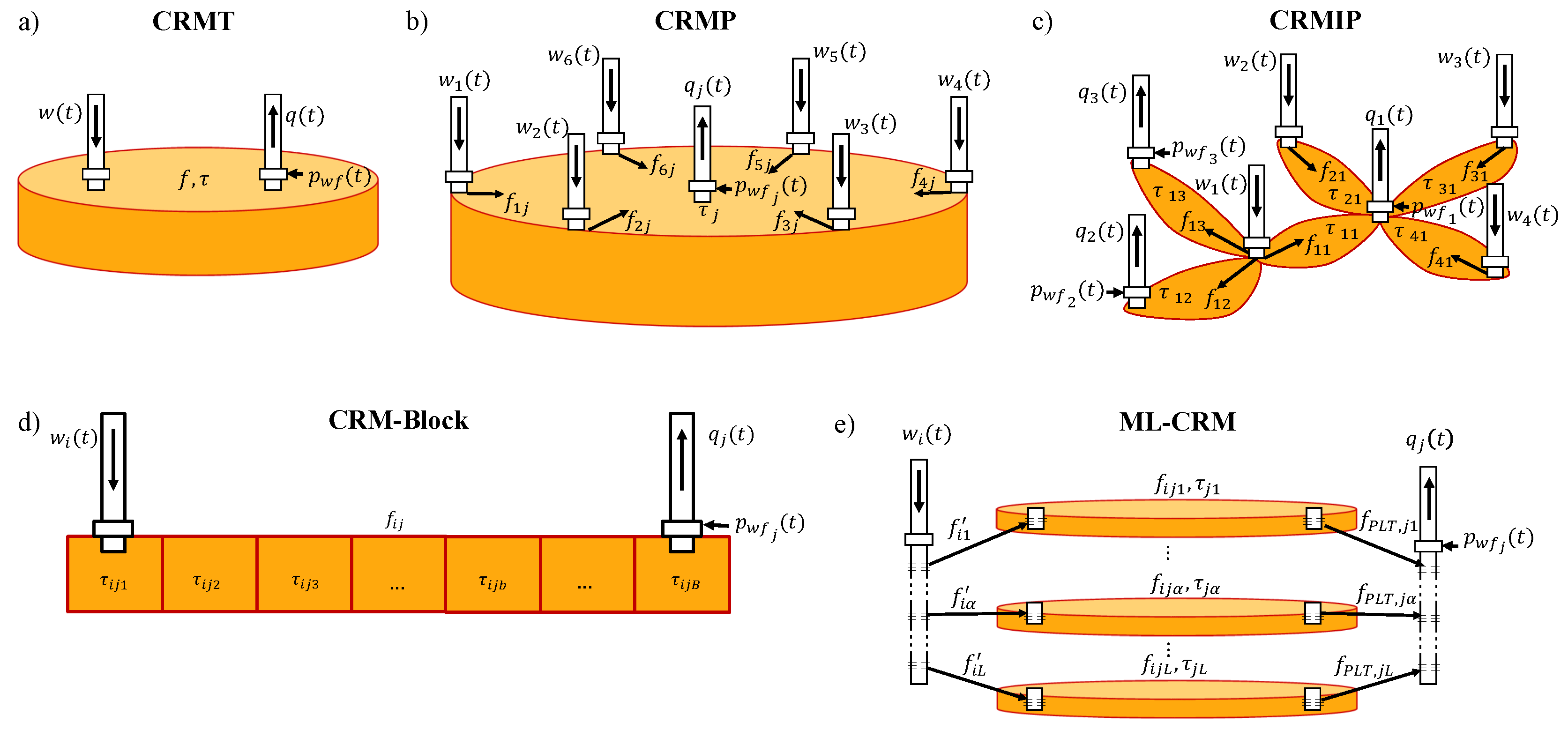
2.1.1. CRMT: Single Tank Representation

The CRMT is defined by the drainage volume of the entire reservoir (Figure 4a) or a specified reservoir region including several injectors and producers. Material balance is computed assuming only a single pseudo-producer and a single pseudo-injector, which sum up all of the respective rates [9]. The parameter f (also known as interwell connectivity, gain, or injection allocation factor) is introduced to Equation (3) to account for the effects of leakage ( f < 1 ), aquifer pressure support ( f > 1 ), or communication between reservoirs [18,19], resulting in the following ordinary differential equation (ODE):
τ d q ( t ) d t + q ( t ) = f w ( t ) τ J d p w f ( t ) d t .
In the case of multiple producers, it may not be trivial to define representative BHP values for the pesudo-producer when BHPs are varying independently. Sayarpour et al. [9] considered the pseudo-producer’s BHP constant, removing the term τ J d p w f ( t ) d t in Equation (6). Alternatively, Kaviani et al. [20] proposed a more robust approach for the case of unknown BHP measurements, the segmented CRM is capable of identifying the times and the magnitude of the effects of producers’ BHP variations on q ( t ) . A third approach is to estimate the pseudo-producer’s BHP as the average of the BHPs converted to the same datum depth [21].
The CRMT concept originated from the analytical model of Fox et al. [18], which was derived to quantify communication between reservoir compartments assuming steady-state single-phase flow. Fox et al.’s [18] methodology was applied to North Sea fields to characterize the flow paths (f), drainage volumes ( V p ), well productivity indices (J), and to determine the use of artificial lift. The CRMT is known as the single tank representation because Equation (6) is analogous to the classical chemical engineering first-order tank model, which is used to predict and control the level of an incompressible fluid within a tank through its inlet and outlet rates [22].
Similar to Equation (5), Sayarpour [12] derived an analytical solution for the ODE of the CRMT (Equation (6)), which is the superposition in time of three factors: primary production, injection, and BHP variation. Likewise, Sayarpour [12] also introduced analytical solutions for CRMP, CRMIP and CRM-block (Figure 4), and these representations are presented in the following sections.
The CRMT allows rapid history matching and prediction at a field scale. Its estimated parameters might provide insight into the effective injection in the reservoir regions, as well as they might be a low cost and useful initial guess for other more robust representations. However, representations that allow computation of individual well flow rates, as opposed to a single pseudo-well, are required for the purposes of understanding flow patterns and optimizing reservoir hydrocarbon recovery, as discussed in the following sections.

2.1.2. CRMP: Producer Based Representation

The reservoir control volumes in the producer based representation (CRMP) are defined as the drainage volume of each producer including all of the injectors that influence their production rates, as shown in Figure 4b. Unless some spatial window is defined [23], all injectors can potentially influence a producer. The CRMP was originally introduced by Liang et al. [8] (see also Liang [24]).
The CRMP assigns one time constant ( τ j ) for the drainage volume of each producer and one connectivity ( f i j ) for each injector (i) – producer (j) pair; therefore, the continuity equation for producer j becomes:
τ j d q j d t + q j ( t ) = i = 1 N i n j f i j w i ( t ) τ j J j d p w f , j d t .
In Equation (7), the main difference from Equation (3) is the first term on the right side, which is the total injected rate from the N i n j injectors that affect producer j. Since only one time constant is assigned for each producer, the CRMP assumes that the production rate will respond with the same time constant to changes in w i ( t ) for all of the N i n j injectors, but with different gains ( f i j ). For this reason, the CRMP is not recommended for very heterogeneous reservoirs, working better when near-homogeneity is present close to the producers and all injectors are at similar distances from the producer, such as for a patterned waterflood.

2.1.3. CRMIP: Injector-Producer Pair Based Representation

The injector–producer pair based representation (CRMIP) assigns one time constant ( τ i j ) and one connectivity ( f i j ) for each injector(i)-producer(j) pair, as shown in Figure 4c, mitigating the problem mentioned above but increasing the number of parameters. This model was first proposed by Yousef et al. [7], and the continuity equation for each control volume is similar to Equation (3):
τ i j d q i j d t + q i j ( t ) = f i j w i ( t ) τ i j J i j d p w f , j d t ,
where q i j is the production rate in producer j from the injector(i)–producer(j) pair control volume, as well as J i j is the productivity index associated with such a control volume. Then, superposition in space is applied to obtain the total production rate of each producer, i.e., the contributions from all of the injectors are summed up:
q j ( t ) = i = 1 N i n j q i j ( t ) .
There are some significant differences between the analytical solutions of Sayarpour et al. [9] and the one originally presented by Yousef et al. [7]. The use of Sayarpour et al.’s [9] solution is recommended in cases where it is not desired to restrict the primary depletion and BHP term to an exponential decline, but to a sum of exponential terms at the expense of estimating more productivity indices.

2.1.4. CRM-Block: Blocks in Series Representation

The first-order tank formulation assumes immediate response to variations in the injection rates. In order to overcome this limitation, Sayarpour [12] (Section 3.5) extended the CRMT and CRMIP to consider the time delay in the producers response. Hence, the injector–producer control volume was divided in several blocks, as a tanks in series model (Figure 4d). This representation was called CRM-block and is recommended for cases with high dissipation, such as low permeability, high frequency injection signal, and/or distant injector–producer pairs.
Sayarpour [12] (Section 3.5) derived the following analytical solution for the CRMT-block for the case of a single step change in the injection rate and constant producer’s BHP:
q ( t ) = q B ( t 0 ) e ( t t 0 ) τ B + b = 1 B 1 q b ( t 0 ) e ( t t 0 ) τ b a = 1 B b ( 1 e ( t t 0 ) τ a ) + w ( t ) b = 1 B ( 1 e ( t t 0 ) τ b ) ,
where B is the total number of blocks between the pseudo-injector and pseudo-producer. This solution was extended to the CRMIP-block representation including the interwell connectivities in the injection term, accounting for the number of blocks between each injector–producer pair ( B i j ), and summing the production rates of the control volumes associated to a producer:
q j ( t ) = i = 1 N i n j q i j ( t ) = i = 1 N i n j q i j B i j ( t 0 ) e ( t t 0 ) τ i j B i j + i = 1 N i n j b = 1 B i j 1 q i j b ( t 0 ) e ( t t 0 ) τ i j b a = 1 B i j b ( 1 e ( t t 0 ) τ i j a ) + + i = 1 N i n j f i j w i ( t ) b = 1 B i j ( 1 e ( t t 0 ) τ i j b ) .
Holanda [25] (Section 3.2.4) derived the transfer function for the CRMIP-block representation accounting for variable producers’ BHP. This approach enables the application of these models in cases of multiple variations in the injection rates and producers’ BHP without requiring long analytical derivations from higher-order linear ODE’s. An alternative approach is to introduce a time lag in a first-order transfer function (single-tank) instead of using higher-order transfer functions (tanks in series) [26].
Although the CRM-block representation is important from a conceptual point of view, showing that it is always possible to increase model complexity, this model has only been applied in a few studies [27,28]. This indicates that, in general, it is not an attractive solution in the pursuit of a simplified reservoir model. One practical issue is the significant increase in the number of parameters. To mitigate this problem, Sayarpour [12] suggests to consider an equal time constant ( τ b ) for all blocks and adjust the number of blocks (B) in the history matching. However, this approach generates another issue because many history matching problems have to be solved to select the most appropriate model. Additionally, pressures and rates of the blocks cannot be attributed to particular reservoir regions, as these control volumes are not spatially defined. In other words, the CRM-block concept is set mainly to mimic the lag in the production response.

2.1.5. Multilayer CRM: Blocks in Parallel Representation

It is common to have impermeable layers interbedded in the reservoir rock, hence modeling the fluid flow to the wells in a compartmentalized manner is more realistic than assuming a single layer, as in the previous representations. Furthermore, production logging tools (PLT) enable detection of the fraction of the total flow coming from each compartment for each producer, i.e., for the α -th layer, q j α = f P L T , j α q j . On the other hand, the injection rate distribution profile for such compartments usually are not inferred, which is a critical control for hydrocarbon recovery optimization. Based on these facts, Mamghaderi et al. [29] proposed a multilayer CRM (or ML-CRM, Figure 4e), which couples PLT data with the CRMP to infer the injected fluid allocation to each layer. In this case, it is necessary to define two levels of allocation factors: (1) f i α represents the fraction of injected fluid from injector i allocated to layer α ; (2) f i j α represents the fraction of f i α w i allocated to producer j.
In contrast to Mamghaderi et al. [29], Moreno [30] generated an ML-CRMP representation assuming that the injection profile ( f i α ’s) is known and the production in each layer is unknown. This is plausible in the case of smart injection wells, but no smart production or PLT data ( f P L T , j α ’s) are available. Moreno [30] presented two formulations for the ML-CRMP: (1) assigning different τ j α ’s for the layers, i.e., each producer has one time constant per layer; (2) assigning a single time constant ( τ j ) for each producer, resulting in a significant reduction in the number of parameters. Although it is reasonable to expect different time constants for the layers due to their distinct properties, Moreno’s [30] case study suggested that, in mature fields, both approaches provide similar accuracy because the reservoir fluids are nearly incompressible. Additionally, the production response is more sensitive to variations in f i j α ’s than in τ j α ’s [31,32,33]. Therefore, in many cases, the second approach may be a valid strategy to reduce the number of parameters for the history matching.
As presented in the model of Mamghaderi and Pourafshary [34], the complexity of the ML-CRM increases significantly when reservoir layers are not separated by completely sealing rocks, but in hydraulic communication, resulting in cross-flow between the control volumes. Zhang et al. [35] complemented the previous models by considering also the case of known injection and production per layer and varying producers’ BHP.
The ML-CRMs previously mentioned extended the CRMP material balance (Equation (7)) to each layer ( α ), such that these models can be summarized as follows:
τ j α d q p , j α d t + q p , j α ( t ) = i = 1 N i n j f i α f i j α w i ( t ) τ j α J j α d p w f , j d t ,
where q p , j α is the total production rate contributed from layer α disregarding the crossflow ( Q c , j α , contribution from other layers), and is related to the observed total production rate in layer α ( f P L T , j α q j ( t ) ) by:
q p , j α ( t ) = f P L T , j α q j ( t ) Q c , j α ( t ) .
The following constraints are necessary for mass conservation:
α = 1 L f i α = 1 ,
α = 1 L f P L T , j α = 1 ,
α = 1 L Q c , j α ( t ) = 0 .
Equation (16) was introduced by Zhang et al. [35] to take into account that the crossflow fluid leaving a layer ( Q c , j α ( t ) < 0 ) must be entering another ( Q c , j α ( t ) > 0 ).
Although Mamghaderi and Pourafshary [34] and Zhang et al. [35] presented formulations that contemplate the cases of crossflow between layers, one must be careful while increasing model complexity. As the number of parameters increase, there will be more combinations that satisfactorily fit the history matched data, and the risk of many of these models providing a poor forecast also increases. Furthermore, the progression of crossflow terms in time may not be properly captured by this approach.
In addition to the previously mentioned references, recent developments and applications of ML-CRMs can be found in [36,37,38,39].

2.2. CRM Parameters Physical Meaning

2.2.1. Connectivities

The interwell connectivity, f i j , also known as gain or allocation factor, is defined by the volume fraction of injected fluid from injector i that can be attributed to the production at well j. Therefore, at stabilized flow conditions, an increase in the injection rate by Δ w i corresponds to an increase in the total production rate by Δ q j = f i j Δ w i in reservoir volumes (Figure 5a). This information is essential for improved management in secondary and tertiary recovery processes, providing an understanding of the reservoir behavior and response to control variables.
Albertoni and Lake [40] inferred interwell connectivities in the cases of balanced and unbalanced waterflooding by correlating injection and production rate fluctuations via a multivariate linear regression (MLR) model. They used diffusivity filters to account for the time lag in the production response. The MLR model was a precursor for the CRM presented by Yousef et al. [7]. Analogously to the Albertoni and Lake [40] model, Dinh and Tiab [41] used only BHP fluctuation data to estimate interwell connectivities via an MLR, without requiring diffusivity filters.
Gentil [42] interpreted the regression coefficients (interwell connectivities) of the MLR model for patterned waterfloods as the ratio of the average transmissibility ( T i j ) between injector (i) and producer (j) to the sum of the transmissibilities between injector (i) and all producers:
f i j = T i j j = 1 N p r o d T i j .
Even though such physical meaning has been extended to the gains ( f i j ) in the CRM literature, one must be aware that it is applicable to patterned mature waterfloods when the injection rates and producer’s BHP are approximately constant and there are no significant changes in the flow pattern, which is a very restrictive condition. In addition, the injector–producer transmissibilities ( T i j ’s) have not been quantified, and Equation (17) has been used more to guide a qualitative interpretation. Since the interwell connectivity is defined as a fraction of the flow rates, a more consistent theoretical equation is proposed here:
f i j = T i j Δ p i j j = 1 N p r o d T i j Δ p i j .
The following material balance constraint is a consequence of the physical meaning of the interwell connectivities:
j = 1 N p r o d f i j 1 ,
where the summation above is less than unity if fluid is being lost to a thief zone, and equal to unity otherwise. Injected fluid might also be lost due to water flowing to the region below the water-oil contact (WOC), to an aquifer, to underpressured reservoir layers, or even to other communicating reservoirs, resulting in inefficient injection.
Regarding the dynamic behavior of f i j ’s, they tend to be approximately constant after water breakthrough, unless there are major perturbations to the streamlines, such as shut-in wells and large variations in injection rates and producer BHPs. This point is exemplified by Jafroodi and Zhang [31] for a regular waterflooding and Soroush et al. [43] for a heavy oil waterflooding cases. Such observation can also be extended to the τ i j ’s and J i j ’s. Therefore, after water breakthrough, the parameters in the CRM governing ODEs (Equations (6)–(8) and (12)) are frequently considered constant, resulting in a linear ODE.
One of the assumptions in the CRMs previously presented is that there is a constant average-reservoir fluid density that represents the system. This is valid in a mature waterflooding because water is slightly compressible and there are slight changes in the saturation. However, before water breakthrough, this assumption is less likely to be valid due to the sharp change in saturation in the water front and significantly higher compressibility of the oil phase. Izgec and Kabir [44] extended the CRMs’ applicability to prebreakthrough conditions by incorporating a pressure-dependent fluid density function to Equation (1), obtaining:
c t V p d p ¯ d t = ρ w , i n ρ ¯ w w ( t ) ρ o , o u t ρ ¯ o q o ( t ) ,
where ρ ¯ w and ρ ¯ o are the average densities of water and oil in the control volumes, respectively, ρ w , i n is the input water density, ρ o , o u t is the output oil density and q o ( t ) is the oil production rate (res bbl/day). Since water is slightly compressible, it is plausible to assume ρ w , i n ρ ¯ w = 1 .
Izgec and Kabir’s [44] approach enables one to gain connectivity information during the early stage of a flooding process. In this sense, CRM serves as a diagnostic tool that allows remedial actions regarding injected fluids’ allocation, avoiding early breakthrough and reducing volumes lost to thief zones, as well as providing a clue for future well placements.

Aquifer–Producer Connectivity

If there is an aquifer providing extra pressure support to the reservoir, the best approach is to couple CRM with an aquifer model in order to account for the controllable (injection rates) and uncontrollable (aquifer) influxes separately. Izgec and Kabir [45] applied the Carter–Tracy aquifer model to estimate the instantaneous water influx and added it to the allocated injection in the CRMP equation ( i = 1 N i n j f i j w i ( t ) + w a j in Equation (7). Their approach accounts for nonuniform support to the producers by attaching a different aquifer model to each producer, resulting in a large increase in the number of parameters (three per aquifer). The strategy adopted to reduce the number of parameters is to define certain regions with common porosity, permeability and thickness, while the drainage radii are computed individually for each producer. Izgec [46] proposed a simplified CRM-aquifer approach assuming a single aquifer connected to a tank. First, the CRMT is coupled with the Carter–Tracy aquifer model to estimate the field instantaneous water influx. Second, the CRMIP is coupled with the single aquifer model and aquifer–producer connectivities ( f a j ) are established to account for the additional influx ( f a j w a j ). The cases of early injection pose an additional difficulty to characterize the aquifer, since the scenarios of high volumes lost to thief zones with large aquifer or low volumes lost to thief zones with small aquifer might both honor the material balance. Izgec [46] suggests generating equiprobable realizations to mitigate this problem.

Comparisons of CRM Interwell Connectivities with Streamline Allocation Factors

Izgec and Kabir [44] and Nguyen [47] provide an interpretation of the interwell connectivity using streamlines. According to their results, f i j ’s are a proxy for streamline allocation factors, which are defined as the fraction of injected fluid conducted by the streamtubes starting at injector i and ending on producer j. Therefore, any change in the streamlines (e.g., caused by fluctuating rates and BHPs or well shut-in) results in varying allocation factors. As depicted by Izgec and Kabir [44], the constant values obtained from the CRM history matching correspond to average values within the time span analyzed.
Although frequently CRM-derived interwell connectivities resemble streamlines allocation factors, these values might be noticeably different for some injector–producer pairs. Therefore, it is important to emphasize that the CRM-derived interwell connectivities are mainly related to the pressure support while streamlines allocation factors are related to the fraction of injected fluid flowing towards a producer. As recently exemplified and discussed by Mirzayev et al. [48] for waterflooding in tight reservoirs and by Holanda et al. [33] for conventional reservoirs, these differences can be further explored when studying the distribution of flow paths and barriers in the reservoir.

Connectivity Interpretation within a Flood Management Perspective

The field studies developed by Parekh and Kabir [49] are useful to illustrate the concepts of interwell and inter-reservoir connectivities and their application to reservoir management. The CRM derived f i j ’s corroborated tracer testing results. The understanding gained from reservoir connectivity can often be tied to the geological characteristics which control hydrocarbon recovery. For example, high permeability pathways, such as fractures, can cause a rapid water breakthrough in a producer (high f i j ) or water leaking to a thief zone (low f i j ), and both cases are associated with poor sweep-efficiency, requiring redesign of the flooding process (e.g., choose a more efficient EOR fluid). Parekh and Kabir [49] also suggest a methodology to analyze thief zones applying a water-oil ratio (WOR) plot, a modified-Hall plot, 4D seismic, rate transient analysis and the CRM.
Thiele and Batycky [50] defined injection efficiency as the volume ratio of incremental oil obtained by fluid injected. Their empirical management approach consists of assigning gradually increasing flow rates to more efficient injectors and reducing it to the less efficient ones based on an established equation. This is applied sequentially, updating injection efficiencies and allocation factors every time step via streamlines simulation. Instead of using numerical optimization, their method exemplifies how streamline allocation factors and water-cut information can improve waterflooding management solely by simple reservoir engineering judgments. As it will be discussed in Section 2.4, f i j ’s can be updated sequentially via ensemble Kalman filters; this allows the use of Thiele and Batycky’s [50] method with the CRM.

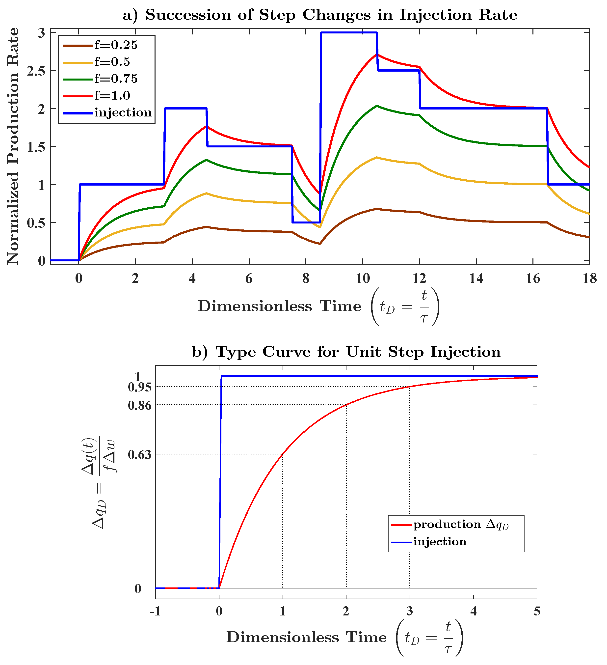
2.2.2. Time Constants

The CRM time constant, previously defined in Equation (4), accounts for dissipation of the input signals in the porous media; these input signals are injection rates and producer BHPs which are varying in time. As previously mentioned, τ is also related to the production decline during primary recovery. In fact, τ ’s are intrinsically associated with pressure diffusion, while time of flight in streamlines simulation is associated with the evolving saturation of the phases. If a step increase is applied to injection rates in the CRMT, CRMP, CRMIP or ML-CRM (first order systems), one time constant ( t = τ ) is the time to achieve 63.2% of the final production rate; 95.0% is achieved at t = 3 τ (Figure 5b).
A straightforward analysis of Equation (4) shows that a large pore volume ( V p ), a very compressible system ( c t ) and/or a low productivity index ( J ) results in a large τ , and therefore large dissipation of the input signals and slow decline of the primary production term. In contrast, a fast transmission of the input signals and fast decline of the primary production term results from small τ , which is obtained in the cases of small pore volume ( V p ), low total compressibility ( c t ) and/or high productivity index ( J ).
For an overview on the physical meaning of productivity indices and models, the reader is referred to [51].

2.3. CRM for Primary Production

As presented in the works of Nguyen et al. [10] and Izgec and Kabir [11], the continuity equation (Equation (3)) is simplified in the case of primary production by assigning w ( t ) = 0 . The formulations presented in these works permit quantification of the drainage pore volumes ( V p j , if c t is known) and productivity indices ( J j ) of each producer, as well as average compartment pressure ( p ¯ ( t ) , from Equation (2)) only from the primary production decline and BHP fluctuations. These simple methods are an alternative to the traditional build-up test with the advantage that no shut-in time is required, therefore production is not delayed, and can be easily applied to multiwell systems without requiring prior knowledge of the reservoir properties (such as porosity, permeability and thickness). Izgec and Kabir [11] extended the application of this method to gas wells by using pseudopressure functions.
Nguyen et al. [10] applied the CRM integrated form (ICRM, to be discussed in Section 2.4) in a sequential manner (piecewise time windows) to identify the increasing drainage volume during transient flow until the onset of pseudosteady-state (PSS), when V p j tends to be constant, as well as a reduction in V p j due to infill drilling. Varying BHPs of neighboring wells and workovers also change the no flow boundaries and consequently V p j ’s. Izgec and Kabir [11] used longer time windows, suggesting to use only PSS data, and validated the drainage volume results with the ones obtained via streamlines simulation. In addition, Izgec and Kabir [11] qualitatively inferred interwell connectivity and reservoir compartmentalization by analyzing V p j ’s before and after drilling new wells.
The evolving behavior of V p j ’s and pressure depletion during primary production are valuable information for reservoir management that can be obtained via these methods. However, neither study provided a robust model capable of predicting the time-varying behavior of V p j , which could lead to a more effective BHP control, for example; this should be the subject of future research.

2.4. CRM History Matching

CRMs are generated through history matching, where the model parameters are adjusted so that the total flow rates predicted by CRM “fit” the observed production history. This is essentially an optimization problem where many types of objective function can be chosen to penalize the mismatches; the following least squares function is a common choice:
min z = min ( q pred q obs ) T C e 1 ( q pred q obs ) ,
where q pred and q obs N t N p r o d × 1 and are the vectors of predicted and observed, respectively, total fluid rates for all of the wells and at every time step; C e N t N p r o d × N t N p r o d and is the covariance matrix of the measurement and modeling errors; N t is the number of time steps. q pred is computed from the solution of the CRM representation (e.g., Equation (5)).
In fact, many studies do not explicitly consider the matrix C e in the objective function, e.g., [7,12,30,52]. The following publications offer alternative formulations:
  • Holanda et al. [33] considered C e as a diagonal matrix considering each diagonal element proportional to q obs 2. This is equivalent to assume that the errors are independent and proportional to q obs , as a simplifying assumption. In this case, the objective function becomes the relative squared error instead of the absolute squared error. Additionally, a minimum value is set to the q obs 2 diagonal elements of C e to avoid overfitting lower rates because when q obs approaches zero, a high relative error may correspond to an acceptable absolute error. Their results indicated that this approach improved the quality of the history matching.
  • Holanda et al. [53] applied weights to the diagonal elements of the previous formulation [33]. These weights were defined by heuristic rules aiming to select the most representative data to forecast production with a decline model. Such heuristic rules can be adjusted to improve the probabilistic calibration in large datasets.
For a theoretical discussion on modeling and measurement errors and algorithms for nonlinear inverse problems, the reader is referred to Chapter 8 of Oliver et al. [54].
While history matching data, it is necessary to restrict the solution space to physically plausible values of the parameters. Therefore, Equation (21) is subject to several constraints:
min χ z ( χ ) such that a · χ b , a eq · χ = b eq , l b χ u b ,
where χ is the vector of parameters (e.g., f, τ and J); z ( χ ) is the objective function (scalar, Equation (21)); a and a eq are matrices, b and b eq are vectors for the inequality and equality linear constraints, respectively; and l b and u b are lower and upper bounds of the parameters, respectively. Holanda [25] and Holanda et al. [52] present the structure of these matrices for the CRMT, CRMP and CRMIP representations. Equation (19) is an inequality constraint that is valid for all representations, Equation (9) is an equality constraint for the CRMIP and Equations (14)–(16) are equality constraints for the ML-CRM.
There are several optimization algorithms capable of solving the problem stated by Equations (21) and (22). It is beyond the scope of this paper to discuss the mathematical formulation as well as the advantages and disadvantages of each. Instead, the reader is referred to a comprehensive literature review on reservoir history matching by Oliver and Chen [55]. For reference, Table 1 briefly highlights some aspects of several algorithms and their application to CRM history matching.
Probabilistic history matching allows obtaining multiple CRM realizations to analyze the uncertainty in the parameter estimates and production forecast. For this purpose, Kaviani et al. [32] used the bootstrap, which is a sampling with replacement method. Sayarpour et al. [59] history matched multiple realizations of CRM with a Buckley–Leverett-based fractional flow model (Section 3) starting from different initial guesses. Their main objective was to assess the uncertainty in reservoir parameters such as porosity, irreducible-water and residual-oil saturations. Holanda et al. [53] used a Bayesian framework with the Markov chain Monte Carlo algorithm for production data analysis in unconventional reservoirs.

2.4.1. Dimensionality Reduction

Table 2 shows the number of parameters to be estimated for each CRM representation. As the number of parameters increase, issues with the non-uniqueness of the history matching solution become more concerning, so it is important to gather more data (e.g., tracer and interference tests, PLT and smart completions data for the multilayer reservoirs) and/or measure at a higher frequency to reduce ambiguities. It is also highly recommended to consider dimensionality reduction techniques, which can reduce the impact of spurious correlations within the production data in the model fitting. The following are examples of such techniques:
  • Define a spatial window of active injector–producer pairs based on the interwell distance and reservoir heterogeneity, f i j = 0 for wells outside the spatial window [23];
  • Define a maximum number of nearest injectors that could affect a producer well [57];
  • Assign the same τ j to all layers in the ML-CRM [30];
  • Instead of applying the CRM-block representation, i.e., blocks in series, use a first-order tank with a time delay [26];
  • Assign a single productivity index per producer in the CRMIP representation [60].

2.4.2. Alternative CRM Formulations

Besides defining which optimization algorithm and dimensionality reduction technique are suitable for application, it is also important to be aware of alternative CRM formulations that may facilitate the history matching under specific circumstances.

Matching Cumulative Production: The Integrated Capacitance Resistance Model (ICRM)

The integrated capacitance resistance model (ICRM) is based on the same control volume as the CRMP; however, the ODE is integrated providing a linear model for cumulative production [10,61,62]:
N p , j k = ( q j 0 q j k ) τ j + i = 1 N i n j f i j W i k + J j τ j ( p w f , j 0 p w f , j k ) ,
where N p , j k is the cumulative total liquid production of producer j at end of the k-th time step ( t k ), and W i k is the cumulative volume of water injected in injector i at t k . In this case, the history matching is performed for the cumulative total liquid production. The advantage of curve fitting a linear model is that there is a unique solution which is obtained in a finite number of iterations, so it is computationally very fast, and it is easier to determine confidence intervals for the parameters. On the other hand, the cumulative production is smoother than rates and always increases with time, so mismatches in the last data points of the production history may be penalized more than the early ones and overfitting may be an issue. To mitigate these problems, Holanda et al. [33] proposed a normalization of the ICRM history matching objective functions based on the propagation of error of individual rates in the cumulative production; the results presented for two reservoirs showed better agreement with the connectivity estimates from CRMP and CRMIP.
Laochamroonvorapongse et al. [13] suggest that, even if the nonlinear models are applied, an improvement in the quality of the history matching solution is obtained by first matching CRM production rates, then using the solution as an initial guess for the matching of CRM cumulative production. Another approach to determining initial guesses is to use the gains calculated from the case of a homogeneous reservoir, as described by Kaviani and Jensen [63].

Unmeasured BHP Variations: The Segmented CRM

Situations where producers’ BHP data are not available or not measured with the appropriate frequency are common. In these cases, the assumption of constant BHP may not be plausible, so it is important to account for BHP variations while history matching models even if they are unmeasured. The segmented CRM [20,64] is a model proposed for the detection and quantification of the effects of such unmeasured BHP variations:
q j ( t n ) = q j ( t 0 ) e t n t 0 τ p j + i = 1 N i n j k = 1 n f i j e t n t k τ i j ( 1 e Δ t k τ i j ) w i ( t k ) + q B H P j ( T s ) ,
where q B H P j ( T s ) is a constant added to the analytical solution that accounts for the unknown BHP variations in the segmented time T s and is a parameter included in the history matching. Kaviani et al. [20] proposed an algorithm for the identification of the segmentation times, i.e., when the producer BHP changes significantly.

Changes in Well Status: The Compensated CRM

A common assumption of most CRM representations is a constant number of active producers; however, well status changes may occur frequently in the field (flowing, shut-in, and conversions from producer to injector). Therefore, specific strategies must be pursued for history matching in these cases to avoid redefining a time window and reestimating all of the parameters every time there is a change in well status. Significant changes in flow patterns and allocation of injected fluids are expected as wells are shut or opened. The compensated CRM [20,64] uses the superposition principle to treat shut-in producers as a combination of two wells: the actual producer with open status and a virtual injector that re-injects all of the produced fluid at the same location. Considering constant producers’ BHP, the analytical solution for the compensated CRM is:
q j v ( t n ) = q j ( t 0 ) e t n t 0 τ p j + i = 1 N i n j k = 1 n f i j v e t n t k τ i j v ( 1 e Δ t k τ i j v ) w i ( t k ) ,
where the subscript v indicates that the v-th producer is shut-in. In this case, the interwell connectivities are redefined as:
f i j v = f i j + λ v j f i v ,
where λ v j is the interwell connectivity between the virtual injector equivalent to the v-th producer. In other words, the λ v j also measures the producer–producer connectivity observed by the change at well j when well v is shut-in. Thus, λ v j ’s and τ i j v ’s are additional parameters estimated during the history matching. As mentioned by the authors, this model is also useful when producers are converted to injectors.

2.5. CRM Sensitivity to Data Quality and Uncertainty Analysis

As studied by Tafti et al. [65], the identification of the CRM parameters and their underlying uncertainty are intrinsically related to:
  • the amplitude and frequency of uncorrelated variations in the input signals (injection rates and producers’ BHP) because the most relevant dynamic aspects of the system must be observed in the output signals (production rates);
  • the amount of data available for history matching, i.e., sampling frequency (e.g., whether production data are reported daily or monthly) and length of the history matching window;
  • the properties of the reservoir system, such as permeability distribution, fluid saturation and total compressibility.
Originally, the CRM was developed as a dynamic reservoir model with interwell connectivities estimated from variations in the production and injection data that commonly occur in field operations. Thus, ideally, it would not be necessary to change injection rates or producers’ BHP merely for the identification of the CRM parameters. However, if in any circumstances it is desired to improve the information content of the input/output signals, the studies of Tafti et al. [65] and Moreno and Lake [66] provide guidelines based on systems identification theory. The approach developed by Tafti et al. [65] relies on previous information of the systems dynamics, which might be acquired through well test, for example, to define criteria for sampling time, frequency and amplitude of variations and experimental length. On the other hand, Moreno and Lake [66] do not assume a previous knowledge of the reservoir dynamics, and frames the injection scheduling as an optimization problem with an objective function that minimizes the uncertainty in the parameter estimates and the number of changes in injection rates. Their results suggest that bang-bang inputs [67] are optimal in the case of injection rates constrained solely by a maximum and minimum value. If there is a constraint for total water injected in the reservoir or field (linear constraint), it is suggested that piecewise constant signals are optimal.
Kaviani et al. [32] thoroughly analyzed the impact of reservoir and fluid properties and data quality on the accuracy of f i j ’s and τ ’s estimates. The main parameters were: diffusivity constant (i.e., lumped k, ϕ , μ and c t ), number of producers per area ( N p r o d A ), amount of data available and measurement noise. To provide general guidelines regarding the CRMs applicability and expected accuracy of the parameters estimates, the CM (or CRM) number, C, was a new metric introduced, which in field units (see nomenclature section) is:
C = 0.006328 k Δ t N p r o d A ϕ μ c t .
Their analyses of 11 reservoirs indicate that the CRM parameters are accurate and repeatable when CM numbers are in the range 0.3 C 10 . The parameter L was introduced to provide guidelines regarding data sufficiency for the history matching; L is the ratio of total sampled data points ( N t N p r o d ) to the number of parameters ( N p a r , as described in Table 2 if dimensionality reduction is not applied):
L = N t N p r o d N p a r .
According to their results, a minimum value of L = 4 is recommended for consistent estimation of the parameters. Increasing the number of sampled data points improves consistency of the history match even if significant levels of measurement noise occur.
Moreno and Lake [68] derived an analytical equation to quantify the uncertainty in connectivity estimates for the unconstrained history matching problem, and such equation accounts for the information content of the injection signal and levels of measurement noise in the liquid production rates. The estimated uncertainty of the unconstrained problem serves as an upper bound for the constrained history matching. A limitation of their approach is that τ ’s must be known a priori, so it is necessary to perform at least one history match before applying the analytical solution for the upper bound of the f i j uncertainty. The advantage is that it is significantly less computationally demanding than performing uncertainty analysis by sampling (e.g., Markov chain Monte Carlo, bootstrap).
As previously discussed, the reliability of CRM history matched models is highly dependent on the quality and amount of data available. There are several factors that might contribute to problematic data, e.g., measurement noise, sudden variations in operational conditions, partially unrecorded production data, completely missing BHP data, and commingled production. Cao [69] implemented an iterative process for production data quality control based on successive CRM fits to the observed production. The periods of erroneous or missing data are selected. Then, it is replaced by the CRM prediction. This process is repeated until the difference of successive estimated parameters are below a tolerance. One relevant application of this workflow is as a preprocessing step in the history matching of grid-based reservoir models. However, before applying this procedure, one should be cautious and ensure that the CRM is a reliable representation of the reservoir dynamics, i.e., the deviations in the production data are mainly due to problems in the data rather than caused by a physical phenomena that goes beyond CRMs modeling capabilities.

3. Fractional Flow Models

The CRM representations previously presented calculate the liquid production rate of each producer ( q j ). However, it is necessary to separate oil and water production rates ( q o j and q w j ) in order to improve reservoir management and make financial forecasts. A fractional flow model is used for this purpose.

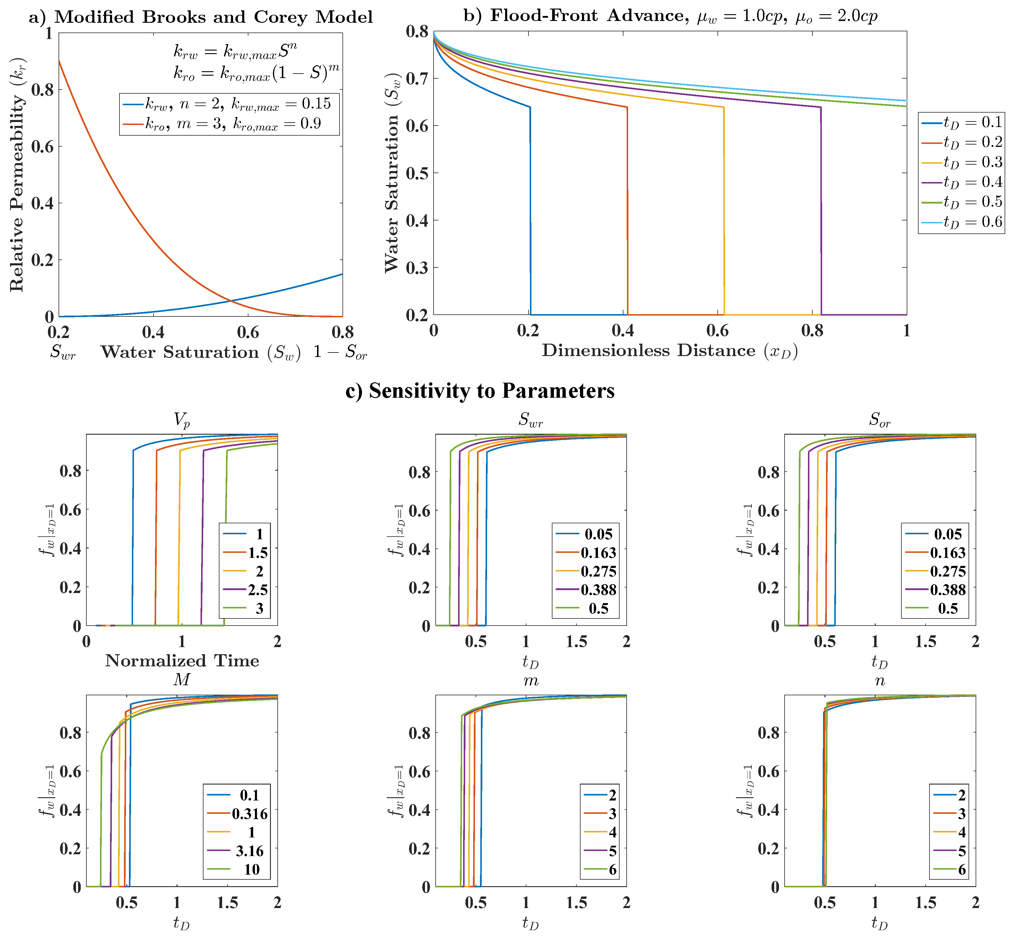
3.1. Buckley–Leverett Adapted to CRM

The Buckley and Leverett [70] physics-based model is probably the most popular fractional flow model amongst reservoir engineers. It assumes linear horizontal flow of immiscible and incompressible phases in a 1D homogeneous reservoir, and neglects capillary pressure and gravitational forces. It allows estimation of the location of the flood-front, saturation profile and water-cut at the producer, given the relative permeability curves and fluid viscosities (Figure 6a,b). Sayarpour [12] presented a fractional flow model based on the one from Buckley and Leverett [70] which can be applied with CRM (see also [59]):
f o ( S ) = 1 1 + ( 1 S ) m M S n 1 ,
where f o is the oil cut (i.e., oil fractional flow at the producer), m and n are relative permeability exponents from the modified Brooks and Corey [71] model (Figure 6a), M is the end-point mobility ratio, and S is the normalized average water saturation, defined as:
S ( t ) = S w ( t ) S w r 1 S o r S w r ,
where S w r and S o r are the irreducible water and residual oil saturations, respectively, and S w ( t ) is the saturation at the outlet of the control volume. However, Sayarpour [12] used the average water saturation in the control volume, which can be computed through the following material balance equation:
S w ( t k ) = S w ( t k 1 ) + w j * ( t k ) q w j ( t k 1 ) V p Δ t k ,
where w j * ( t k ) = i = 1 N i n j f i j w i ( t k ) , which is the effective water injected in the control volume. Additional calculations are necessary to compute S w ( t ) at the outlet of the control volume [70,72], the results for a sensitivity analysis in this case are shown in Figure 6c. This model has six unknowns (m, n, M, S w r , S o r and V p ), so there are many degrees of freedom. As a result, the parameters of a single history matched model may not correspond to the actual reservoir properties and provide a poor forecast. For this reason, Sayarpour et al. [59] used this model mainly for the uncertainty quantification of reservoir parameters ( S w r , S o r and ϕ ) before starting to develop a grid-based reservoir model. An alternative approach to be considered in the implementation of this fractional flow model is to define m, n, M, S w r , S o r as global reservoir variables and only a single V p for each control volume or per producer.

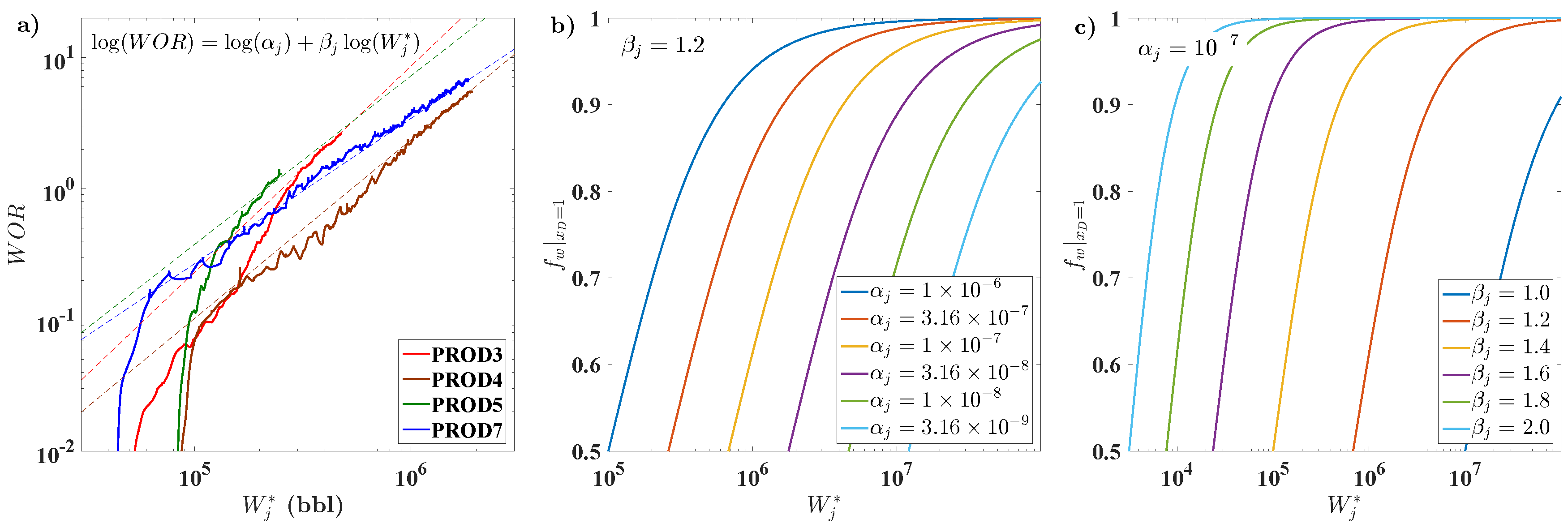
3.2. Semi-Empirical Power-Law Fractional Flow Model

Semi-empirical models are an alternative to reduce the number of parameters while applying a functional form that mimics the observed behavior. For oil cut in an immiscible displacement process, the function must be monotonically decreasing and with values between 0 and 1. The most popular fractional flow model for waterflooding in mature fields is the one based on the power-law relation for water–oil ratio (WOR) derivable from Yortsos et al. [73], rediscovered by Gentil [42], and further developed for CRM by Liang et al. [8]:
f o ( t k ) = q o j ( t k ) q j ( t k ) = 1 1 + α j W j * ( t k ) β j ,
where α j and β j are the fractional flow parameters for producer j, and W j * ( t k ) is the effective cumulative water injected to the control volumes of producer j up to the k-th time step, defined by:
W j * ( t k ) = i = 1 N i n j t 0 t k f i j w i ( ϵ ) d ϵ i = 1 N i n j κ = 1 k f i j w i ( t κ ) .
In order to ensure physically plausible behavior, both parameters are constrained to being positive ( α j , β j > 0 ) so that 0 f o ( t k ) 1 and it decreases with W j * ( t k ) . Besides the fact that it has only two parameters, an advantage of this model is that it can be written as a straight line equation (Figure 7), which facilitates the history matching of oil cut (or oil rates) that can be performed independently for each producer. In addition, the only additional information required after the CRM history matching are the oil rates.

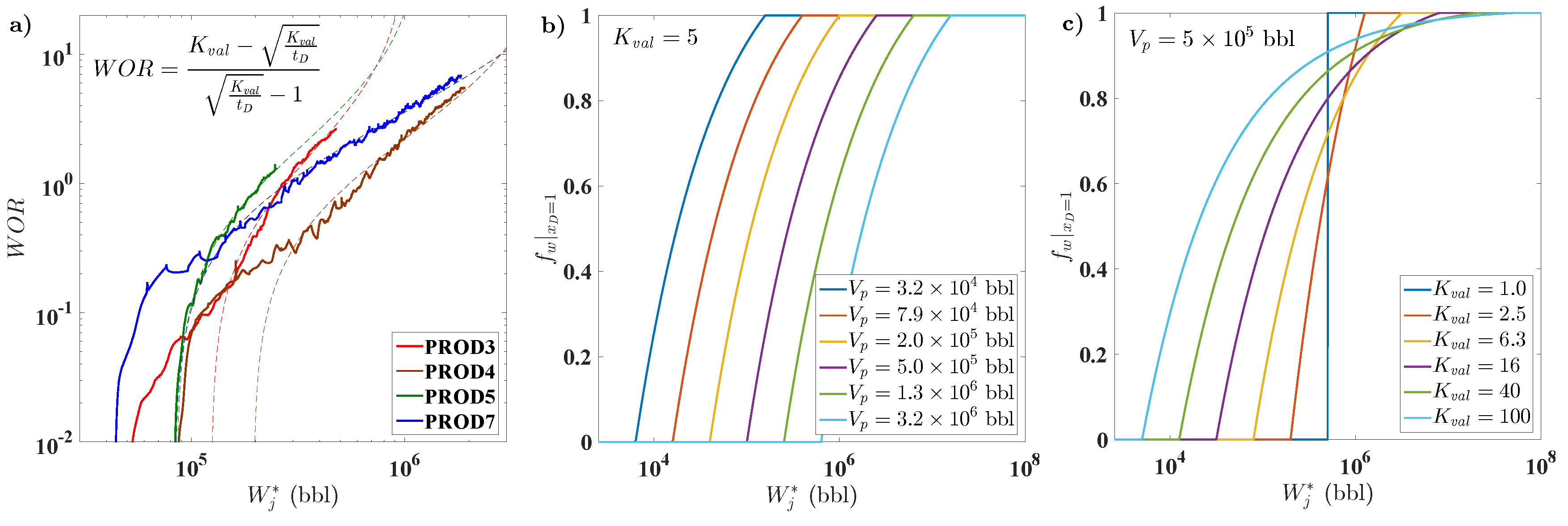
3.3. Koval Fractional Flow Model

In contrast to the semi-empirical power-law model that is applicable for mature fields only (higher values of water cut, e.g., f w 0.5 ), the formulation that couples CRM and the Koval [74] fractional flow model is more suitable to span the whole life of a waterflooding project, i.e., 0 f w 1 [75,76,77]. The Koval model is physics-based and originally was formulated for the miscible displacement of solvent in a heterogeneous media; later, it was proven to be equivalent to the Buckley–Leverett model when the relative permeability curves are straight lines, i.e., m = 1 , n = 1 in Equation (29) [78]. The Koval equation for the fractional flow of water is:
f w = 1 1 + 1 K v a l 1 S S ,
where S is the normalized average water saturation (Equation (30)), and K v a l is the Koval factor:
K v a l = H E ,
where H is a heterogeneity factor ( H = 1 for homogeneous and H > 1 for heterogeneous porous media) and E is the effective oil-solvent viscosity ratio:
E = 0.78 + 0.22 μ o μ s 0.25 4 .
Equations (34)–(36) set the basis of the Koval model. However, they are expressed in terms of saturation which is not directly measured in the field, and μ o , μ s and H may be unavailable. Cao [75] developed the following formulation that is more straightforward for field application when combined with the CRM:
f w | x D = 1 0 , t D < 1 K v a l , K v a l K v a l t D K v a l 1 , 1 K v a l < t D < K v a l , 1 , t D > K v a l ,
where x D is the dimensionless distance (i.e., distance from injector divided by total distance in the control volume), f w | x D = 1 denotes the water fractional flow at the producer, i.e., the water-cut; t D is the dimensionless time, which is the cumulative volume injected to the control volume divided by its total pore volume:
t D = W * ( t ) V p ,
where W * ( t ) is given by Equation (33). For a detailed derivation of Equation (37), the reader is referred to Appendix A of Cao et al. [77].
Therefore, as in the power-law fractional flow model (Equation (32)), there are only two unknowns per producer in history matching of the Koval model ( V p and K v a l ). The advantage is that it can be applied earlier for production optimization in a waterflooding project. Even though the model includes the prebreakthrough scenario ( f w = 0 ), the parameters cannot be identified before the water breakthrough. Figure 8 shows an application of this model and the water-cut sensitivities to V p and K v a l . The pore volume ( V p ) controls the breakthrough time, shifting the water-cut profile in the semilog plot while K v a l defines the shape of the water-cut curve, accounting for heterogeneity and viscosity ratio. K v a l = 1 when μ o μ w = 1 and the reservoir is homogeneous ( H = 1 ); as a result, piston-like displacement is observed.
Cao et al. [76] presented a fully-coupled formulation for the CRM/Koval fractional flow model, which accounts for the effects of the evolution of the water front. As saturation changes, the mobility and total compressibility change accordingly. As a result, the total productivity index and time constants are a function of the average saturation of the control volumes and present a significant time-varying behavior at low water cuts. For a review of other fractional flow models, see Sayarpour [12].

4. CRM Enhanced Oil Recovery

Even though the models presented thus far were mainly developed for waterflooding, the CRM has also been applied to enhanced oil recovery (EOR) processes. In some reports, the models previously presented are used exactly in the same way as in waterflooding, while in others specific developments were carried out to account for the particularities of the EOR process under investigation. This section presents the references and highlights of such developments and applications of the CRM to EOR processes.
In any EOR process, it is critical to understand the displacement efficiency at several scales (e.g., pore, interwell, basin). Yousef et al. [79] proposed a flow capacity plot, which serves as a diagnostic tool for the injection sweep efficiency in the interwell scale. Izgec [46] also presented an application of this concept. In this plot, two measures must be computed from the CRMIP parameters, the cumulative flow capacity ( F m j ) and the cumulative storage capacity ( Φ m j ), which are defined as follows:
F m j = i = 1 m f i j i = 1 N i n j f i j ,
Φ m j = i = 1 m f i j τ i j i = 1 N i n j f i j τ i j .
In these summations, the parameters related to producer j are rearranged in decreasing order of 1 τ i j , thus i = 1 corresponds to the injector–producer pair with smallest τ i j and i = N i n j is the pair with largest τ i j . Figure 9 shows an example of flow capacity plot for four producers in a channelized reservoir. This plot determines how the flow is distributed across the pore volume related to each producer, i.e., the percentage of flow coming from a specified percentage of pore volume. In an ideal displacement, all of the pore volume would be swept evenly. In this case, the curve would fit the unit slope line. Therefore, the deviations of each curve from the 45 line can be related to several types of heterogeneity in the porous media (e.g., fractures, high permeability layers), and serve as a measure of the sweep efficiency of a producer. The closer it is to the 45 line, the more efficient it is. Therefore, the flow capacity plot allows identification of problematic wells that may need an EOR process to effectively mobilize the oil left behind the previous flood front.
Table 3 lists the CRM references by EOR process and provides some highlights on the implementation of each work. Even though the complexity of the physical and chemical interactions between fluids and rock are overlooked by these simple models, generally the published examples present good history matching and prediction when compared to grid-based reservoir simulation and actual field production data. Therefore, the CRM can be a valuable tool in many EOR processes as well, providing insights in the main drives for pressure support, reservoir heterogeneity, and advances of the flood front before more complex and time-consuming simulation models are developed.

5. CRM and Geomechanical Effects

Even though the CRM representations previously shown completely disregard any sort of geomechanical effects, there are occasions when their interference with fluid flow is significant. Subsidence is a well known geomechanical phenomena where the level of a surface decreases, which is mainly due to the displacement of subsurface materials and deformations caused by changes in the effective stress. Subsidence can cause several operational and environmental problems, for example, flooding, damage to surface facilities and well structure, permeability and porosity reduction, and fracture reactivation.
Wang et al. [88] and Wang [89] studied fluid flow and the effects of subsidence in a waterflooding in the Lost Hills diatomite field in California. Diatomites are a fragile formation with high porosity and low permeability. When water is injected at high pressures, the formation is fractured, and high permeability channels are generated. The injected water flows mainly through these channels and a significant amount of oil remains unswept. Additionally, the pressure is lower at these channels, which causes more subsidence. In order to study how fluid flow has been affected by these phenomena, they applied the CRMP in three time windows, which were chosen based on observed large increases or decreases in field injection associated with large changes in subsidence. For a specific region of the field, they observed dramatic changes in the interwell connectivities for each period; with the aid of a polar histogram for f i j ’s, they confirmed that the main directions of flow changed. They also superimposed the connectivities maps with subsidence maps obtained from satellite images, confirming that subsidence was more pronounced in that specific area.
Additionally, Wang et al. [88] and Wang [89] introduced two models to predict average surface subsidence from injection and production data. The linear model accounts for elastic deformation while the nonlinear model accounts for elastic and plastic deformation of the reservoir rock. Unfortunately, the results presented were not satisfactory and have not built the confidence required, which indicates that it is necessary to acquire more information and further develop these ideas. Al-Mudhafer [90] presented a case study using Wang’s linear model for a grid-based reservoir model representing the South Rumaila field in Iraq; however, his results are unclear and seem to lack validation with a more reliable physics-based geomechanical model.
Recently, Almarri et al. [91] presented a study where variations in the interwell connectivities from the CRMIP are used in conjunction with other analytical tools to identify thermally induced fractures, their directions and impact on the flooding front. These fractures are triggered by the lower temperature of the injected water.

6. CRM Field Development Optimization

During field development, there are several variables that can be optimized to meet safety standards, environmental regulations, contractual expectations and/or maximize net present value (NPV). The following are some examples of these variables: botomhole pressures or rates of injectors and producers (well control problem); location and trajectory of new wells to be drilled (well placement problem); EOR fluids to be injected (e.g., type of fluid, concentration, duration and rate of each slug injected); stimulation treatment (e.g., propped volume and number of stages for hydraulic fractures; concentration, injection rates and duration of acidizing treatment). As will be discussed in this section, CRMs are capable of providing solutions for the well control and some insights for the well placement problem.

6.1. Well Control

The control variables in CRM are injection rates and producers’ BHP, all of which are included in the input vector:
u = [ w 1 , , w N i n j , p w f , 1 , , p w f , N p r o d ] T .
The well control problem consists of searching for an optimal control trajectory for all of the wells to achieve a specified objective (e.g., maximum NPV) in a time horizon (e.g., next 10 years). Here, all of the well trajectories are written in a single matrix:
U t = u ( t N t ) , , u ( t k ) , , u ( t N f t ) ,
where t N t is the last time step of the history matching window and t N f t is the last time step of the optimization time horizon.
Once the variables of the problem have been defined, it is necessary to specify the objective function and constraints. As an attempt to maximize profit during oil production, a common objective is to maximize the net present value with CRM and a fractional flow model for prediction:
max U t N P V = max U t k = N t N f t j = 1 N p r o d ω p o q o j ( t k ) ω p w q w j ( t k ) ω i w i = 1 N i n j w i ( t k ) Δ t k ( 1 + r ) k N t ,
where ω p o , ω p w and ω i w are the prices of produced oil, produced water and injected water, respectively; and r is the discount rate per period. Depending on the situation, it might be plausible to include other factors in Equation (43), for example, price of produced gas, drilling and abandonment costs. Several authors have considered the problem of maximizing NPV with CRM [19,31,92,93,94]. Alternative formulations for the objective function include maximizing cumulative field oil production [8,9], and minimizing cumulative field CO 2 production [86].
The following are examples of the constraints that can be considered:
max U t N P V ( U t ) such that p w f , m i n p w f , j p w f , m a x , 0 w i w m a x , 0 N i n j w i w c a p , 0 N p r o d q j q c a p ,
where p w f , m i n and p w f , m a x are the BHP limits to satisfy formation stability and integrity, respectively, w m a x is the maximum injection rate allowed in a single injector, w c a p is the total capacity of the surface facilities to provide the injected fluids to the reservoir, and q c a p is the total capacity of the surface facilities to process the produced fluids.
The dimension of the well control optimization problem defined by Equations (41)–(44) is ( N i n j + N p r o d ) ( N f t N t 1 ) . However, the producers’ BHPs are frequently assumed to be constant and therefore excluded from this problem, which becomes only a matter of reallocation of the injected fluids, reducing its dimensions to N i n j ( N f t N t 1 ) . As suggested by Sorek et al. [95] for well control optimization in grid-based reservoir models, it is possible to drastically reduce the dimension of the problem by parameterizing the control trajectories of each well. In this parameterization, it is important to have an efficient way to span the solution space considering trajectories that are logistically viable. The results obtained by Sorek et al. [96] suggest that the use of Chebyshev orthogonal polynomials as the basis for such parameterization results in faster convergence and higher NPV with smooth trajectories for well control, which is desirable from an operational perspective.
Once the optimization problem has been defined (objective function, constraints and variables), it is necessary to choose a suitable algorithm capable of maximizing (or minimizing) the objective function honoring the constraints, and preferably performing at a reduced computational time. A discussion on the applicability and mathematical formulation of optimization algorithms is beyond the scope of this paper. However, it is worth mentioning some algorithms that have been applied to the CRM well control optimization problem: sequential quadratic programming [8], generalized reduced gradient algorithm [9,92], genetic algorithm [29], and ensemble optimization [31,93,94].
In closed-loop reservoir management, the models are gradually updated as more information is acquired. Then, these updated models are used to predict reservoir dynamics, and optimize well control for the next time steps. Jafroodi and Zhang [31] and Stensgaard [93] presented a framework for closed-loop reservoir management using CRM as the reservoir model. Since CRM predicts production rates by solving a continuity equation for a reduced number of control volumes when compared to grid-based reservoir simulation, it is expected to drastically reduce the computational time in these recursive optimization problems. Hong et al. [94] discussed the use of CRM as a proxy model for waterflooding optimization in the cases where a grid-based reservoir model is available; their results indicate that CRM provides a near-optimal solution when compared to the more descriptive grid-based models.

6.2. Well Placement

As previously discussed in Section 2.4, the CRM and fractional flow parameters are obtained from history matching the production rates. If a well has not been drilled and produced or injected for a significant period yet, data is not available, and the CRM parameters cannot be inferred. For this reason, usually CRM is not used to optimize well placement. Nonetheless, it is worth mentioning the efforts of two works in this subject [19,97].
Weber [19] proposed two methods for the injector well placement problem. The first one creates a simple grid-based reservoir model to generate several simulation results (pseudo-data) with wells at different locations. Then, CRM and fractional flow models are history matched and the parameters affected by the new well are mapped onto a surface, which is approximated by an equation (e.g., a plane). After this parameterization, the well placement problem is solved using a mixed integer nonlinear programming algorithm, where the discrete variables define the well status at all available locations. Ideally, a reduced number of grid-based simulations would be required (four or five). In the second method, a logistic equation is fit to all of the interwell connectivities of a producer, correlating f i j ’s to position and distances. The logistic equation constrains f i j to be between zero and one. Once the connectivities with the new injector have been computed using this correlation, f i j ’s are normalized to satisfy j = 1 N p r o d f i j 1 , if necessary. The main advantage of the second method is that it does not require grid-based simulations.
Chitsiripanich [97] proposed a methodology that uses CRM and well logging data to identify potential locations for infill drilling of producers, estimating where there is bypassed oil and favorable reservoir properties. The workflow consists of a simultaneous analysis of the following maps: normalized interwell connectivities, oil saturation, permeability, porosity and net-pay thickness. According to this qualitative analysis, it is suggested to drill new producers in areas with small normalized interwell connectivities, large oil saturation and porosity. This methodology was successful when analyzing the performance of new producers drilled in a deltaic sandstone reservoir with interfingered lacustrine shales located in southeast Asia. In this work, there is no flow simulation model including a new well, nor an optimization algorithm, instead it is a qualitative engineering analysis capable of providing insights about infill locations based on static and dynamic information gathered thus far.

7. CRM in a Control Systems Perspective

As previously described in Section 2.1, the production rate of each CRM reservoir control volume is defined by an ODE that couples the material balance and deliverability equations. From a control systems perspective, it is suitable to structure all of these equations in a matrix form that represents the whole reservoir as a single dynamic system. In this context, the CRM governing ODEs can be represented in the following state-space form which is general for multi-input multi-output (MIMO) linear systems:
x ˙ ( t ) = A ( t ) x ( t ) + B ( t ) u ( t ) ,
y ( t ) = C ( t ) x ( t ) + D ( t ) u ( t ) ,
where u is the input vector, y is the output vector, x is the state vector and x ˙ is its time derivative, A is the state matrix, B is the input matrix, C is the output matrix and D is the feedforward matrix.
Liang [24] presented a state-space representation for the CRMP in the case of constant producers’ BHPs. Holanda et al. [33] extended this state-space approach to the CRMT, CRMP and CRMIP representations accounting for varying producers’ BHP. The matrices and vectors that define the state-space form of each CRM representation are different; however, there are some common features in all of them. In summary, u ( t ) is comprised of w i ( t ) and d p w f , j ( t ) d t ; y ( t ) is comprised of q j ( t ) ; x ( t ) is comprised of the production rates of every control volume ( q j ( t ) or q i j ( t ) ); A is a diagonal matrix with terms 1 / τ ; B has two types of blocks that define the influence of injectors and variations in producers’ BHPs; C is either an identity matrix (CRMT and CRMP) or has several blocks of identity matrices (CRMIP); D is a zero matrix.
If the parameters of the matrices A , B , C and D are constant, then the system is linear time invariant (LTI). All LTI systems present the following general solution:
y ( t ) = C e A t x ( 0 ) + C 0 t e A ( t θ ) B u ( θ ) d θ + D u ( t ) .
In other words, this is a general solution for the CRM representations when the parameters are considered constant. In the above equation, the first term represents the influence of primary production, the second term is the convolution of the input signals (superposition of injection rates and producers’ BHPs variations), and the third term is zero.
These MIMO linear systems can also be represented in the Laplace space, where the systems transfer function G ( s ) defines the relationship between the input U ( s ) and output Y ( s ) signals:
Y ( s ) = G ( s ) U ( s ) ,
where s is the Laplace variable. Transfer functions (Laplace domain representation) and state-space equations (time domain representation) are interchangeable:
G ( s ) = C ( s I A ) 1 B + D ,
where I denotes the identity matrix.
Holanda [25] derived transfer functions for the CRMT, CRMP, CRMIP and CRMIP-block. Sayyafzadeh et al. [26] proposed a first-order transfer function with time delay to model the production response in waterflooding reservoirs when producers’ BHPs are constant. As discussed by Holanda [25], the added time delay can be considered as an approximation for high order transfer functions (blocks in series); therefore, their model is similar to the CRM-block representation.
Representing CRM as state-space equations or transfer functions enables the application of systems identification and control algorithms, which are valuable under specific workflows. For example, Van Essen et al. [98] propose a model predictive control structure that integrates grid-based reservoir simulation and low-order linear models to control the optimal trajectories of the inputs, mitigating the impact of the uncertainty of the geological model. In this context, the CRM would be a useful tool for the design of a fieldwide controller for production rates; this might still require further model reduction to obtain a controllable and observable representation of the system, as discussed by Holanda et al. [52].

8. CRM and Geology

Interwell connectivity can be a valuable tool for discerning the effects of geological features on waterflood performance. The progression of CRM-based studies shows that the simple geological models have become increasingly sophisticated and more realistic. The early literature typically used the examples of faults and fractures [7,99] for the reservoir heterogeneities identifiable with the CRM. Later, multi-layered models have been investigated for their CRM responses [29,34,79], and studies showing the relationship of CRM interwell connectivities and tracer data for reservoir characterization have been performed [20,49,100]. In the last 10 years, research has identified CRM applications discerning subtler geological effects, such as changing facies proportions and channel orientations.
Among the recent case studies is the North Buck Draw Field (NBD), in the Fall River Formation, Powder River Basin in Wyoming [20]. NBD consists primarily of fluvial and shallow marine (estuarine and delta) deposits as part of a lower Cretaceous bayhead delta complex. CRM analysis was able to
  • detect the effects of the lower-permeability estuarine deposits on the interwell connectivity (Figure 10), supporting the geological interpretation of Gardner et al. [101],
  • relate the connectivity decrease from south, where fluvial sands predominate, to the north, where more mudstone exists,
  • validate predictions of connectivity proposed by Gardner et al. [101] in their geological cross-sections.
Three other studies have shown the role of connectivity evaluation in detecting geological features:
  • Kaviani and Jensen [63] found the direction of maximum connectivities was the same as the orientation of the stacked tidal channels in the Senlac Field.
  • Soroush et al. [43] identified lateral sandbody boundaries in a fluvial system (Figure 11). They found that connectivities within the sandbodies was large but across boundaries was small and the connectivity values correlated well with net-to-gross maps.
  • Yin et al. [15] integrated 4D seismic-based results with CRM evaluations to delineate faults and large-scale conduits and detected a sub-seismic fault, which assisted the history matching of a finite-difference reservoir model for the Norne field (Norway).
As in the case study presented by Olsen and Kabir [103] for a chalk reservoir, the application of multiple analytical tools (CRM, decline-curve analysis, reciprocal-productivity index plot, etc.) can be used to complement the geological description of discretized reservoir models. Their results indicated that the analysis of surveillance data with analytical tools helped to explain some subtleties in fluid flow, such as the short-circuit of the water phase through fault planes, which were not captured in the history matched grid-based model.
Many of the CRM studies have reported connectivity results in terms of their impact on field management strategies and data quality control. However, connectivity results can also be a valuable tool for communicating with asset geoscientists and improving understanding of what is controlling communication.

9. CRM Field Applications

9.1. Primary Recovery

Estimating the connected pore volume during primary production in a multiwell setting may present a challenge with the traditional methods. This difficulty arises due to the underlying assumptions inherent in any empirical and analytical approach. Izgec and Kabir [11] attempted to overcome some of these limitations by using the primary-CRM (or PCRM) to ascertain the in-place volume, average-reservoir pressure, and reservoir connectivity.
The following example demonstrates the application of PCRM in an offshore, faulted gas reservoir during the early stage of depletion. Despite the seismic images, the interwell connectivity remained uncertain in the presence of a suspected fault. Figure 12 shows the quality of history matched data and the results of hindcasting to gain confidence in the solution quality. Despite the variable production trends due to varying producers’ BHP, Figure 13a suggests that the percent contribution of each well remained fairly stable. Estimation of the drainage volume allowed calculation of the evolving drainage-area pressure associated with each well. Figure 13b presents the diagnostic plot of interest, which suggests the connectivity among these four wells.
Note that the drainage volume of a well under the boundary-dominated flow is proportional to its average rate. Figure 13b is a plot that compares the fraction of drainage volume connected to each well with the fractions obtained from the PCRM. In the absence of compartmentalization, the points should be on top of the 45 line. In contrast, any deviation from this trend implies that the drainage volume of a well is not proportional to its average rate, thereby indicating compartmentalization. See Nguyen [47] for an application of ICRM for primary recovery in an Omani field.

9.2. Secondary Recovery

This section presents two cases: one involves the early stages of a waterflood with both pre and post-breakthrough situations in a sandstone reservoir, and the other tackles a mature flood in a carbonate reservoir.

9.2.1. Evolving Waterflood

To gain clarity in flood response in an offshore, sandstone reservoir, Parekh and Kabir [49] observed that the producer P-1 favorably responded to the increase in injection rate with time before the water breakthrough. Figure 14a suggests that the correlation between the injector and the producer amounted to 94% connectivity during the first 400 days, with a small amount leaving the control volume of interest. In this regard, the water acts as a tracer. Figure 14b shows the declining oil rate during the post-breakthough period, suggesting that the relative-permeability effects triggered the decline in the productivity index, J, from 16 to 8 S T B d a y · p s i . For additional field applications in evolving waterflooding, the reader is referred to [44,77,104].

9.2.2. Mature Waterflood

Sayarpour et al. [99] showed the application of CRMT for the production of total liquid in a west Texas carbonate reservoir, spanning over two decades. Figure 15a exhibits the match of total liquid involving oil and water. Thereafter, they attempted to match the oil rate using three different factional flow models of oil and water, as shown in Figure 15b. They attributed the improved match of oil rate to the Buckley–Leverett-based fractional-flow model (BLBFFM). For additional mature waterflood field applications, the reader is referred to [30,105,106,107,108].

9.3. Tertiary Recovery

Sayarpour et al. [99] presented results of a CO 2 pilot injection project in McElroy, a west Texas dolomite reservoir in the Permian basin. As Figure 16 shows, the authors focused on Pattern-4, wherein an inverted nine-spot pattern for this pilot project was in play. The use of CRMP considering both total and oil production instilled confidence in solutions for this pattern, as Figure 17 demonstrates. For additional tertiary recovery field applications, the reader is referred to [13,15,47,81].

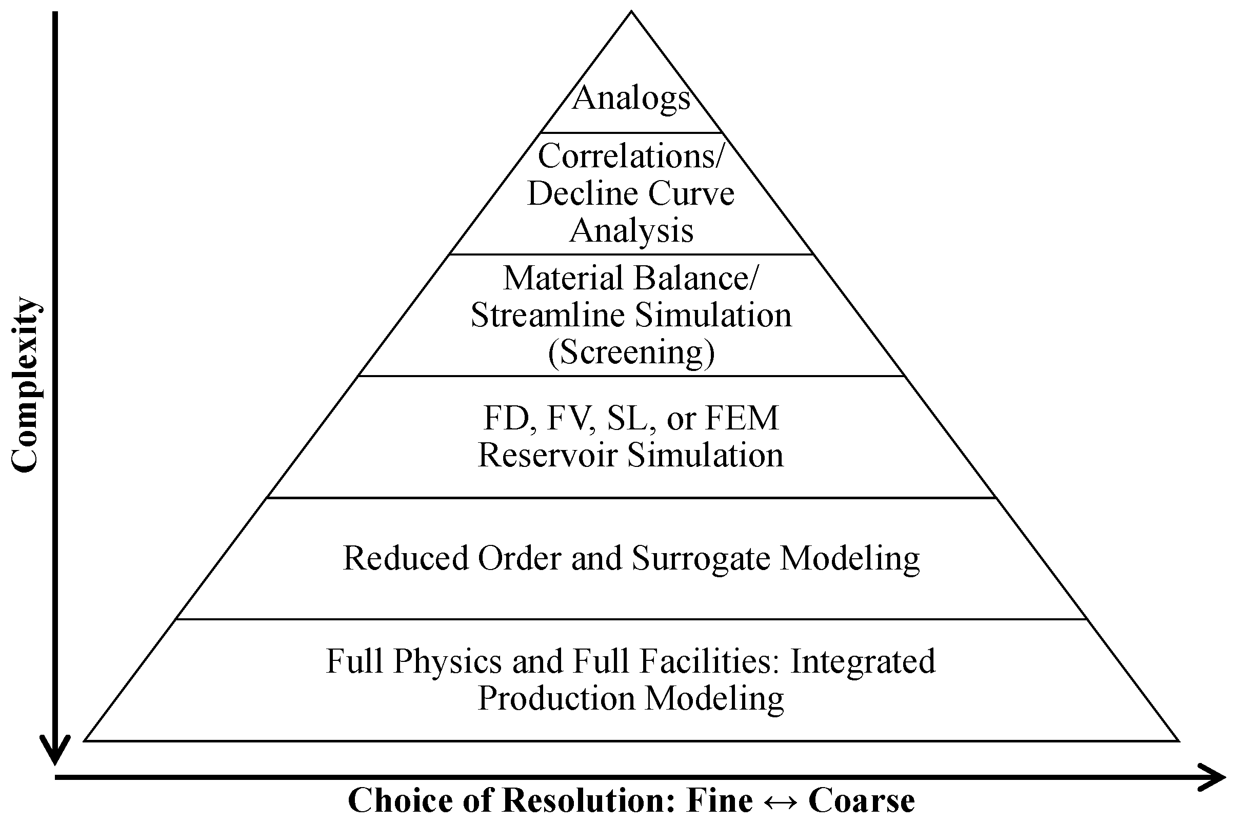
10. Other Reduced Complexity Models

As pointed out before, one of the main benefits of the CRM family of models is that it can serve as a proxy for fast and accurate simulation in field development plans. To this end, CRM can be recast into a much bigger umbrella of models, namely reduced complexity models. This comprises material balance models, reduced-physics, reduced-order models based on projection, data-driven methods, streamlines and upscaling/upgridding methodologies. It is not the intention of this section to serve as a comprehensive review of all of these technologies, as hundreds if not thousands of publications can be extracted from these topics. However, the objective here is to put the CRM into a bigger perspective of proxy modeling related to interwell connectivities.
In the context of material balance modeling, Havlena and Odeh [109,110] postulated a straight line equation to describe the production in reservoirs of different drive mechanisms, and presented field examples supporting their approach. In fact, obtaining material balance equations for reservoirs can be a relatively simple task; however, establishing a criteria that reasonable solutions should fulfill is a more complex question in reservoir engineering. Therefore, these simple models help to establish additional necessary conditions that a reasonable reservoir model should meet, mitigating the problem of non-unique parameters. Other low-order models have been applied to simulate the reservoir’s short-term production response or characterize flow units, some of them with similarities to CRM. In particular, methodologies connecting dynamical and control systems theory can lead to new insights regarding interwell connectivity.
Rowan and Clegg [21] introduced a control systems approach to reservoir engineering problems. Fox et al. [18] formulated material balance state-space equations to infer pore volumes and communication between reservoir regions under primary production. Heijn et al. [111] analyzed five methods to obtain a reduced order reservoir model, including subspace identification (black-box model) and methods for model order reduction from discretized high order reservoir models. Ershagi et al. [112] proposed a model for waterflooding production response to variations in injection rates that was based on the superposition of finite impulse responses (FIR), the input signals were decomposed on orthogonal wavelet bases to facilitate history matching. Lee et al. [113] presented applications of the FIR model and applied a least squares approach with truncated FIR order for history matching. Lee et al. [114] proposed a multi-variate autoregressive model with exogenous inputs (MARX) that was derived from material balance equations and considered producer–producer interactions and constant producers’ BHPs, where the model parameters can be estimated through linear regression. Rezapour et al. [115] presented a brief review of some low-order reservoir models and their application to waterflooding. Wang et al. [58] proposed a state-space model based on material balance equations for waterflooding in low-permeability reservoirs. Additionally, multiple analytical models based on interwell connectivity have been developed, e.g., multiwell productivity index [116,117,118], flow-network model [119], and interwell numerical simulation model [120,121].
As previously mentioned, there are many algorithms that can be used for systems identification (i.e., history matching); however, for a physics-based model, it is important to choose an algorithm capable of honoring all of the physical constraints of the system. One advantage of using a reduced-order physics-based model is that the parameters can be directly interpreted and provide insight for operational decisions. Another advantage is that the models tend to be more reliable for prediction because the functional form is derived from the underlying physical understanding of the reservoir dynamics rather than only correlations of the observed data.
To this end, projection-based model reduction methods have been used successfully in reservoir simulation and optimization. They work with the full underlying physics of the flow in porous media, and approximations are done in the context of matrices and solvers. The methodologies applied to reservoir simulation are vast, but the main algorithms in the nonlinear spectrum of models are: the proper orthogonal decomposition (POD) method [122,123], trajectory piecewise linearization (TPWL) technique [124,125], discrete empirical interpolation method (DEIM) [123,126], and quadratic-bilinear-model order reduction [127]. Many of these technologies are, indeed, part of the larger umbrella of approximation of dynamical systems, whereby the physical phenomena is recast into an input–output transfer function. Associations with interwell connectivities, as in the case of CRM, can be made through the controllability and observability properties of dynamical systems [128]. The keen reader can look at the book of Antoulas [129] for a more in depth discussion of these issues. Holanda et al. [52] combined a projection-based model reduction with CRM and demonstrated that one can obtain a hyper-reduced system of much lower order as compared with the original CRM.
Although projection-based methods are a very active research area, recently, several works have been published in the realm of data-driven methodologies to cover data mining and data analytics to assimilate the available deluge of production data being generated from unconventional and conventional reservoirs. One of the drawbacks of the reduced-order model framework is that it does not take into account real-time data to improve on the model prediction, unless some form of estimation techniques (e.g., Kalman filtering) is used [31]. Thus, the ideal framework would be to combine data and model reduction into a hybrid formulation. This, indeed, should be the “holy-grail” of any CRM-like modeling. The authors highlight three books and references therein [130,131,132], which are moving into this new direction. This is a new frontier in reservoir simulation and definitely a follow up paper devoted solely to data-driven models can be sought after this first review.

11. Unresolved Issues and Suggestions for Future Research

Despite the efforts over the last decade to widen the range of applicability of CRMs, there are still some generic limitations in these models, as in any type of model. For practical purposes, these limitations serve as indicators that help to identify situations when other modeling solutions (e.g., streamlines simulation) should be pursued from the beginning of the analyses. For research purposes, understanding and addressing these limitations can lead to new, more robust, practical models.

11.1. Gas Content of Reservoir Fluids

CRMs assume that the reservoir fluids are undersaturated and slightly compressible. For this reason, reservoirs with a gas cap, or where wells are experiencing gas coning are automatically excluded from CRM case studies. Therefore, in future works, it would be interesting to test the accuracy of the current models, and develop solutions capable of accommodating such cases.
In the cases of gas injection, the total compressibility is a function of reservoir pressure and saturation, which possibly causes significant variations in time constants (Equation (4)) and productivity indices during the history matching and forecasting windows. However, some field applications did not present a specific formulation to address this issue during gas injection [12,15,81], and still obtained satisfactory results for the analysis performed, suggesting that, in some cases, it may not be necessary to consider the time-varying behavior of the parameters. For example, in supercritical conditions, carbon dioxide behaves like a liquid [14]. Laochamroonvorapongse et al. [13] propose to segment the history matching window to capture events that are expected to cause significant variations in the parameters. This is a valid approach to analyze how the parameters are evolving with time, but it has limited predictive capability. Additionally, Nguyen [47] (Chapter 6) introduces a more complex fractional flow model for water-CO 2 flooding that incorporates relative permeability effects.
Despite the expected time-varying behavior of τ ’s and J’s, many times, the circumstances might be that producers are operated at nearly constant minimum BHP during the selected time window, which eliminates the need to estimate J, while the history matching objective function (Equation (21)) is generally less sensitive to τ ’s than to f i j ’s [31,32,33]. Under these circumstances, the time varying behavior of τ ’s and J’s might not be noticed. This is a topic that deserves attention in future research; it is necessary to perform a thorough sensitivity analysis using a set of grid-based reservoir models for validation in order to define ranges of reservoir parameters controlling the applicability of CRM to gas flooding, similar to the approach of Kaviani et al. [32] for waterflooding.

11.2. Rate Measurements

Even though the CRM equations assume that the flow rates are in reservoir conditions, frequently these values are input in surface conditions. The cause of this problem might be that flow rates are measured at the separator if a multiphase flowmeter is not incorporated in the wellheads. This issue is easy to solve if formation volume factors and average reservoir pressure estimates are available. A more complicated problem is when the flow rate measurements available are for the commingled production of some wells. In these cases, it is common to assume an allocation factor to separate the production from each well, which does not honor the reservoir dynamics. Indeed, a more robust approach would be a coupled simulator of CRM and the production system (nodal analysis).

11.3. Well-Orientation and Completion Type

Although most examples that compare CRM with grid-based reservoir models are based on fully penetrating vertical wells, this is not a model assumption. The CRMs simply assume material balance within a network structure, the fluid flow aspects related to well-orientation and completion type are not explicitly considered. Stated differently, the time constant parameter ( τ ) contains the well productivity index; therefore, the well-orientation issue does not arise explicitly. In this context, the following studies applied CRM in more specific cases:
  • horizontal wells—[133] (Chapter 4), [12] (p. 120), [91,103,134,135,136],
  • slanted wells—[133] (Chapter 4),
  • partially-penetrating wells—[79].
In fact, the well geometry plays an important role while trying to interpret interwell connectivities and establish their relationship to reservoir geology. For vertical wells, the near-well region is more influential than the interwell region on connectivity. This was used to detect wormhole development [43]. To reduce the dependency of the connectivities on the near-well geometry and rock properties, Soroush [133] proposed two approaches:
  • The reverse-CM, wherein the injection rates are history matched while the production rates serve as input variables,
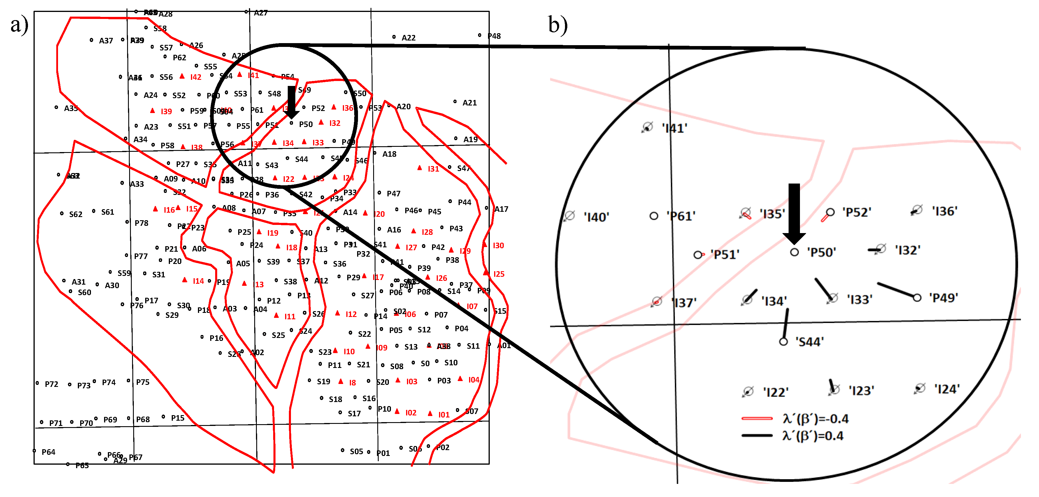
  • Subtracting the homogeneous connectivity calculated by the multiwell productivity index (MPI) approach to obtain a ‘geometry adjusted’ connectivity, as was done for Figure 11.
Soroush et al. [43] also proposed the compensated CM which allows for skin changes, which can be a cause for apparent productivity index changes. For horizontal wells, the connectivity-geology relation is more strongly related to the interwell features; this factor enabled correlation of seismic impedance to connectivity in Mirzayev et al. [134]. Therefore, as in these previous studies, it is important to consider well-orientation and completion type while analyzing the results.

11.4. Time-Varying Behavior of the CRM Parameters

In order to improve robustness of CRMs, a valid attempt is to capture and model the time varying behavior of their parameters as flooding evolves and flow patterns change. As previously discussed, some developments already have been done [30,31,76,137]; however there is not a general formulation that is well accepted yet. For example, shut-in wells remain a problem; while the compensated CM [20] is useful for more reliable interwell connectivity estimates and history matching, it is not predictive. Although generalization problems are quite challenging, this is a recommended subject for future research where theory and algorithms from pattern recognition and machine learning can be helpful. In this context, there are many avenues to be explored which might improve accuracy and account for model uncertainty. Many algorithms honor the physical aspects of the models, for example, Bayesian techniques; this is a fundamental aspect to consider before selecting algorithms.

11.5. CRM Coupling with Fractional Flow Models and Well Control Optimization

The coupling of CRM and fractional flow models assumes that interwell connectivities are equivalent to streamline allocation factors. The previous comparisons [44,47] show that there is usually a fair correlation between these two parameters; however, for some injector–producer pairs, the differences might be significant [33,134]. This impacts the oil production forecasts and optimization results. Therefore, a suggestion to future works is to develop more consistent coupling of CRM and fractional flow models in a way that is capable of identifying and correcting the well pairs that present such discrepancies.
Hong et al. [94] compared the optimization results from CRM and grid-based reservoir simulation, proposing a methodology to integrate both models, reducing computational time and checking the reliability of CRM as a proxy-model. Their results indicated that CRM provided near-optimal results for the reservoir models analyzed in their case studies. In optimization studies, this comparison with grid-based reservoir models to assess the optimality of the proposed solutions is fundamental to provide more confidence, and must become a common practice. Additionally, it may be important to have the capability of considering simultaneously primary and secondary constraints (flow rates, BHPs, and water cut) to monitor injectivity issues, fracturing pressures, gas coning and economic limits while optimizing control.

12. Conclusions

Reservoir modeling requires a balance involving flow process and geological sophistication and the purpose for which a model is developed. During the last two decades, a number of methods have been proposed to engineer practical solutions to displacement processes in fields for which data are scarce. As is typical of such methods, the CRMs have assumptions which reduce data dependence at the cost of providing simplified representations of the displacement process and reservoir complexities. Nonetheless, several versions of CRMs have been proved to be useful for many reservoir engineering applications. The following points summarize the content and findings of this review paper:
  • Several aspects must be considered in the design of CRMs to ensure that their applications are fit for purpose. For example, control volume schemes (that is, CRMT, CRMP, CRMIP, CRM-Block, ML-CRM), fractional flow models (that is, Buckley–Leverett based, semi-empirical power-law, and Koval models), optimization algorithms for the history matching and well-control optimization, dimensionality reduction techniques, and data quality and availability.
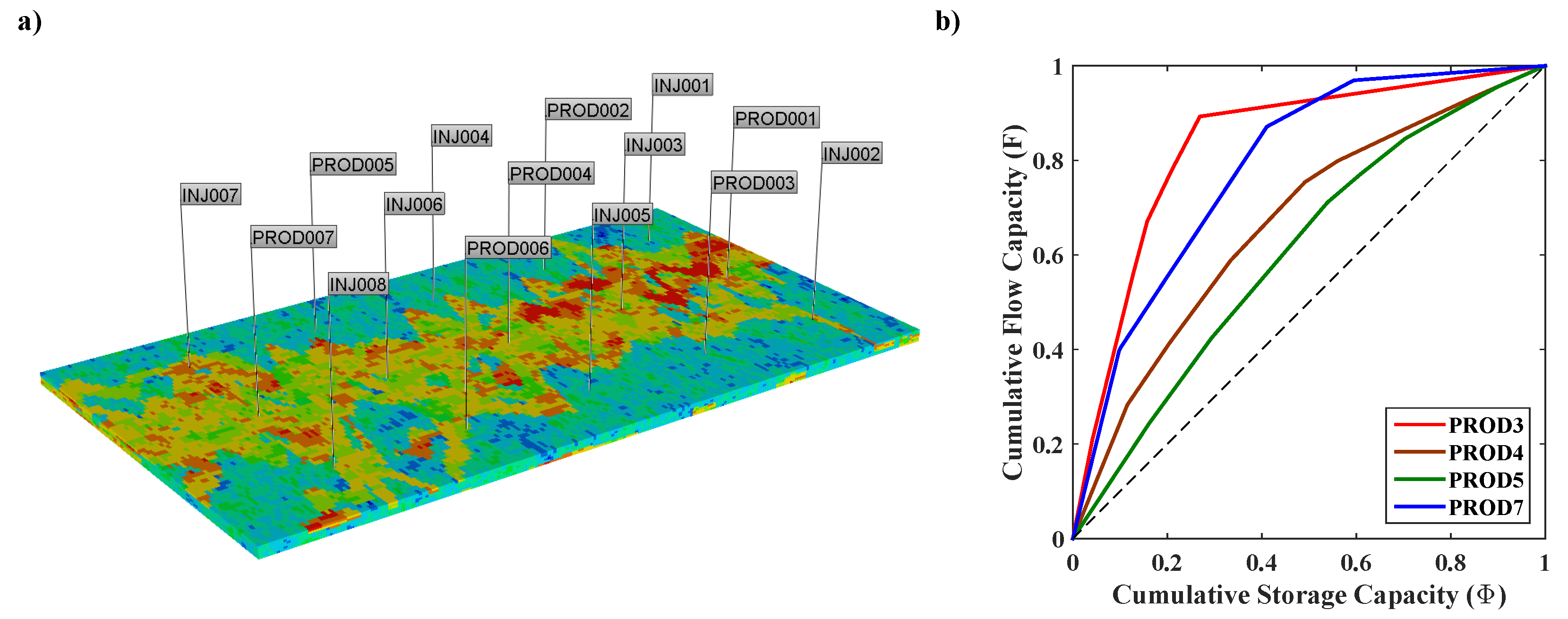
  • The physical meaning of interwell connectivities, time constants, and productivity indices are well understood. For this reason, diagnostic plots from these parameters (that is, connectivity maps, flow capacity plots, and compartmentalization plots) add value to the geological analysis, quickly providing insights into flow patterns and flood efficiencies.
  • If the model parameters are considered constant (linear time-invariant system), there is a general matrix structure and solution to all CRM control volume schemes presented in this paper.
  • Although CRMs started with mature fields undergoing waterflood, these models were extended to primary recovery, enhanced oil recovery (that is, CO 2 flooding, WAG, SWAG, polymer flooding, hot waterflooding), and prebreakthrough scenario in waterflooded fields.
  • CRMs are a fast tool for well control optimization in fields with many wells; usually, only production and injection flow rates, producers’ BHP, and well locations are required to obtain the models.
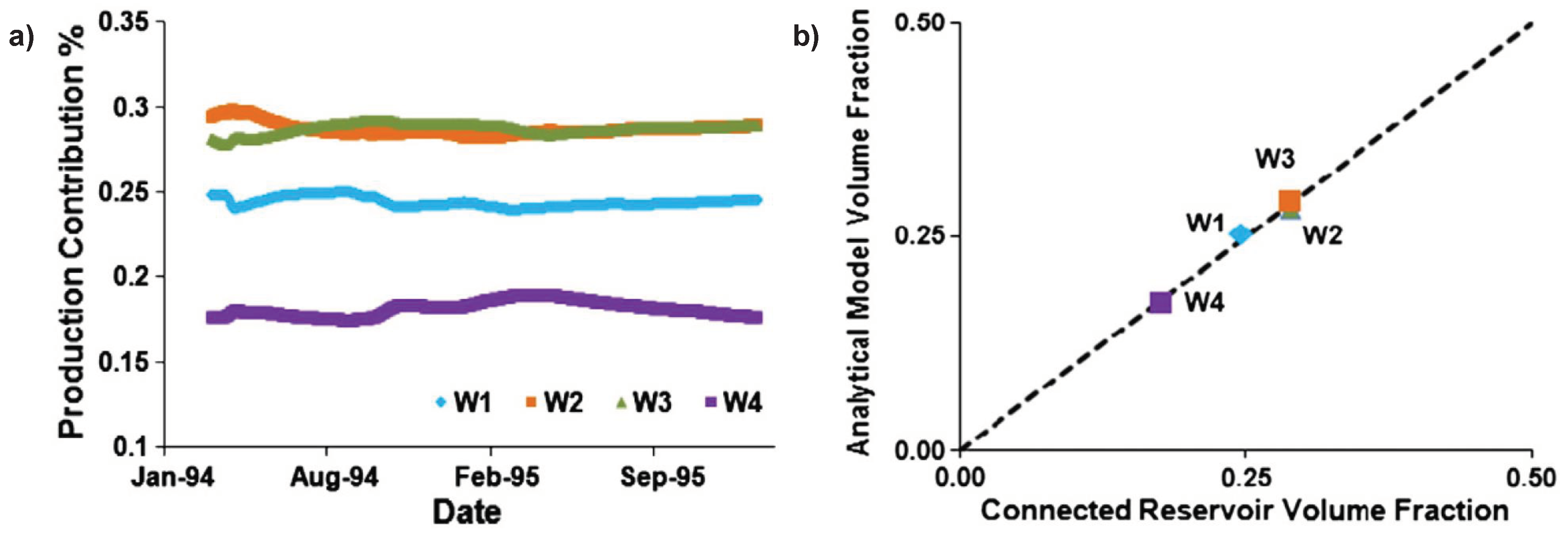
  • As an output of the CRM framework, interwell connectivity maps can assist the geological analyses by (1) corroborating results from tracer tests and 4D seismic; (2) determining main directions of flow and the presence of sealing faults, fracture swarms, and high permeability channels; and (3) delineating sand bodies. In addition, CRMs allow for quantifying the drainage volumes associated with each producer.
  • Over the last decade, CRMs have also provided valuable insights into the development of other types of reduced-physics models for reservoir simulations.
  • Naturally, there will always be room for innovative CRM developments that can provide practical solutions for improving robustness in reservoir characterization, production forecast, and optimization. Currently, the main opportunities exist in (1) improvement in production data quality; (2) understanding model limitations and modeling time-varying behaviors; and (3) more consistent coupling of CRM and fractional flow models.

Author Contributions

R.W.d.H. collected and organized the references, developed computational codes for figures illustrating concepts, and wrote Section 1, Section 2, Section 3, Section 4, Section 5, Section 6 and Section 7, Section 11 and Section 12. E.G. wrote Section 10, and obtained research funding. J.L.J. wrote Section 2 and Section 8. L.W.L. wrote Section 4. C.S.K. wrote Section 9. All authors engaged in multiple discussions regarding the content and structure of the manuscript, participated in the processes of addressing the revisions and proofreading, and suggested references.

Funding

R.W.d.H. and E.G. thank Energi Simulation (formerly Foundation CMG) for supporting this research.

Acknowledgments

The authors acknowledge the contributions of all anonymous reviewers. Figure 12, Figure 13, Figure 14, Figure 15, Figure 16 and Figure 17 are reprinted with permission. J.L.J. holds the Schulich Chair in Geostatistics at the University of Calgary. L.W.L. holds the Shahid and Sharon Ullah Chair.

Conflicts of Interest

The authors declare no conflict of interest.

Nomenclature

a linear inequality constraint matrix
Adrainage area of the control volume, ft 2
A state matrix
a eq linear equality constraint matrix
b linear inequality constraint vector
Bnumber of blocks
B input matrix
b eq linear equality constraint vector
CCRM number
C output matrix
C e error covariance matrix
c t total compressibility, psi 1
D feedforward matrix
Eeffective oil-solvent viscosity ratio
finterwell connectivity
Fcumulative flow capacity
f fraction of injected flow rate allocated to each layer
f o fractional flow of oil
f P L T fraction of production flow rate coming from each layer
f w fractional flow of water
G ( s ) transfer function
Hheterogeneity factor
I identity matrix
Jproductivity index, bbl/(day × psi)
kpermability, md
K v a l Koval factor
Lratio of sampled data points to number of parameters
l b lower bound vector
moil relative permeability exponent
Mend-point mobility ratio
nwater relative permeability exponent
N f t number of time steps until end of forecasting window
N i n j number of injectors
N L number of layers
N p cumulative liquid production, bbl
N p a r number of parameters
N p r o d number of producers
N t number of time steps until end of history matching window
N P V net present value
ppressure, psi
p ¯ average pressure of the control volume, psi
p w f or BHPproducer bottomhole pressure, psi
qliquid production rate, bbl/day
q liquid production rates vector, bbl/day
q B H P contribution of unknown BHP variations to flow rate, bbl/day
q p liquid production rate disregarding crossflow, bbl/day
Q c crossflow between layers, bbl/day
rdiscount rate per period
sLaplace variable
Snormalized average water saturation
S o r residual oil saturation
S w water saturation
S w r irreducible water saturation
ttime, day
t D dimensionless time
Ttransmissibility, bbl/(day × psi)
T s segmented time, day
u input vector
u b upper bound vector
U ( s ) input vector in Laplace space
U t well trajectories matrix for optimization
V p pore volume, bbl
winjection rate, bbl/day
w * effective water injected in the control volume, bbl/day
Wcumulative water injected, bbl
W * effective cumulative water injected in the control volume, bbl/day
x state vector
x D dimensionless distance
y output vector
Y ( s ) output vector in Laplace space
zhistory matching objective function
Greek Letters
α power-law coefficient for semi-empirical fractional flow model
β power-law exponent for semi-empirical fractional flow model
λ v j interwell connectivity between virtual injector and producer
μ viscosity, cp
ρ density, lbm/bbl
τ time constant, day
τ p time constant for primary production, day
ϕ porosity
Φ cumulative storage capacity
χ parameters vector
ω price
Subscripts and Superscripts
aaquifer
bb-th block
c a p capacity of the surface facilities
ii-th injector
i n input
jj-th producer
kk-th time step
m a x maximum
m i n minimum
ooil
obs observed data
o u t output
pred predicted data
ssolvent
vv-th producer is shut-in
wwater
α α -th layer

References

  1. Gildin, E.; King, M. Robust Reduced Complexity Modeling (R2CM) in Reservoir Engineering. In Proceedings of the Foundation CMG Summit, Calgary, AB, Canada, 24–25 June 2013. [Google Scholar]
  2. Bruce, W.A. An Electrical Device for Analyzing Oil-reservoir Behavior. Pet. Technol. 1943, 151, 112–124. [Google Scholar] [CrossRef]
  3. McCartney, S. ENIAC: The Triumphs and Tragedies of the World’s First Computer; Walker & Company: New York, NY, USA, 1999. [Google Scholar]
  4. Muskat, M. The Flow of Homogeneous Fluids Through Porous Media; Technical Report; McGraw-Hill: New York, NY, USA, 1937. [Google Scholar]
  5. Wahl, W.; Mullins, L.; Barham, R.; Bartlett, W. Matching the Performance of Saudi Arabian Oil Fields with an Electrical Model. J. Pet. Technol. 1962, 14, 1275–1282. [Google Scholar] [CrossRef]
  6. Munira, S. An Electric Circuit Network Model for Fluid Flow in Oil Reservoir. Master’s Thesis, University of Texas, Austin, TX, USA, 2010. [Google Scholar]
  7. Yousef, A.A.; Gentil, P.H.; Jensen, J.L.; Lake, L.W. A Capacitance Model to Infer Interwell Connectivity from Production and Injection Rate Fluctuations. SPE Reserv. Eval. Eng. 2006, 9, 630–646. [Google Scholar] [CrossRef]
  8. Liang, X.; Weber, D.; Edgar, T.F.; Lake, L.W.; Sayarpour, M.; Al-Yousef, A. Optimization Of Oil Production Based on A Capacitance Model of Production and Injection Rates. In Proceedings of the Hydrocarbon Economics and Evaluation Symposium, Dallas, TX, USA, 1–3 April 2007; Society of Petroleum Engineers: Richardson, TX, USA, 2007. [Google Scholar] [CrossRef]
  9. Sayarpour, M.; Zuluaga, E.; Kabir, C.S.; Lake, L.W. The use of capacitance-resistance models for rapid estimation of waterflood performance and optimization. J. Pet. Sci. Eng. 2009, 69, 227–238. [Google Scholar] [CrossRef]
  10. Nguyen, A.P.; Kim, J.S.; Lake, L.W.; Edgar, T.F.; Haynes, B. Integrated Capacitance Resistive Model for Reservoir Characterization in Primary and Secondary Recovery. In Proceedings of the SPE Annual Technical Conference and Exhibition, Denver, CO, USA, 30 October–2 November 2011; Society of Petroleum Engineers: Richardson, TX, USA, 2011. [Google Scholar] [CrossRef]
  11. Izgec, O.; Kabir, C.S. Quantifying reservoir connectivity, in-place volumes, and drainage-area pressures during primary depletion. J. Pet. Sci. Eng. 2012, 81, 7–17. [Google Scholar] [CrossRef]
  12. Sayarpour, M. Development and Application of Capacitance-Resistive Models to Water/CO2 Floods. Ph.D. Dissertation, University of Texas, Austin, TX, USA, 2008. [Google Scholar]
  13. Laochamroonvorapongse, R.; Kabir, C.; Lake, L.W. Performance assessment of miscible and immiscible water-alternating gas floods with simple tools. J. Pet. Sci. Eng. 2014, 122, 18–30. [Google Scholar] [CrossRef]
  14. Eshraghi, S.E.; Rasaei, M.R.; Zendehboudi, S. Optimization of miscible CO2 EOR and storage using heuristic methods combined with capacitance/resistance and Gentil fractional flow models. J. Natl. Gas Sci. Eng. 2016, 32, 304–318. [Google Scholar] [CrossRef]
  15. Yin, Z.; MacBeth, C.; Chassagne, R.; Vazquez, O. Evaluation of inter-well connectivity using well fluctuations and 4D seismic data. J. Pet. Sci. Eng. 2016, 145, 533–547. [Google Scholar] [CrossRef]
  16. Dake, L.P. Fundamentals of Reservoir Engineering; Elsevier: Amsterdam, The Netherlands, 1983; Volume 8. [Google Scholar]
  17. Yousef, A.A. Investigating Statistical Techniques to Infer Interwell Connectivity from Production and Injection Rate Fluctuations. Ph.D. Dissertation, University of Texas, Austin, TX, USA, 2006. [Google Scholar]
  18. Fox, M.J.; Chedburn, A.C.S.; Stewart, G. Simple Characterization of Communication between Reservoir Regions. In Proceedings of the European Petroleum Conference, London, UK, 16–19 October 1988; Society of Petroleum Engineers: Richardson, TX, USA. [Google Scholar] [CrossRef]
  19. Weber, D. The Use of Capacitance-Resistance Models to Optimize Injection Allocation and Well Location in Water Floods. Ph.D. Dissertation, University of Texas, Austin, TX, USA, 2009. [Google Scholar]
  20. Kaviani, D.; Jensen, J.L.; Lake, L.W. Estimation of interwell connectivity in the case of unmeasured fluctuating bottomhole pressures. J. Pet. Sci. Eng. 2012, 90–91, 79–95. [Google Scholar] [CrossRef]
  21. Rowan, G.; Clegg, M. The Cybernetic Approach To Reservoir Engineering. In Proceedings of the Fall Meeting of the Society of Petroleum Engineers of AIME, New Orleans, LA, USA, 6–9 October 1963; Society of Petroleum Engineers: Richardson, TX, USA, 1963. [Google Scholar] [CrossRef]
  22. Seborg, D.E.; Mellichamp, D.A.; Edgar, T.F.; Doyle, F.J., III. Process Dynamics and Control, 3rd ed.; John Wiley & Sons: Hoboken, NJ, USA, 2011. [Google Scholar]
  23. Kaviani, D.; Valkó, P.P.; Jensen, J.L. Application of the Multiwell Productivity Index-Based Method to Evaluate Interwell Connectivity. In Proceedings of the SPE Improved Oil Recovery Symposium, Tulsa, OK, USA, 24–28 April 2010; Society of Petroleum Engineers: Richardson, TX, USA, 2010. [Google Scholar] [CrossRef]
  24. Liang, X. A simple model to infer interwell connectivity only from well-rate fluctuations in waterfloods. J. Pet. Sci. Eng. 2010, 70, 35–43. [Google Scholar] [CrossRef]
  25. Holanda, R.W.D. Capacitance Resistance Model in a Control Systems Framework: A Tool for Describing and Controlling Waterflooding Reservoirs. Master’s Thesis, Texas A&M University, College Station, TX, USA, 2015. [Google Scholar]
  26. Sayyafzadeh, M.; Pourafshary, P.; Haghighi, M.; Rashidi, F. Application of transfer functions to model water injection in hydrocarbon reservoir. J. Pet. Sci. Eng. 2011, 78, 139–148. [Google Scholar] [CrossRef]
  27. Kabir, C.S.; Lake, L.W. A Semianalytical Approach to Estimating EUR in Unconventional Reservoirs. In Proceedings of the North American Unconventional Gas Conference and Exhibition, The Woodlands, TX, USA, 14–16 June 2011; Society of Petroleum Engineers: Richardson, TX, USA, 2011. [Google Scholar] [CrossRef]
  28. Li, Y.; Júlíusson, E.; Pálsson, H.; Stefánsson, H.; Valfells, A. Machine learning for creation of generalized lumped parameter tank models of low temperature geothermal reservoir systems. Geothermics 2017, 70, 62–84. [Google Scholar] [CrossRef]
  29. Mamghaderi, A.; Bastami, A.; Pourafshary, P. Optimization of waterflooding performance in a layered reservoir using a combination of capacitance-resistive model and genetic algorithm method. J. Energy Resour. Technol. 2012, 135, 013102. [Google Scholar] [CrossRef]
  30. Moreno, G.A. Multilayer capacitance-resistance model with dynamic connectivities. J. Pet. Sci. Eng. 2013, 109, 298–307. [Google Scholar] [CrossRef]
  31. Jafroodi, N.; Zhang, D. New method for reservoir characterization and optimization using CRM-EnOpt approach. J. Pet. Sci. Eng. 2011, 77, 155–171. [Google Scholar] [CrossRef]
  32. Kaviani, D.; Soroush, M.; Jensen, J.L. How accurate are capacitance model connectivity estimates? J. Pet. Sci. Eng. 2014, 122, 439–452. [Google Scholar] [CrossRef]
  33. Holanda, R.W.D.; Gildin, E.; Jensen, J.L. A generalized framework for Capacitance Resistance Models and a comparison with streamline allocation factors. J. Pet. Sci. Eng. 2018, 162, 260–282. [Google Scholar] [CrossRef]
  34. Mamghaderi, A.; Pourafshary, P. Water flooding performance prediction in layered reservoirs using improved capacitance-resistive model. J. Pet. Sci. Eng. 2013, 108, 107–117. [Google Scholar] [CrossRef]
  35. Zhang, Z.; Li, H.; Zhang, D. Water flooding performance prediction by multi-layer capacitance-resistive models combined with the ensemble Kalman filter. J. Pet. Sci. Eng. 2015, 127, 1–19. [Google Scholar] [CrossRef]
  36. Fraguío, M.; Lacivita, A.; Valle, J.; Marzano, M.; Storti, M. Integrating a Data Driven Model into a Multilayer Pattern Waterflood Simulator. In Proceedings of the SPE Latin America and Caribbean Mature Fields Symposium, Bahia, Brazil, 15–16 March 2017; Society of Petroleum Engineers: Richardson, TX, USA, 2017. [Google Scholar] [CrossRef]
  37. Gamarra, F.C.; Ramos, N.E.; Borsani, I. Estimation of Mature Water Flooding Performance in EOR by Using Capacitance Resistive Model and Fractional Flow Model by Layer. 2017. Available online: https://www.researchgate.net/publication/317585961_Estimation_of_Mature_Water_Flooding_Performance _in_EOR_by_Using_Capacitance_Resistive_Model_and_Fractional_Flow_model_by_layer (accessed on 28 November 2018).
  38. Zhang, Z.; Li, H.; Zhang, D. Reservoir characterization and production optimization using the ensemble-based optimization method and multi-layer capacitance-resistive models. J. Pet. Sci. Eng. 2017, 156, 633–653. [Google Scholar] [CrossRef]
  39. Prakasa, B.; Shi, X.; Muradov, K.; Davies, D. Novel Application of Capacitance-Resistance Model for Reservoir Characterisation and Zonal, Intelligent Well Control. In Proceedings of the SPE/IATMI Asia Pacific Oil & Gas Conference and Exhibition, Jakarta, Indonesia, 17–19 October 2017; Society of Petroleum Engineers: Richardson, TX, USA, 2017. [Google Scholar] [CrossRef]
  40. Albertoni, A.; Lake, L.W. Inferring interwell connectivity only from well-rate fluctuations in waterfloods. SPE Reserv. Eval. Eng. 2003, 6, 6–16. [Google Scholar] [CrossRef]
  41. Dinh, A.; Tiab, D. Inferring interwell connectivity from well bottomhole-pressure fluctuations in waterfloods. SPE Reserv. Eval. Eng. 2008, 11, 874–881. [Google Scholar] [CrossRef]
  42. Gentil, P.H. The Use of Multilinear Regression Models in Patterned Waterfloods: Physical Meaning of the Regression Coefficients. Master’s Thesis, University of Texas, Austin, TX, USA, 2005. [Google Scholar]
  43. Soroush, M.; Kaviani, D.; Jensen, J.L. Interwell connectivity evaluation in cases of changing skin and frequent production interruptions. J. Pet. Sci. Eng. 2014, 122, 616–630. [Google Scholar] [CrossRef]
  44. Izgec, O.; Kabir, C. Understanding reservoir connectivity in waterfloods before breakthrough. J. Pet. Sci. Eng. 2010, 75, 1–12. [Google Scholar] [CrossRef]
  45. Izgec, O.; Kabir, C.S. Quantifying nonuniform aquifer strength at individual wells. SPE Reserv. Eval. Eng. 2010, 13, 296–305. [Google Scholar] [CrossRef]
  46. Izgec, O. Understanding waterflood performance with modern analytical techniques. J. Pet. Sci. Eng. 2012, 81, 100–111. [Google Scholar] [CrossRef]
  47. Nguyen, A.P. Capacitance Resistance Modeling for Primary Recovery, Waterflood and Water-CO2 Flood. Ph.D. Dissertation, University of Texas, Austin, TX, USA, 2012. [Google Scholar]
  48. Mirzayev, M.; Riazi, N.; Cronkwright, D.; Jensen, J.L.; Pedersen, P.K. Determining Well-to-Well Connectivity in Tight Reservoirs. In Proceedings of the SPE/CSUR Unconventional Resources Conference, Calgary, AB, Canada, 20–22 October 2015; Society of Petroleum Engineers: Richardson, TX, USA, 2015. [Google Scholar] [CrossRef]
  49. Parekh, B.; Kabir, C. A case study of improved understanding of reservoir connectivity in an evolving waterflood with surveillance data. J. Pet. Sci. Eng. 2013, 102, 1–9. [Google Scholar] [CrossRef]
  50. Thiele, M.R.; Batycky, R.P. Using streamline-derived injection efficiencies for improved waterflood management. SPE Reserv. Eval. Eng. 2006, 9, 187–196. [Google Scholar] [CrossRef]
  51. Economides, M.; Hill, A.; Ehlig-Economides, C.; Zhu, D. Petroleum Production Systems, 2nd ed.; Prentice Hall: Upper Saddle River, NJ, USA, 2013. [Google Scholar]
  52. Holanda, R.W.D.; Gildin, E.; Jensen, J.L. Improved Waterflood Analysis Using the Capacitance-Resistance Model Within a Control Systems Framework. In Proceedings of the SPE Latin American and Caribbean Petroleum Engineering Conference, Quito, Ecuador, 18–20 November 2015; Society of Petroleum Engineers: Richardson, TX, USA, 2015. [Google Scholar] [CrossRef]
  53. Holanda, R.W.D.; Gildin, E.; Valkó, P.P. Combining physics, statistics, and heuristics in the decline-curve analysis of large data sets in unconventional reservoirs. SPE Reserv. Eval. Eng. 2018. [Google Scholar] [CrossRef]
  54. Oliver, D.S.; Reynolds, A.C.; Liu, N. Inverse Theory for Petroleum Reservoir Characterization and History Matching; Cambridge University Press: Cambridge, UK, 2008. [Google Scholar]
  55. Oliver, D.S.; Chen, Y. Recent progress on reservoir history matching: A review. Comput. Geosci. 2011, 15, 185–221. [Google Scholar] [CrossRef]
  56. Kang, Z.; Zhao, H.; Zhang, H.; Zhang, Y.; Li, Y.; Sun, H. Research on applied mechanics with reservoir interwell dynamic connectivity model and inversion method in case of shut-in wells. Appl. Mech. Mater. 2014, 540, 296–301. [Google Scholar] [CrossRef]
  57. Lasdon, L.; Shirzadi, S.; Ziegel, E. Implementing CRM models for improved oil recovery in large oil fields. Optim. Eng. 2017, 18, 87–103. [Google Scholar] [CrossRef]
  58. Wang, D.; Niu, D.; Li, H.A. Predicting waterflooding performance in low-permeability reservoirs with linear dynamical systems. SPE J. 2017, 22, 1596–1608. [Google Scholar] [CrossRef]
  59. Sayarpour, M.; Kabir, C.; Sepehrnoori, K.; Lake, L.W. Probabilistic history matching with the capacitance-resistance model in waterfloods: A precursor to numerical modeling. J. Pet. Sci. Eng. 2011, 78, 96–108. [Google Scholar] [CrossRef]
  60. Altaheini, S.; Al-Towijri, A.; Ertekin, T. Introducing a New Capacitance-Resistance Model and Solutions to Current Modeling Limitations. In Proceedings of the SPE Annual Technical Conference and Exhibition, Dubai, UAE, 26–28 September 2016; Society of Petroleum Engineers: Richardson, TX, USA, 2016. [Google Scholar] [CrossRef]
  61. Kim, J.S. Development of Linear Capacitance-Resistance Models for Characterizing Waterflooded Reservoirs. Master’s Thesis, University of Texas, Austin, TX, USA, 2011. [Google Scholar]
  62. Kim, J.S.; Lake, L.W.; Edgar, T.F. Integrated Capacitance-Resistance Model for Characterizing Waterflooded Reservoirs. In Proceedings of the IFAC Workshop on Automatic Control in Offshore Oil and Gas Production, Trondheim, Norway, 31 May–1 June 2012; International Federation of Automatic Control: Laxenburg, Austria, 2012. [Google Scholar] [CrossRef]
  63. Kaviani, D.; Jensen, J.L. Reliable Connectivity Evaluation in Conventional and Heavy Oil Reservoirs: A Case Study from Senlac Heavy Oil Pool, Western Saskatchewan. In Proceedings of the Canadian Unconventional Resources and International Petroleum Conference, Calgary, AB, Canada, 19–21 October 2010; Society of Petroleum Engineers: Richardson, TX, USA, 2010. [Google Scholar] [CrossRef]
  64. Kaviani, D. Interwell Connectivity Evaluation from Wellrate Fluctuations: A Waterflooding Management Tool. Ph.D. Dissertation, Texas A&M University, College Station, TX, USA, 2009. [Google Scholar]
  65. Tafti, T.A.; Ershaghi, I.; Rezapour, A.; Ortega, A. Injection Scheduling Design for Reduced Order Waterflood Modeling. In Proceedings of the SPE Western Regional & AAPG Pacific Section Meeting, Monterey, CA, USA, 19–25 April 2013; Society of Petroleum Engineers: Richardson, TX, USA, 2013. [Google Scholar] [CrossRef]
  66. Moreno, G.A.; Lake, L.W. Input signal design to estimate interwell connectivities in mature fields from the capacitance-resistance model. Pet. Sci. 2014, 11, 563–568. [Google Scholar] [CrossRef]
  67. Zandvliet, M.; Bosgra, O.; Jansen, J.; den Hof, P.V.; Kraaijevanger, J. Bang-bang control and singular arcs in reservoir flooding. J. Pet. Sci. Eng. 2007, 58, 186–200. [Google Scholar] [CrossRef]
  68. Moreno, G.A.; Lake, L.W. On the uncertainty of interwell connectivity estimations from the capacitance-resistance model. Pet. Sci. 2014, 11, 265–271. [Google Scholar] [CrossRef]
  69. Cao, F. A New Method of Data Quality Control in Production Data Using the Capacitance-Resistance Model. Master’s Thesis, University of Texas, Austin, TX, USA, 2011. [Google Scholar]
  70. Buckley, S.E.; Leverett, M. Mechanism of fluid displacement in sands. Trans. AIME 1942, 146, 107–116. [Google Scholar] [CrossRef]
  71. Brooks, R.; Corey, T. Hydraulic Properties of Porous Media; Hydrology Papers; Colorado State University: Fort Collins, CO, USA, 1964. [Google Scholar]
  72. Willhite, G.P. Waterflooding; Society of Petroleum Engineers: Richardson, TX, USA, 1986. [Google Scholar]
  73. Yortsos, Y.; Choi, Y.; Yang, Z.; Shah, P. Analysis and interpretation of water/oil ratio in waterfloods. SPE J. 1999, 4, 413–424. [Google Scholar] [CrossRef]
  74. Koval, E. A method for predicting the performance of unstable miscible displacement in heterogeneous media. SPE J. 1963, 3, 145–154. [Google Scholar] [CrossRef]
  75. Cao, F. Development of a Two-Phase Flow Coupled Capacitance Resistance Model. Ph.D. Dissertation, University of Texas, Austin, TX, USA, 2014. [Google Scholar]
  76. Cao, F.; Luo, H.; Lake, L.W. Development of a Fully Coupled Two-phase Flow Based Capacitance Resistance Model (CRM). In Proceedings of the SPE Improved Oil Recovery Symposium, Tulsa, OK, USA, 12–16 April 2014; Society of Petroleum Engineers: Richardson, TX, USA, 2014. [Google Scholar] [CrossRef]
  77. Cao, F.; Luo, H.; Lake, L.W. Oil-rate forecast by inferring fractional-flow models from field data with Koval method combined with the capacitance/resistance model. SPE Reserv. Eval. Eng. 2015, 18, 534–553. [Google Scholar] [CrossRef]
  78. Lake, L.W.; Johns, R.T.; Rossen, W.R.; Pope, G.A. Fundamentals of Enhanced Oil Recovery; Society of Petroleum Engineers: Richardson, TX, USA, 2014. [Google Scholar]
  79. Yousef, A.A.; Jensen, J.L.; Lake, L.W. Integrated interpretation of interwell connectivity using injection and production fluctuations. Math. Geosci. 2009, 41, 81–102. [Google Scholar] [CrossRef]
  80. Laochamroonvorapongse, R. Advances in the Development and Application of a Capacitance-Resistance Model. Master’s Thesis, University of Texas, Austin, TX, USA, 2013. [Google Scholar]
  81. Salazar, M.; Gonzalez, H.; Matringe, S.; Castiñeira, D. Combining Decline-Curve Analysis and Capacitance-Resistance Models To Understand and Predict the Behavior of a Mature Naturally Fractured Carbonate Reservoir Under Gas Injection. In Proceedings of the SPE Latin America and Caribbean Petroleum Engineering Conference, Mexico City, Mexico, 16–18 April 2012; Society of Petroleum Engineers: Richardson, TX, USA, 2012. [Google Scholar] [CrossRef]
  82. Mollaei, A.; Delshad, M. General Isothermal Enhanced Oil Recovery and Waterflood Forecasting Model. In Proceedings of the SPE Annual Technical Conference and Exhibition, Denver, CO, USA, 30 October–2 November 2011; Society of Petroleum Engineers: Richardson, TX, USA, 2011. [Google Scholar] [CrossRef]
  83. Duribe, V.C. Capacitance Resistance Modeling for Improved Characterization in Waterflooding and Thermal Recovery Projects. Ph.D. Dissertation, University of Texas, Austin, TX, USA, 2016. [Google Scholar]
  84. Tao, Q. Modeling CO2 Leakage from Geological Storage Formation and Reducing the Associated Risk. Ph.D. Dissertation, University of Texas, Austin, TX, USA, 2012. [Google Scholar]
  85. Tao, Q.; Bryant, S.L. Optimizing CO2 storage in a deep saline aquifer with the capacitance-resistance model. Energy Procedia 2013, 37, 3919–3926. [Google Scholar] [CrossRef]
  86. Tao, Q.; Bryant, S.L. Optimizing carbon sequestration with the capacitance/resistance model. SPE J. 2015, 20, 1094–1102. [Google Scholar] [CrossRef]
  87. Akin, S. Optimization of Reinjection Allocation in Geothermal Fields Using Capacitance-Resistance Models. In Proceedings of the Thirty-Ninth Workshop on Geothermal Reservoir Engineering, Stanford, CA, USA, 24–26 February 2014. [Google Scholar]
  88. Wang, W.; Patzek, T.W.; Lake, L.W. A Capacitance-Resistive Model and InSAR Imagery of Surface Subsidence Explain Performance of a Waterflood Project at Lost Hills. In Proceedings of the SPE Annual Technical Conference and Exhibition, Denver, CO, USA, 30 October–2 November 2011; Society of Petroleum Engineers: Richardson, TX, USA, 2011. [Google Scholar] [CrossRef]
  89. Wang, W. Reservoir Characterization Using a Capacitance Resistance Model in Conjunction with Geomechanical Surface Subsidence Models. Master’s Thesis, University of Texas, Austin, TX, USA, 2011. [Google Scholar]
  90. Al-Mudhafer, W.J. Parallel Estimation of Surface Subsidence and Updated Reservoir Characteristics by Coupling of Geomechanical & Fluid Flow Modeling. In Proceedings of the North Africa Technical Conference and Exhibition, Cairo, Egypt, 15–17 April 2013; Society of Petroleum Engineers:: Richardson, TX, USA, 2013. [Google Scholar] [CrossRef]
  91. Almarri, M.; Prakasa, B.; Muradov, K.; Davies, D. Identification and Characterization of Thermally Induced Fractures Using Modern Analytical Techniques. In Proceedings of the SPE Kingdom of Saudi Arabia Annual Technical Symposium and Exhibition, Dammam, Saudi Arabia, 24–27 April 2017; Society of Petroleum Engineers: Richardson, TX, USA, 2017. [Google Scholar] [CrossRef]
  92. Weber, D.; Edgar, T.F.; Lake, L.W.; Lasdon, L.S.; Kawas, S.; Sayarpour, M. Improvements in Capacitance-Resistive Modeling and Optimization of Large Scale Reservoirs. In Proceedings of the SPE Western Regional Meeting, San Jose, CA, USA, 24–26 March 2009; Society of Petroleum Engineers: Richardson, TX, USA, 2009. [Google Scholar] [CrossRef]
  93. Stensgaard, A.D.D. Estimating the Value of Information Using Closed Loop Reservoir Management of Capacitance Resistive Models. Master’s Thesis, Norwegian University of Science and Technology, Trondheim, Norway, 2016. [Google Scholar]
  94. Hong, A.J.; Bratvold, R.B.; Nævdal, G. Robust production optimization with capacitance-resistance model as precursor. Comput. Geosci. 2017. [Google Scholar] [CrossRef]
  95. Sorek, N.; Gildin, E.; Boukouvala, F.; Beykal, B.; Floudas, C.A. Dimensionality reduction for production optimization using polynomial approximations. Comput. Geosci. 2017, 21, 247–266. [Google Scholar] [CrossRef]
  96. Sorek, N.; Zalavadia, H.; Gildin, E. Model Order Reduction and Control Polynomial Approximation for Well-Control Production Optimization. In Proceedings of the SPE Reservoir Simulation Conference, Montgomery, TX, USA, 20–22 February 2017. [Google Scholar] [CrossRef]
  97. Chitsiripanich, S. Field Application of Capacitance-Resistance Models to Identify Potential Location for Infill Drilling. Master’s Thesis, University of Texas, Austin, TX, USA, 2015. [Google Scholar]
  98. Van Essen, G.; Van den Hof, P.; Jansen, J.D. A two-level strategy to realize life-cycle production optimization in an operational setting. SPE J. 2013, 18, 1057–1066. [Google Scholar] [CrossRef]
  99. Sayarpour, M.; Kabir, C.S.; Lake, L.W. Field applications of capacitance-resistive models in waterfloods. SPE J. 2009, 12, 853–864. [Google Scholar] [CrossRef]
  100. Naudomsup, N.; Lake, L.W. Extension of Capacitance-Resistance Model to Tracer Flow for Determining Reservoir Properties. In Proceedings of the SPE Annual Technical Conference and Exhibition, San Antonio, TX, USA, 9–11 October 2017; Society of Petroleum Engineers: Richardson, TX, USA, 2017. [Google Scholar] [CrossRef]
  101. Gardner, M.H.; Dharmasamadhi, W.; Willis, B.J.; Dutton, S.P.; Fang, Q.; Kattah, S.; Yeh, J.; Wang, W. Reservoir characterization of Buck Draw Field. In Proceedings of the Bureau of Economic Geology Deltas Industrial Associates Field Trip, Rapid City, SD, USA, 9–14 October 1994. [Google Scholar]
  102. Dutton, S.P.; Willis, B.J. Comparison of outcrop and subsurface sandstone permeability distribution, Lower Cretaceous Fall River Formation, South Dakota and Wyoming. J. Sediment. Res. 1998, 68. [Google Scholar] [CrossRef]
  103. Olsen, C.; Kabir, C. Waterflood performance evaluation in a chalk reservoir with an ensemble of tools. J. Pet. Sci. Eng. 2014, 124, 60–71. [Google Scholar] [CrossRef]
  104. Jahangiri, H.R.; Adler, C.; Shirzadi, S.; Bailey, R.; Ziegel, E.; Chesher, J.; White, M. A Data-Driven Approach Enhances Conventional Reservoir Surveillance Methods for Waterflood Performance Management in the North Sea. In Proceedings of the SPE Reservoir Simulation Symposium, Utrecht, The Netherlands, 1–3 April 2014; Society of Petroleum Engineers: Richardson, TX, USA, 2014. [Google Scholar] [CrossRef]
  105. O’Reilly, D.I.; Hunt, A.J.; Sze, E.S.; Hopcroft, B.S.; Goff, B.H. Increasing Water Injection Efficiency in the Mature Windalia Oil Field, NW Australia, Through Improved Reservoir Surveillance and Operations. In Proceedings of the SPE Asia Pacific Oil & Gas Conference and Exhibition, Perth, Australia, 25–27 October 2016; Society of Petroleum Engineers: Richardson, TX, USA, 2016. [Google Scholar] [CrossRef]
  106. Jati, N.; Sayarpour, M. Capacitance Resistance Model (CRM) and Production Attribute Mapping (PAM) Integration Work Flow for Water Flood Performance Evaluation in Bravo Field. In Proceedings of the Fortieth Annual Convention & Exhibition, Jakarta, Indonesia, 25–27 May 2016; Indonesian Petroleum Association: South Jakarta, Indonesia, 2016. [Google Scholar]
  107. Nguyen, A.P.; Lasdon, L.S.; Lake, L.W.; Edgar, T.F. Capacitance Resistive Model Application to Optimize Waterflood in a West Texas Field. In Proceedings of the SPE Annual Technical Conference and Exhibition, Denver, CO, USA, 30 October–2 November 2011; Society of Petroleum Engineers: Richardson, TX, USA, 2011. [Google Scholar] [CrossRef]
  108. Al Saidi, A.; Al Wadhani, M. Application of Fast Reservoir Simulation Methods to Optimize Production by Reallocation of Water Injection Rates in an Omani Field. In Proceedings of the SPE Middle East Oil & Gas Show and Conference, Manama, Bahrain, 8–11 March 2015; Society of Petroleum Engineers: Richardson, TX, USA, 2015. [Google Scholar] [CrossRef]
  109. Havlena, D.; Odeh, A. The material balance as an equation of a straight line. J. Pet. Technol. 1963, 15, 896–900. [Google Scholar] [CrossRef]
  110. Havlena, D.; Odeh, A. The material balance as an equation of a straight line—Part II, field cases. J. Pet. Technol. 1964, 16, 815–822. [Google Scholar] [CrossRef]
  111. Heijn, T.; Markovinovic, R.; Jansen, J. Generation of low-order reservoir models using system-theoretical concepts. SPE J. 2004, 9, 202–218. [Google Scholar] [CrossRef]
  112. Ershaghi, I.; Ortega, A.; Lee, K.H.; Ghareloo, A. A Method for Characterization of Flow Units Between Injection-Production Wells Using Performance Data. In Proceedings of the SPE Western Regional and Pacific Section AAPG Joint Meeting, Bakersfield, CA, USA, 29 March–4 April 2008; Society of Petroleum Engineers: Richardson, TX, USA, 2008. [Google Scholar] [CrossRef]
  113. Lee, K.H.; Ortega, A.; Nejad, A.M.; Jafroodi, N.; Ershaghi, I. A Novel Method for Mapping Fractures and High-Permeability Channels in Waterfloods Using Injection and Production Rates. In Proceedings of the SPE Western Regional Meeting, San Jose, CA, USA, 24–26 March 2009; Society of Petroleum Engineers: Richardson, TX, USA, 2009. [Google Scholar] [CrossRef]
  114. Lee, K.H.; Ortega, A.; Jafroodi, N.; Ershaghi, I. A Multivariate Autoregressive Model for Characterizing Producer-producer Relationships in Waterfloods from Injection/Production Rate Fluctuations. In Proceedings of the SPE Western Regional Meeting, Anaheim, CA, USA, 27–29 May 2010; Society of Petroleum Engineers: Richardson, TX, USA, 2010. [Google Scholar] [CrossRef]
  115. Rezapour, A.; Ortega, A.; Ershaghi, I. Reservoir Waterflooding System Identification and Model Validation with Injection/Production Rate Fluctuations. In Proceedings of the SPE Western Regional Meeting, Garden Grove, CA, USA, 27–30 April 2015; Society of Petroleum Engineers: Richardson, TX, USA, 2015. [Google Scholar] [CrossRef]
  116. Valkó, P.P.; Doublet, L.E.; Blasingame, T.A. Development and application of the multiwell productivity index (MPI). SPE J. 2000, 5, 21–31. [Google Scholar] [CrossRef]
  117. Kaviani, D.; Valkó, P.P. Inferring interwell connectivity using multiwell productivity index (MPI). J. Pet. Sci. Eng. 2010, 73, 48–58. [Google Scholar] [CrossRef]
  118. Kaviani, D.; Valkó, P.; Jensen, J. Analysis of injection and production data for open and large reservoirs. Energies 2011, 4, 1950–1972. [Google Scholar] [CrossRef]
  119. Lerlertpakdee, P.; Jafarpour, B.; Gildin, E. Efficient production optimization with flow-network models. SPE J. 2014, 19, 1083–1095. [Google Scholar] [CrossRef]
  120. Zhao, H.; Kang, Z.; Zhang, X.; Sun, H.; Cao, L.; Reynolds, A.C. A physics-based data-driven numerical model for reservoir history matching and prediction with a field application. SPE J. 2016, 21, 2175–2194. [Google Scholar] [CrossRef]
  121. Guo, Z.; Reynolds, A.C.; Zhao, H. Waterflooding optimization with the INSIM-FT data-driven model. Comput. Geosci. 2018. [Google Scholar] [CrossRef]
  122. Jansen, J.D.; Durlofsky, L.J. Use of reduced-order models in well control optimization. Optim. Eng. 2017, 18, 105–132. [Google Scholar] [CrossRef]
  123. Yang, Y.; Ghasemi, M.; Gildin, E.; Efendiev, Y.; Calo, V. Fast multiscale reservoir simulations with POD-DEIM model reduction. SPE J. 2016, 21, 2141–2154. [Google Scholar] [CrossRef]
  124. Cardoso, M.; Durlofsky, L. Linearized reduced-order models for subsurface flow simulation. J. Comput. Phys. 2010, 229, 681–700. [Google Scholar] [CrossRef]
  125. Trehan, S.; Durlofsky, L.J. Trajectory piecewise quadratic reduced-order model for subsurface flow, with application to PDE-constrained optimization. J. Comput. Phys. 2016, 326, 446–473. [Google Scholar] [CrossRef]
  126. Tan, X.; Gildin, E.; Trehan, S.; Yang, Y.; Hoda, N. Trajectory-Based DEIM (TDEIM) Model Reduction Applied to Reservoir Simulation. In Proceedings of the SPE Reservoir Simulation Conference, Montgomery, TX, USA, 20–22 February 2017. [Google Scholar] [CrossRef]
  127. Ghasemi, M.; Gildin, E. Model order reduction in porous media flow simulation using quadratic bilinear formulation. Comput. Geosci. 2016, 20, 723–735. [Google Scholar] [CrossRef]
  128. Van Doren, J.F.M.; Van den Hof, P.M.J.; Bosgra, O.H.; Jansen, J.D. Controllability and observability in two-phase porous media flow. Comput. Geosci. 2013, 17, 773–788. [Google Scholar] [CrossRef] [Green Version]
  129. Antoulas, A.C. Approximation of Large-Scale Dynamical Systems; Society for Industrial and Applied Mathematics: Philadelphia, PA, USA, 2005; Volume 6. [Google Scholar]
  130. Mohaghegh, S.D. Data-Driven Reservoir Modeling; Society of Petroleum Engineers: Richardson, TX, USA, 2017. [Google Scholar]
  131. Mohaghegh, S.D. Shale Analytics: Data-Driven Analytics in Unconventional Resources; Springer: Berlin, Germany, 2017. [Google Scholar]
  132. Mishra, S.; Datta-Gupta, A. Applied Statistical Modeling and Data Analytics: A Practical Guide for the Petroleum Geosciences; Elsevier: Amsterdam, The Netherlands, 2017. [Google Scholar]
  133. Soroush, M. Interwell Connectivity Evaluation Using Injection and Production Fluctuation Data. Ph.D. Dissertation, University of Calgary, Calgary, AB, Canada, 2013. [Google Scholar]
  134. Mirzayev, M.; Riazi, N.; Cronkwright, D.; Jensen, J.L.; Pedersen, P.K. Determining well-to-well connectivity using a modified capacitance model, seismic, and geology for a Bakken Waterflood. J. Pet. Sci. Eng. 2017, 152, 611–627. [Google Scholar] [CrossRef]
  135. Liu, K. Use Capacitance-Resistance Model to Characterize Water Flooding in a Tight Oil Reservoir. Master’s Thesis, University of Oklahoma, Norman, OK, USA, 2017. [Google Scholar]
  136. Kabir, C.S.; Haftbaradaran, R.; Asghari, R.; Sastre, J. Understanding variable well performance in a chalk reservoir. SPE Reserv. Eval. Eng. 2016, 19, 83–94. [Google Scholar] [CrossRef]
  137. Lesan, A.; Eshraghi, S.E.; Bahroudi, A.; Rasaei, M.R.; Rahami, H. State-of-the-art solution of capacitance resistance model by considering dynamic time constants as a realistic assumption. J. Energy Resour. Technol. 2017, 140. [Google Scholar] [CrossRef]
Figure 1. Types of reservoir models (adapted from Gildin and King [1]).
Energies 11 03368 g001
Figure 2. The design of capacitor resistor networks for predicting the behavior of strong-water drive reservoirs: (a) network proposed by Bruce [2]; (b) inside view of model applied by Wahl et al. [5] to Saudi Arabian fields, a mesh of 2501 capacitors and 4900 resistors.
Energies 11 03368 g002
Figure 3. More than 260 public-domain documents concerning Capacitance resistance models (CRMs) or their applications have appeared since 2006. Source: Google Scholar. 2016–18* indicates publications through 29 September 2018.
Energies 11 03368 g003
Figure 4. Reservoir control volumes for CRM representations: (a) single tank (CRMT); (b) producer based (CRMP); (c) injector–producer pair based (CRMIP); (d) blocks in series (CRM-block); (e) multi-layer or blocks in parallel (ML-CRM).
Energies 11 03368 g004
Figure 5. (a) CRM response to a sequence of step injection signals for several values of interwell connectivity; (b) physical meaning of time constants: percent of stationary response achieved at a specific dimensionless time.
Energies 11 03368 g005
Figure 6. (a) example of modified Brooks and Corey [71] relative permeability model; (b) Buckley–Leverett prediction of the flood-front advance; (c) water-cut sensitivity to parameters in Equation (29); the title of each subplot indicates which parameter is changing with values shown in the legends (base case: w = 1 bbl/day, V p = 1 bbl, S w r = 0.2 , S o r = 0.2 , M = 0.33 , m = 3 , n = 2 ; observation: w and V p are normalized for the base case).
Energies 11 03368 g006
Figure 7. (a) example of history matching the late time water-oil ratio (WOR) with the power-law relations (these four producers are in the reservoir shown in Figure 9a). Water-cut sensitivity to parameters of the semi-empirical fractional flow model: (b) α j , and (c) β j .
Energies 11 03368 g007
Figure 8. (a) water-oil ratio (WOR) resulting from history matching the early and late time water-cut with the Koval fractional flow model (these four producers are in the reservoir shown in Figure 9a). Water-cut sensitivity to parameters of the Koval fractional flow model: (b) V p , and (c) K v a l .
Energies 11 03368 g008
Figure 9. (a) fluvial environment reservoir based on the SPE-10 model, previously described in [25]; (b) flow capacity plot for four producers. ‘PROD5’ is the most efficient producer in terms of sweep efficiency while ‘PROD3’ is the least efficient one, which can potentially improve through EOR processes.
Energies 11 03368 g009
Figure 10. Relationship of proportion of estuarine deposits in three cored wells to the minimum CRM connectivity observed for the North Buck Draw Field (based on data from [101] ). Estuarine deposit median permeability is about (1/50th) the fluvial deposit median permeability [102].
Energies 11 03368 g010
Figure 11. (a) Marsden Field well (red triangles are injectors and black squares are producers) and sandbody (red lines) positions defined by geological interpretation. (b) Expanded view showing connectivities to a producer, P50, near the edge of a sandbody. Connectivities are normalized by subtracting the homogeneous connectivities from them; λ = λ m e a s λ h o m o g , where λ is the CRM gain (modified from [43]).
Energies 11 03368 g011
Figure 12. Matching field data of four wells with primary-CRM (modified from [11]).
Energies 11 03368 g012
Figure 13. (a) stabilized flow contributions from each well; (b) diagnostic plot shows lack of compartmentalization [11].
Energies 11 03368 g013
Figure 14. CRMP analysis of P-1 well’s prebreakthrough (a), and post-breakthrough (b) scenarios [49].
Energies 11 03368 g014
Figure 15. (a) CRMT match of the total liquid rate, (b) CRMT match with different fractional-flow models [99].
Energies 11 03368 g015
Figure 16. Well-location map of McElroy CO 2 -pilot area and Pattern-4 location [99].
Energies 11 03368 g016
Figure 17. (a) CRMP match of the total liquid rate, (b) CRMP match for the oil rate [99].
Energies 11 03368 g017
Table 1. Some of the optimization algorithms used for capacitance resistance model (CRM) history matching.
ReferenceAlgorithmHighlights
Kang et al. [56]Gradient projection method within a Bayesian inversion framework.Converted Equation (19) into a equality constraint. Analytical formulation for gradient computation based on sensitivity of the model response to its parameters. Each iteration takes the direction of the projected gradient that satisfies the constraints.
Holanda et al. [52]Sequential quadratic programming (SQP), numerical gradient computation, BFGS approximation for the Hessian matrix.Even though gradient-based formulations may be fast and straightforward to implement, they also rely on a proper choice of initial guess to avoid convergence to a local minima.
Weber [19], Lasdon et al. [57]GAMS/CONOPT (gradient-based, local search), automatic computation of first and second partial derivatives.The objective function is based on the mismatch for a one step ahead prediction from the measured data. The problem is solved in a sequence of four steps that include defining a suitable initial guess, determining injector–producer pairs with zero gains and excluding outliers. A global optimization algorithm capable of identifying local minima has demonstrated the occurrence of multiple local solutions in several examples.
Wang et al. [58]Stochastic simplex approximate gradient (StoSAG).For an example of a heterogenoues reservoir with five injectors and four producers, the StoSAG demonstrated convergence with less iterations and to a smaller value of objective function than with the projected gradient and ensemble Kalman filter methods.
Mamghaderi et al. [29], Mamghaderi and Pourafshary [34]Genetic algorithms (global optimization)Genetic algorithm is applied for the history matching of the ML-CRM and justified by the significant increase in the number of parameters compared to other CRM representations (Table 2).
Jafroodi and Zhang [31], Zhang et al. [35]Ensemble Kalman filter (EnKF).Model parameters are sequentially updated as more data is gathered. Thus, it is possible to track and analyze the time-varying behavior of the parameters. Multiple models are obtained providing insight in the uncertainty of production forecasts and estimated parameters. Model constraints have not been explicitly considered.
Table 2. Dimension of the history matching problem for several CRM representations without dimensionality reduction and without additional parameters for the primary production term. * The number of parameters for the ML-CRM was estimated based on Equations (12) and (13), assuming no data available from production logging tools or smart completions (i.e., unknown f P L T , j α and f i α ) and occurrence of crossflow between layers.
ModelDimension
Constant BHPVarying BHP
CRMT23
CRMP N i n j + 1 N p r o d N i n j + 2 N p r o d
CRMIP 3 N i n j N p r o d 4 N i n j N p r o d
CRMT-Block B + 1 B + 2
CRMIP-Block ( B + 2 ) N i n j N p r o d ( B + 3 ) N i n j N p r o d
ML-CRM * N L ( N p r o d ( N i n j + N t + 2 ) + N i n j ) N L ( N p r o d ( N i n j + N t + 3 ) + N i n j )
Table 3. CRM developments and applications to several EOR processes.
EOR ProcessReference (s)Highlights
CO 2 floodingSayarpour [12]Proposed a logistic equation to mimic the increase in oil rates due to mobilizing residual oil during CO 2 injection, while accounting for the fact that oil remaining in the reservoir is a finite resource. However, this logistic equation is independent of the CO 2 injection rate, which is assumed to be constant, and four parameters must be history matched for each slug of CO 2 injection, which might be impractical. The history matched data was obtained from a compositional reservoir simulator.
Eshraghi et al. [14]Application of the CRMP with the semi-empirical power-law fractional flow model and heuristic optimization algorithms for miscible CO 2 flooding cases with data from a grid-based compositional reservoir model.
Water alternating gas (WAG)Sayarpour [12]Applied the CRMT and CRMP with the semi-empirical power-law fractional flow model to a pilot WAG injection in the McElroy field (Permian Basin, West Texas).
Laochamroon- vorapongse [80], Laocham- roonvorapongse et al. [13]Represented a single injector as two pseudoinjectors at the same location, one only injecting water and the other one only injecting CO 2 . Different values of interwell connectivities were obtained for these pseudoinjectors, revealing that the flow paths are dependent on the type of injected fluid. Field examples are presented for miscible WAG in a carbonate reservoir in West Texas, and immiscible WAG in a sandstone, deep water, turbidite reservoir. Additionally, the following diagnostic plots supplemented the analysis of surveillance data for WAG processes: reciprocal productivity index plot, modified Hall plot, WOR and GOR plot, and EOR efficiency measure plot.
Simultaneous water and gas (SWAG)Nguyen [47]Proposed an oil rate model derived from Darcy’s law assuming that water and CO 2 are displacing oil in two separate compartments and relative permeability curves are known. Presented several examples of CRM to SWAG injection in comparison to grid-based compositional reservoir models and in the SACROC field (Permian Basin, West Texas).
Hydrocarbon gas and nitrogen injectionSalazar et al. [81]Applied a three-phase, four-component fractional flow model to predict production rates of oil, water, hydrocarbon gas and nitrogen gas in a deep naturally fractured reservoir in the South of Mexico.
Isothermal EOR (solvent flooding, surfactant-polymer flooding, polymer flooding, alkaline surfactant polymer flooding)Mollaei and Delshad [82]Even though this work was not focused on CRM, there is an undeniable overlap in the underlying concepts, as the model developed is based on segregated flow (Koval model), material balance, and the flow capacity and storage concept. It assumes that there are two flood fronts displacing the oil to the producers. This model can provide insight for a future research on fractional flow models amenable to CRM in EOR processes.
Hot waterfloodingDuribe [83]Coupled CRM with energy balance and saturation equations to account for a time-varying J j ( t ) and, consequently, τ j ( t ) , mainly due to the water saturation increase and oil viscosity reduction. The results were compared with a grid-based thermal reservoir simulator.
CO 2 sequestration * Tao [84], Tao and Bryant [85], Tao and Bryant [86]Application of the CRMP with the semi-empirical power-law fractional flow model for supercritical CO 2 injection in an aquifer with data obtained from a grid-based compositional reservoir simulator. The main objective is to define an optimal strategy for each injector that maximizes field CO 2 storage (i.e., minimizes CO 2 production) under a constant fieldwide injection rate.
Geothermal reservoirs * Akin [87]History matching of the CRMIP to infer interwell connectivities and improve the strategy for reinjection of produced water in a geothermal reservoir located in West Anatolia, Turkey.
Li et al. [28]Although not explicitly stated, their tanks network model is analogous to the CRM-block. However, in this model, production rates are the input and pressure drawndowns are the output. In addition, a complexity reduction technique is applied and production from some wells are clustered into a single tank. Their framework is applied to the Reykir and Reykjahlid geothermal fields in Iceland.
Note: Even though CO2 storage and geothermal reservoirs are not EOR processes by definition (because oil is not been produced), these references are included here because they fit in the context of more complex exploitation processes involving chemical interactions and heat transfer.

