Prediction of the Maximum Erosion Rate of Gas–Solid Two-Phase Flow Pipelines

Abstract

Erosion is one of the important reasons for the thickness decrease and perforation of the pipe walls. Understanding the gas–solid two-phase flow pipe erosion mechanism is the basis for monitoring pipe erosion. According to the structural characteristics and working conditions of the gas–solid two-phase flow pipeline in a gas transmission station, a gas–solid two-phase flow pipe erosion finite element model was established and validated by combining it with field test data. Then, the gas–solid two-phase flow pipeline erosion characteristics under different pressures, solid contents, throttle valve openings, and pipe diameters were studied. On this basis, a maximum erosion rate prediction equation was put forward after verification by using actual wall thickness detection data. Results show the following: (1) The absolute error of the maximum erosion rate between the model results and the test datum is ≤10.75%. (2) The outer cambered surface of the bend after the throttle valve is the most seriously eroded areas. (3) The maximum erosion rate increases with pressure, solid content and throttle valve opening increasing, but, along with the change of the pipe diameter, the maximum erosion rate increases at first and then decreases with pipe diameter increasing for throttle valve openings of 20% and 30%, and it decreases with pipe diameter increasing for a throttle valve opening of 50%. (4) A maximum erosion rate prediction equation, involving pressure, solid content, opening of the throttle valve, and pipe diameter, is proposed and is verified that the absolute percentage error between the prediction equation calculation results and the field test datum is ≤11.11%. It would seem that this maximum erosion rate prediction equation effectively improves the accuracy of predicting the gas–solid two-phase flow pipe erosion rate in a gas transmission station.

1. Introduction

Erosion, one of the important reasons for material damage or equipment failure, has become the most common form of gas pipeline damage [1]. Natural gas pipelines in service always contain a certain amount of solid particles (dust) caused by gas source differences and pipe wall corrosion wear off [2]. A portion of the solid particles gather at the bottom of the separator and then are discharged through the gas–solid two-phase flow pipeline connected with the separator. 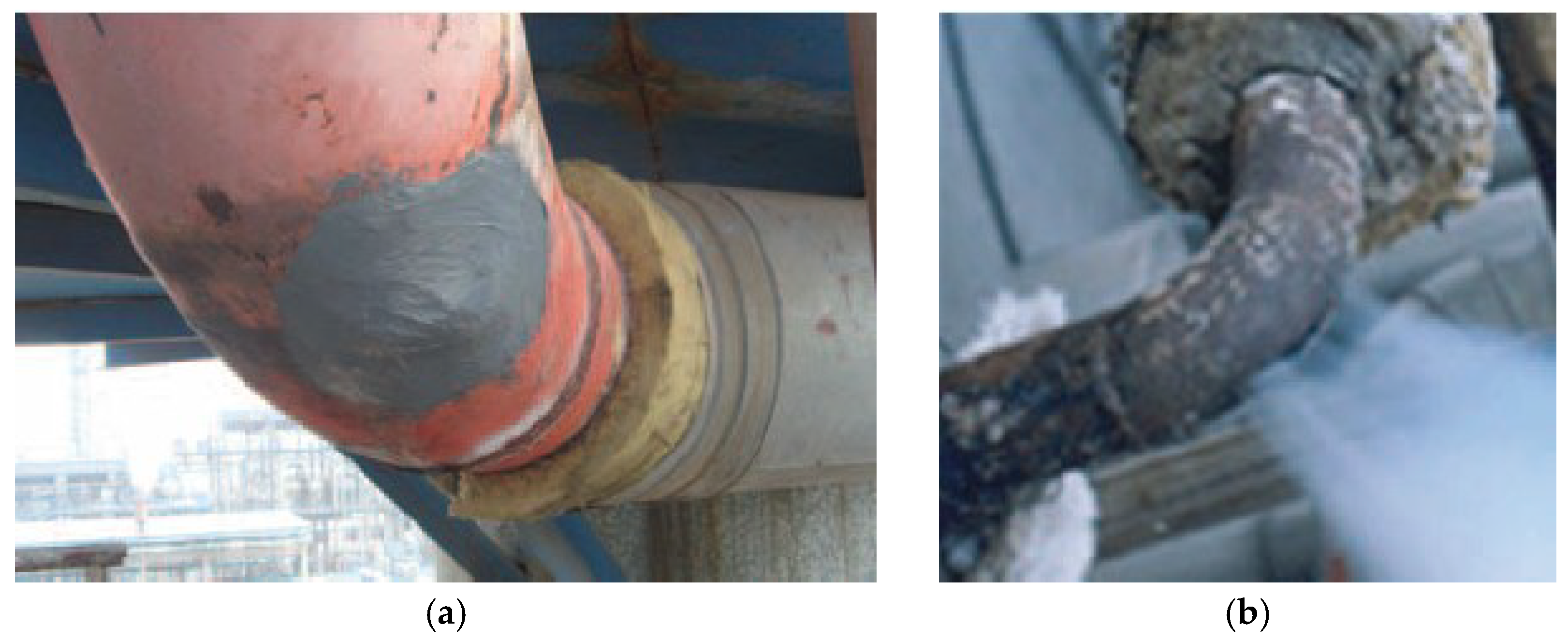With the deepening degree of erosion, the solid particles will eventually lead to pipeline leakage damage, influencing the environment and people’s life [3]. 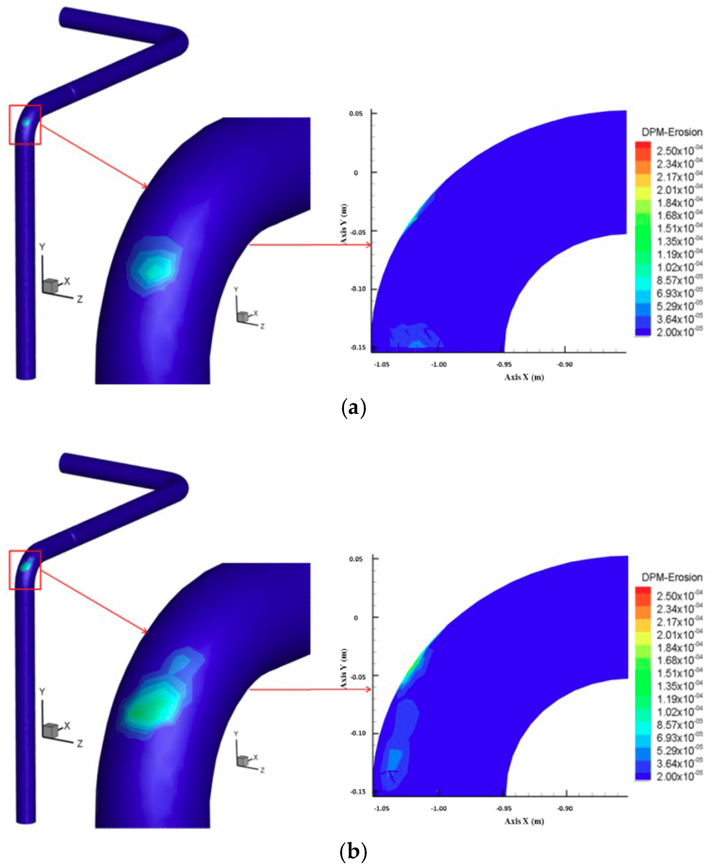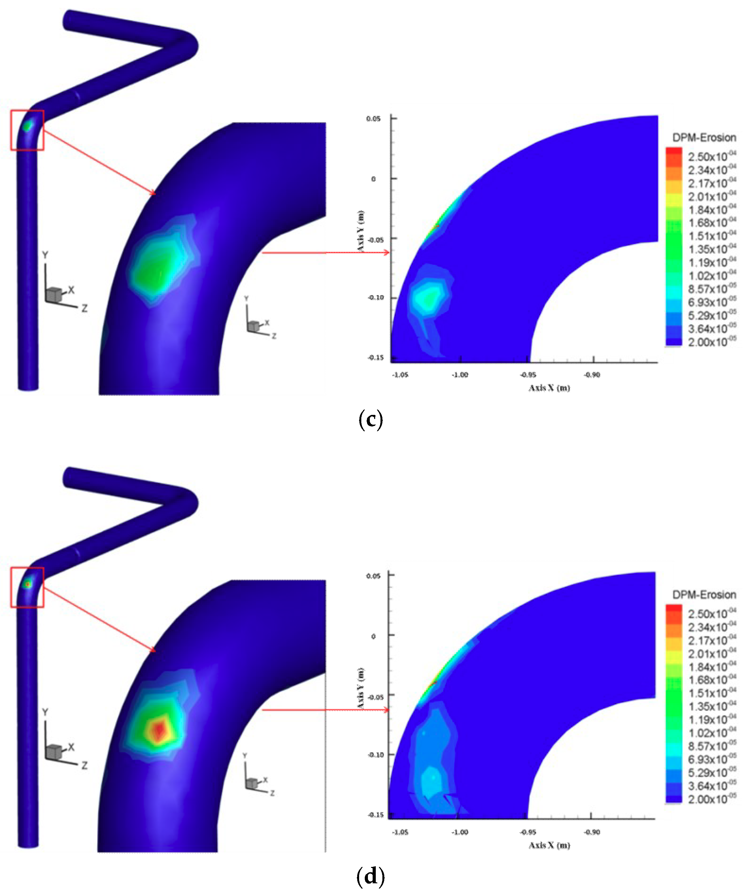Actual damaged pipelines are shown in Figure 1 [4]. Statistically, gas transmission stations in a given area, over six years, have undergone pipe perforations five times and serious pipe wall thinning three times. However, these pipe perforation events have not been identified in advance and serious pipe wall thinning events have been found occasionally in the process of station renovation. That is, on the one hand, pipe perforation and severe pipe wall thinning are of great safety concern for the gas transmission station operation; on the other hand, there have been no reliable methods to predict the degree of pipeline erosion.

According to the specific mechanism and experiment, experts and scholars at home and abroad in recent years have established different erosion theories and put forward different erosion rate predicting equations that consider various erosion parameters [3]. From the aspect of erosion theory, Bitter [5] proposed the theory of deformation wear from the viewpoint of energy balance, but this theory lacked the support of a physical model. Finnie [6] proposed a micro cutting theory that well explained the law of plastic material erosion under a low impact angle, but this theory was not suitable for brittle material erosion and plastic material erosion under high impact angle. Levy [7] proposed a theory of extrusion forging that only focused on high-impact-angle erosion. Tilly [8] studied the impact of plastic material erosion by particles and put forward a secondary erosion theory suited for brittle particles under high impact angle. From the aspect of erosion rate prediction, Oka et al. [9,10] put forward an E/CRC erosion wear experience relation equation that considers the target material hardness, particle diameter and particle properties. Lin [11] presented a relation function for erosion rate, particle size, flow and impact angle. API-14E [12] proposed an erosion velocity empirical formula that considered mixed fluid density, but the deviation of calculation results was bigger in the prediction of erosion speed under lower fluid mixing density. Desale et al. [13] put forward a relational expression for the erosion rate and particle size and pointed out that this expression was related to material properties, experimental conditions, particle velocity and particle size distribution. Ou et al. [14,15] studied the liquid phase distribution and the particle trajectory in gas-liquid-solid multiphase flow pipeline and then an erosion rate formula was put forward. Lian et al. [16] put forward a change curve for the erosion rate and angle of the bent sub after performing an erosion simulation for a sand piping bent sub. Gnanavelu et al. [17] obtained the schematic diagram of stainless steel wall erosion loss for different particle impact angles and the impact speeds by integrating experimental results and computational fluid dynamics simulation. Lester et al. [18] obtained a fitted formula for the thickness erosion loss including the particle impact velocity and angle through a matching experiment and computational fluid dynamics simulation data of liquid-solid two phase fluid on a cylinder sample. Feng et al. [19] applied a self-defining function to fix the initial erosion calculation model of computational fluid dynamics software (FLUENT) software, then studied the liquid-solid erosion rule in the sudden expansion and contraction pipe as well. Zhang et al. [20] predicted the wall erosion process and compared wall thickness erosion loss for bending tubes surface with different angles by simulating liquid-solid two-phase flow in bend tubes. Li et al. [21] found that the wall thickness erosion loss along with the increase of liquid phase velocity increased exponentially under the working condition of hydraulic fracturing in a restriction choke. Ran [22] proposed an erosion calculation model suitable for hydraulic jet fracturing conditions according to the rule of erosion damage and sand distribution in a dual-cluster hydraulic ejector.

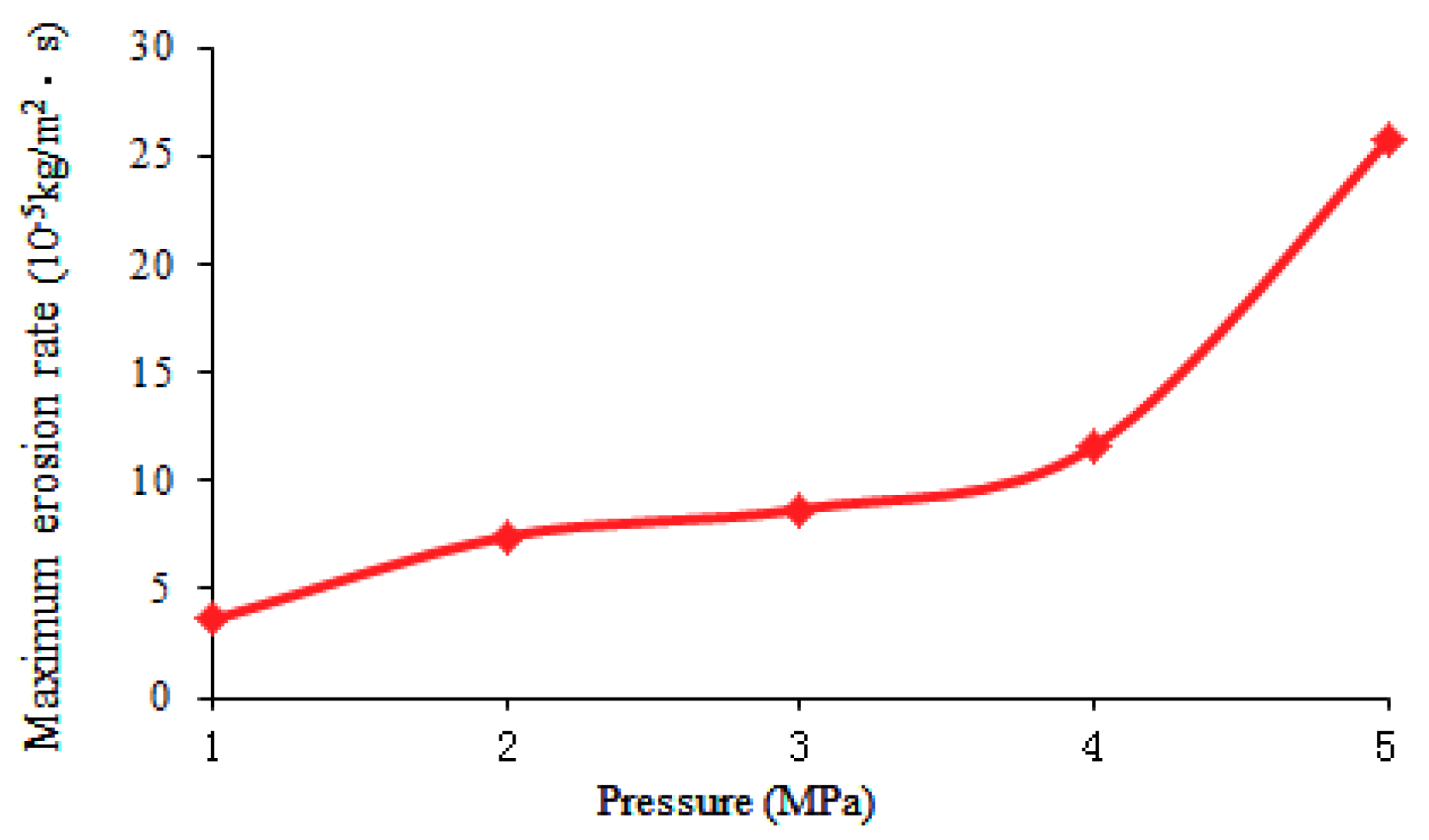
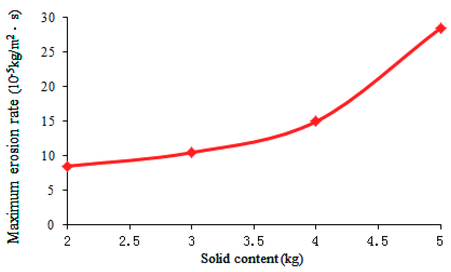
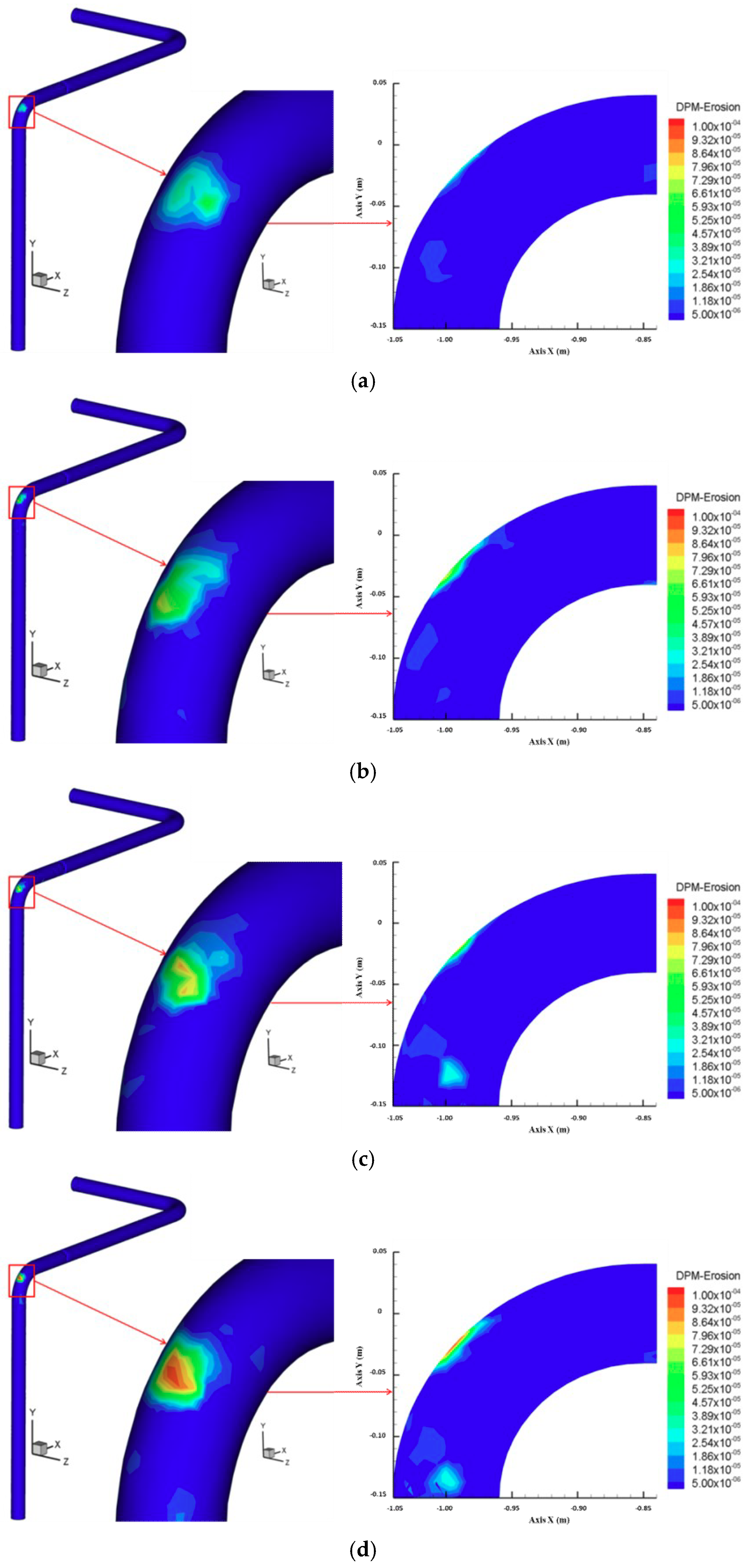
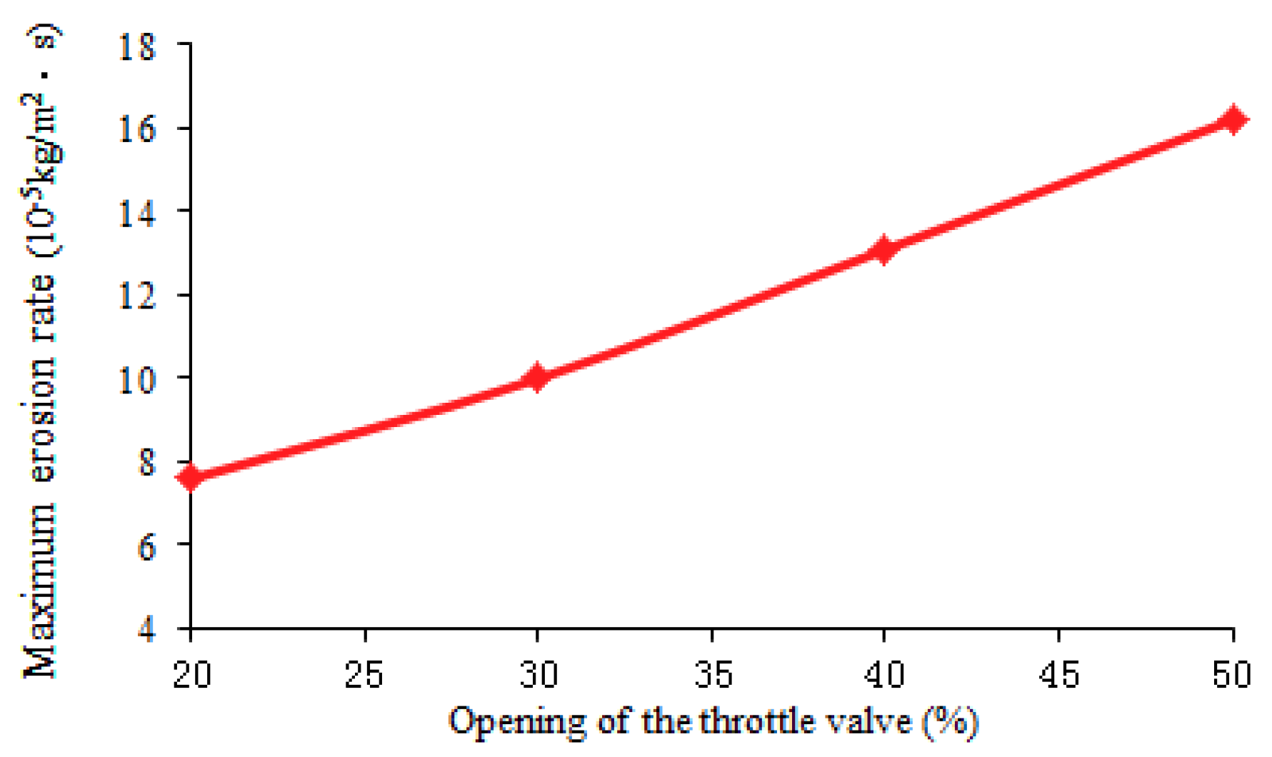
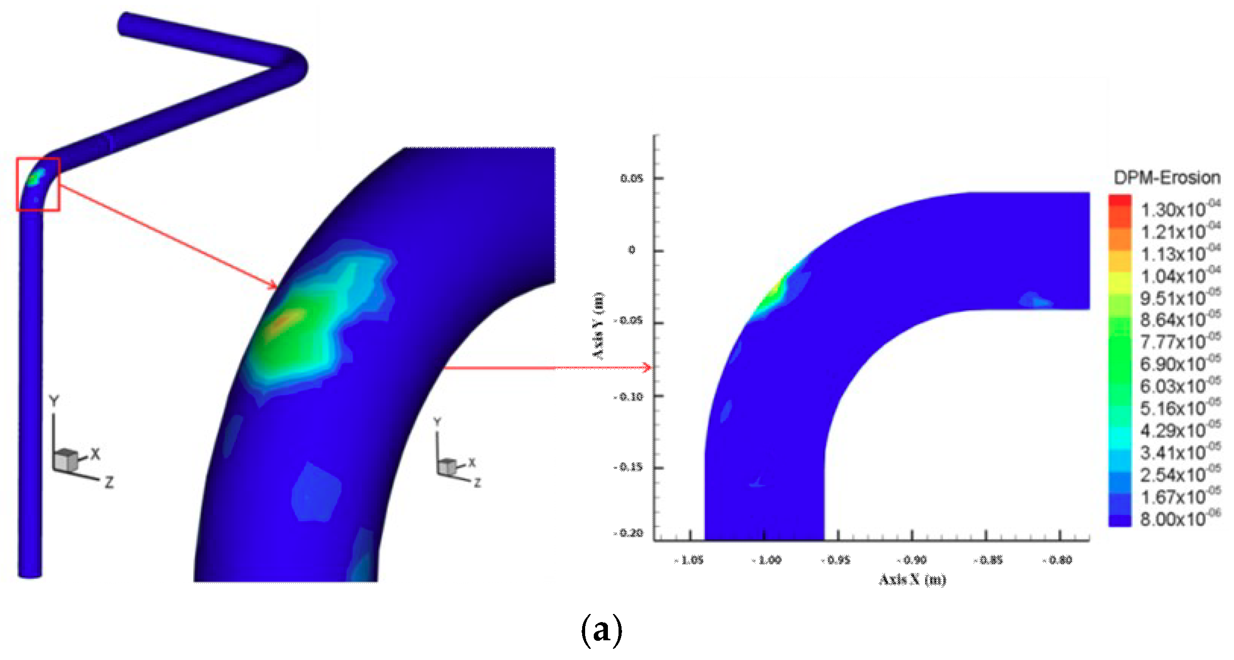
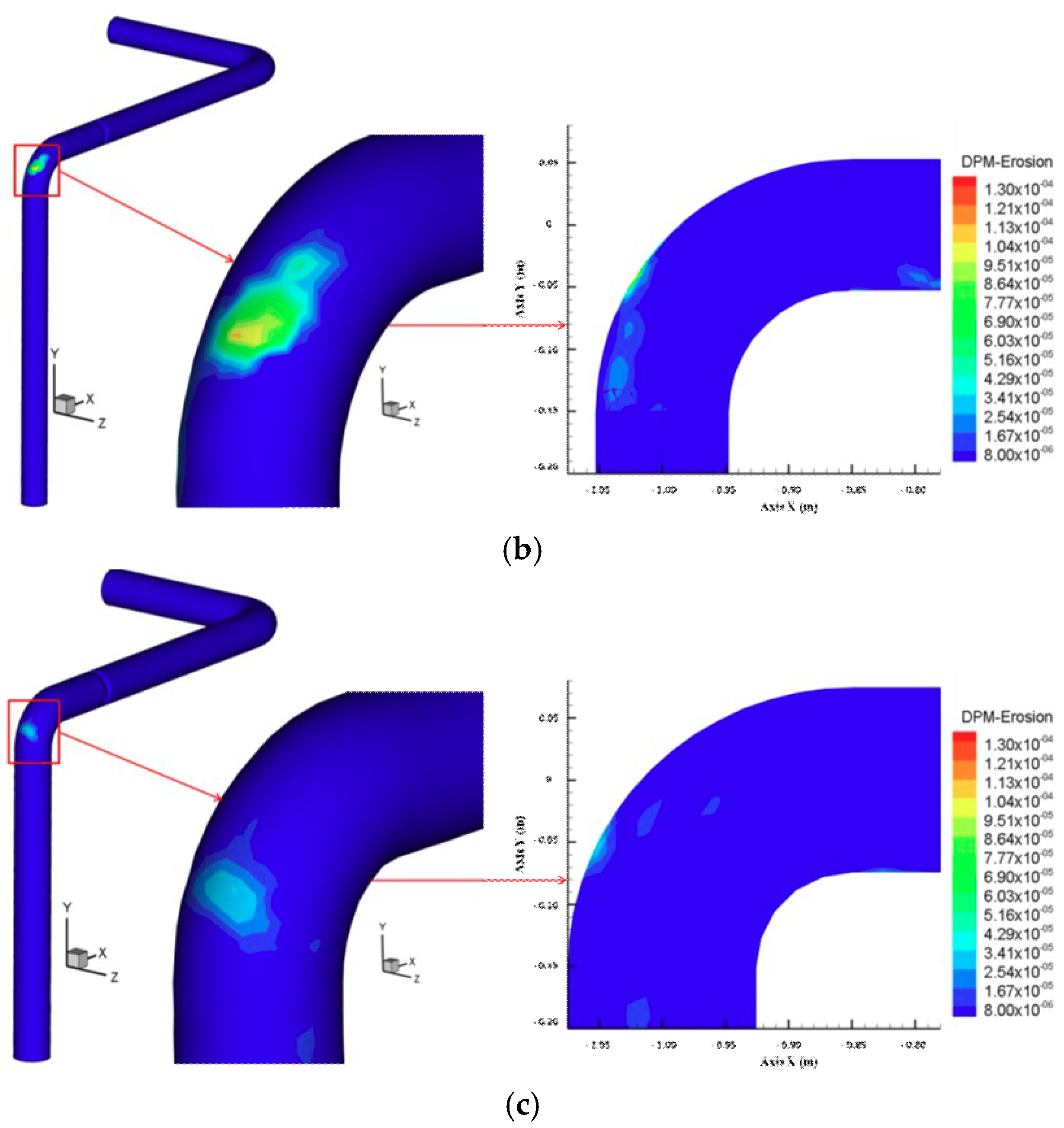
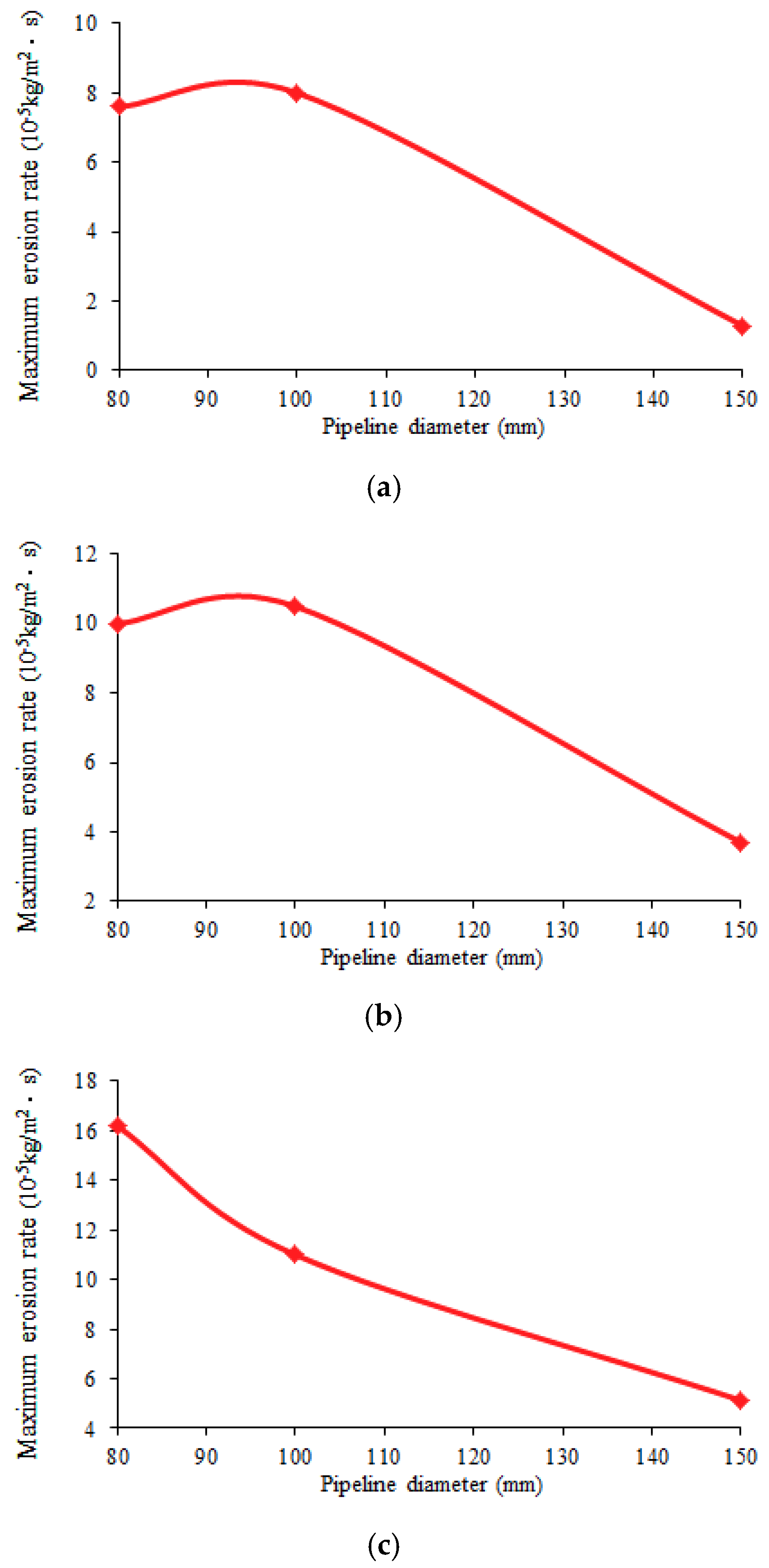
Although there are many studies on the liquid-solid two-phase flow erosion, nevertheless, research on Gas–Solid two-phase flow erosion is relatively lacking. In addition, because most research on Gas–Solid two-phase flow erosion is limited to the proposed parameter conditions, it is difficult to combine research results with actual working conditions. Therefore, a recognized and widely applicable prediction method for the production field to accurately forecast the erosion level of material is lacking. Consequently, according to the erosion characteristics of pipeline material, it is necessary to establish a maximum erosion rate prediction equation for the Gas–Solid two-phase flow pipe widely used for engineering application in gas transmission stations by simulating the environment closer to actual operation conditions.

2. Gas–Solid Two-Phase Pipeline Erosion Model

2.1. Erosion Physical Model

Gas–Solid two-phase flow pipeline in a gas transmission station is composed of pipe sections and valves. As shown in Figure 2, a double-valve structure and a right angle bend is designed for the Gas–Solid two-phase flow pipeline, namely, a brake valve and a throttle valve successively from the upstream to downstream, with a pipe bending angle of 90°.

2.2. Fluid Dynamics Theory

2.2.1. Gas Phase Equations

To simulate the erosion behavior under the action of gas–solid two-phase flow in a pipeline, the gas–solid two-phase flow pipe erosion model is established using the finite element method.

The gas phase as a continuous phase is solved by using the Navier–Stokes equation. The gas-phase control equations are as follows:

$$\frac{\partial {\rho }_{\mathrm{g}}}{\partial t}+\frac{\partial }{\partial x_i}\left({\rho }_{\mathrm{g}}{v}_i\right)=0$$

(1)

$$\frac{\partial }{\partial t}\left({\rho }_{\mathrm{g}}{v}_i\right)+\frac{\partial }{\partial x_j}\left({\rho }_{\mathrm{g}}{v}_i{v}_j\right)=-\frac{\partial p}{\partial x_i}+\frac{\partial {\tau }_{ij}}{\partial x_j}+{\rho }_{\mathrm{g}}{g}_i+F_i$$

(2)

where ρ_g is the density of the gas phase, t is time, p is the pressure, v_i is the instantaneous velocity vector, τ_ij is the stress tensor, ρ_gg_i is gravity for the direction i, and F_i is the additional source term of acting on continuous phase by particles.

The main form of fluid flow in the pipeline is turbulence. Momentum, energy, and concentration are mutually exchanged in the fluid medium by fluid fluctuations, especially in the area where the pipeline geometry varies and the fluid velocity is high.

Based on fluid dynamics, the Re-normalization group (RNG) k–ε turbulent flow model with a better simulation for separate and secondary flow turbulent flow is adopted. In addition, constants of this model are precisely deduced from RNG model so as to be fit to the study of Gas–Solid two phase flow pipeline erosion. The turbulence model is as follows [23]:

$$\{\begin{array}{c}\frac{\partial \left({\rho }_{\mathrm{g}}k\right)}{\partial t}+\frac{\partial \left({\rho }_{\mathrm{g}}k{v}_i\right)}{\partial x_i}=\frac{\partial }{\partial x_j}\left({\alpha }_k{\mu }_{\mathrm{eff}}\frac{\partial k}{\partial x_j}\right)+G_k+G_{\mathrm{b}}-{\rho }_{\mathrm{g}}\epsilon -Y_{\mathrm{M}}+S_k\\ \frac{\partial \left({\rho }_{\mathrm{g}}\epsilon \right)}{\partial t}+\frac{\partial \left({\rho }_{\mathrm{g}}\epsilon v_i\right)}{\partial x_i}=\frac{\partial }{\partial x_j}\left({\alpha }_{\mathsf{\epsilon }}{\mu }_{\mathrm{eff}}\frac{\partial \epsilon }{\partial x_j}\right)+C_{1\epsilon }\frac{\epsilon }{k}\left(G_k+C_{3\epsilon }{G}_{\mathrm{b}}\right)-C_{2\epsilon }{\rho }_{\mathrm{g}}\frac{{\epsilon }^2}{k}-R_{\epsilon }+S_{\epsilon }\end{array}$$

(3)

where k is the turbulent kinetic energy, ε is the turbulent dissipation rate, μ_eff is the effective viscosity, G_k is the turbulent kinetic energy produced by laminar flow velocity gradient, G_b is the turbulence kinetic energy produced by buoyancy, Y_M is the fluctuation contribution value produced by excessive diffusion in compressible turbulence, x_i and x_j are the space coordinate (i ≠ j), α_k and α_ε are the turbulent Prandtl number in the direction k and ε, S_k and S_ε are the correction term related to practical problems, and C_1ε, C_2ε and C_3ε are experience constants, R_ε is the function of ε.

2.2.2. Solid Phase Equations

Assuming that the solid phase is an irregular sphere and that particle collisions will not result in pipeline deformation, the solid phase is considered as a discrete phase. The equation of motion for solid particles is as follows [23]:

$$\frac{d{v}_{\mathrm{s}}}{dt}=\frac{18\mu }{{\rho }_{\mathrm{s}}{d}_{\mathrm{s}}^2}\frac{C_{\mathrm{D}}{\mathrm{Re}}_{\mathrm{s}}}{24}\left(v_{\mathrm{g}}-v_{\mathrm{s}}\right)+\frac{g_x\left({\rho }_{\mathrm{s}}-{\rho }_{\mathrm{g}}\right)}{{\rho }_{\mathrm{s}}}+F_x$$

(4)

where:

$${\mathrm{Re}}_{\mathrm{s}}=\frac{{\rho }_{\mathrm{g}}{d}_{\mathrm{s}}\left|v_{\mathrm{s}}-v_{\mathrm{g}}\right|}{\mu }$$

(5)

where v_g is the gas phase velocity, v_s is the particle velocity, ρ_s is the particle density, d_s is the particle diameter, Re_s is the relative Reynolds number, C_D is the drag coefficient, $g_x({\rho }_{\mathrm{s}}-{\rho }_{\mathrm{g}})/{\rho }_{\mathrm{s}}$ is the resultant force of unit particle quality by gravity and buoyancy, and F_x is the force of unit particle quality including an additional quality force, pressure gradient force, Basset force, and Saffinan lift etc. This last term can be ignored, as the density of solid particles is far greater than the gas density.

For irregular spherical particles, the drag coefficient C_D is calculated according to the following formula [23]:

$$C_{\mathrm{D}}=\frac{24}{{\mathrm{Re}}_{sph}}\left(1+b_1{\mathrm{Re}}_{sph}^{b_2}\right)+\frac{b_3{\mathrm{Re}}_{sph}}{b_4+{\mathrm{Re}}_{sph}}$$

(6)

where:

$$\{\begin{array}{l}{b}_1=\exp \left(2.3288-6.4581\varphi +2.4486{\varphi }^2\right)\\ b_2=0.0964+0.5565\varphi \\ b_3=\exp \left(4.905-13.8944\varphi +18.4222{\varphi }^2-10.2599{\varphi }^3\right)\\ b_4=\exp \left(1.4681+12.2584\varphi -20.7322{\varphi }^2+15.8855{\varphi }^3\right)\end{array}$$

(7)

$$\varphi =\frac{s}{S}$$

(8)

where s is the surface area of a sphere of the same volume as the particles, S is the actual surface area of particles, and Re_sph is the Reynolds number calculated by using the equivolume sphere diameter.

2.3. Finite Element Model

2.3.1. Finite Element Model and Grid Division

In the process of solid discharge in a gas transmission station, the emission rate is controlled by adjusting the opening of the throttle valve while the brake valve is fully open. In accordance with actual blowdown operation in a gas transmission station, multiple geometric models and finite element models, classified by the opening of the throttle valve and pipe size, are established. In the geometric model, there are two bent pipes with 90° angles marked A and B along the flow direction and five straight pipes marked L1–L5 whose pipe lengths are listed in

Table 1. Straight pipe length of a gas–solid two-phase pipeline.

L1 (cm)	L2 (cm)	L3 (cm)	L4 (cm)	L5 (cm)
80	40	80	40	140

. In this paper, we focus on three types of pipe size—DN80 (D88.9 × 4), DN100 (D114.3 × 4.5), and DN150 (D159 × 5) —and three forms of throttle valve openings: 20%, 30%, and 50%. (Note that, when the throttle valve is fully open, its circulation area accounts for 43% of the pipeline’s total circulation area. Given equal proportion flow coefficients, the circulation area of the throttle valve accounts 9%, 13%, and 22% of the pipeline’s total circulation area for throttle valve openings of 20%, 30%, and 50%, respectively). According to the test report of particle size in gas transmission station, the range of particle size is 0−60 μm and the average particle size is 20 μm. So, in our simulation, we set the particle size to 20 μm. The type of solid is FeS whose density is obtained from particle test report. The type of gas is set as methane whose density and viscosity are gotten from the quality inspection report of natural gas. In the finite element models, hexahedral mesh is adopted especially mesh encryption in pipe bend. Figure 3 shows the geometric model and the erosion model for gas–solid two-phase flow pipeline with a DN100 pipe and a throttle valve opening of 30%. The finite element models were proposed by using ANSYS FLUENT software (ANSYS, Inc., Canonsburg, PA, USA), as shown in Figure 3, the number of grid is 1,045,741, and the number of grid nodes is 1,010,288. In this model, the discrete phase model and the viscous model were used in one emission. In the discrete phase model, the drag law is choosing the nonspherical item, shape factor is set as 0.8, the physical model is choosing the erosion/accretion item. In the viscous model, the k–ε turbulent flow model is used and the near-wall treatment is set to standard wall functions.

2.3.2. Boundary Conditions

On the one hand, data from pressure gauges upstream of the equipment are the actual data that can be directly obtained in the field. Moreover, the end of the drainage pipe accesses the blowdown tank whose back pressure is atmospheric pressure. On the other hand, a solid emission force is coming from the real-time operation pressure of the equipment and the emission rate is controlled by adjusting the opening of the throttle valve while the brake valve is fully open. Therefore, for the Gas–Solid two-phase flow pipeline erosion simulation, the inlet boundary condition is a pressure condition and the outlet boundary condition is a free flow boundary.

2.3.3. Numerical Calculation

With the influence of gravity on the fluid flow taken into account, the RNG k–ε turbulence model is used to calculate the gas continuous phase and the DPM (Discrete Phase Model) is applied to solve for the solid discrete phase. In this paper, the Eulerian–Lagrangian method is used. Thus, the gas continuous phase flow field is obtained by solving the gas phase control equations in an Eulerian coordinate system and the solid discrete phase trajectory is obtained by using a random trajectory model in the Lagrangian coordinate system. The two-way coupling calculations of mass, momentum, and energy exchange between the continuous phase and the discrete phase are realized by alternately solving control equations for the gas phase and the motion equation for the solid phase [23].

(1) Quality exchange

The quality exchange quantity from the discrete phase to the continuous phase is equal to the variable quantity of particle quality, when particles pass through a control volume:

$$M=\frac{\Delta m_s}{m_{s,0}}{\dot{m}}_{s,0}$$

(9)

where m_s,0 is the initial quality of particles and ${\dot{m}}_{s,0}$ is the initial mass flow rate of particles.

(2) Momentum exchange

Within a time step ∆t, the momentum exchange quantity between the discrete phase and the continuous phase is equal to the variable quantity of particle momentum in a control volume:

$$F={\displaystyle \sum \left[\frac{18\mu }{{\rho }_s{d}_s^2}\frac{C_D{\mathrm{Re}}_s}{24}\left(v_s-v_g\right)+f_x\right]}{\dot{m}}_s\Delta t$$

(10)

where f_x is other forces and ${\dot{m}}_s$ is the particle mass flow rate.

The coupling between velocity field and pressure field is solved by using SIMPLE algorithm. The pressure correction equation derived by the continuity equation is as follows [24]:

$$a_{i,j}{P}_{i,j}^{\text{'}}=a_{i+1,j}{P}_{i+1,j}^{\text{'}}+a_{i-1,j}{P}_{i-1,j}^{\text{'}}+a_{i,j+1}{P}_{i,j+1}^{\text{'}}+a_{i,j-1}{P}_{i,j-1}^{\text{'}}+b_{i,j}^{\text{'}}$$

(11)

where:

$$\{\begin{array}{l}{a}_{i+1,j}={\left(\rho dA\right)}_{i+1,j}\\ a_{i-1,j}={\left(\rho dA\right)}_{i-1,j}\\ a_{i,j+1}={\left(\rho dA\right)}_{i,j+1}\\ a_{i,j-1}={\left(\rho dA\right)}_{i,j-1}\\ a_{i,j}=a_{i+1,j}+a_{i-1,j}+a_{i,j+1}+a_{i,j-1}\\ b_{i,j}^{\text{'}}={\left(\rho v^{*}A\right)}_{i,j}-{\left(\rho v^{*}A\right)}_{i+1,j}+{\left(\rho v^{*}A\right)}_{i,j+1}-{\left(\rho v^{*}A\right)}_{i,j-1}\end{array}$$

(12)

where P′ is the pressure correction value, v* is the initial velocity distribution, and b′_i,j is the unbalanced flow rate caused by the correction of the velocity field. In this paper, the convergence condition for the iterative calculation is b′_i,j tending to zero.

2.4. Erosion Rate Calculation Method

In practical production, the pipe wall annual thinning thickness is used to characterize the erosion degree induced by gas–solid two-phase flow pipeline. Therefore, the conversion formula for the simulation data is as follows:

$$Y=\frac{60,000nxt}{\rho }$$

(15)

where Y is the annual erosion rate, n is the equipment blowdown frequency in a year, x is the pipe erosion rate in one emission by simulation, t is the equipment blowdown period, and ρ is the density of pipe steel.

Regarding the equipment blowdown frequency and period, there is an example to demonstrate how to determine. In general, there are at least three separators in a gas transmission station, only two separators are operating at any time, and the other one is spare separator. For two operating separators, the blowdown frequency is one time per week, and the blowdown period is approximately 6 min for every time. Meanwhile, the spare separator is usually alternated quarterly. In three years, each separator experiences approximately 96 times blowdown operating. In other words, the average blowdown frequency is approximately 32 times per year. Thus, the blowdown frequency should be 32 times/year, and the equipment blowdown period should be 6 min.

2.5. Analysis of Grid Independence

Taking DN100 two-phase flow pipeline as an example, in order to verify the accuracy of numerical calculations and the increase of grid number will not have a significant impact on the simulation results, seven different numbers of grids have been created in the finite element models. Then, the model with different number of grids is simulated under the same boundary condition of 3.0 MPa, 3.0 kg of solid content and 30% of the throttle valve opening, and the maximum erosion rate is taken as the comparison object. The maximum erosion rate with different numbers of grids is shown in Figure 4. The result shows that the maximum erosion rate gradually increases with the grid number increasing, and when the grid number reaches 1,045,741, the maximum erosion rate has no obvious change. Therefore, it is considered that the requirement of mesh independence is achieved when the grid number of the erosion model is about 1,045,741.

2.6. Model Validation

In order to validate the numerical simulation results, we compared the calculating results to the actual working condition. In order to obtain the erosion data of the pipeline in gas transmission station, the MMX-6 Type Ultrasonic Thickness Gauge (Dakota Co., Eagan, MA, USA) was used to monitor the wall thickness of the pipeline in gas transmission station K (denote as Field K) that located in Sichuan area. There are three separators in this gas transmission station, each separator connects with the gas pipeline. For each bend pipeline, the position distribution of detection points is shown in Figure 5, 13 loops were tested for key points (welding line, bend pipe, throttle valve), and each loop sets 8 detection points. Due to the manufacturing process, the wall thickness of the intrados of bend pipe is usually greater than that of the outer, thus, the detection points 4–6 did not measured. The original testing data are given in Appendix A (see

Table A1. Testing results for Field K.

No.	Wall Thickness (mm)
	1	2	3	4	5	6	7	8
F-1	4.584	4.675	4.820	/	/	/	4.823	4.678
F-2	4.623	4.676	4.817	/	/	/	4.818	4.673
F-3	4.619	4.677	4.816	/	/	/	4.814	4.675

).

But the original wall thickness of the bend pipe was not measured and recorded, thus, the testing results of the wall thickness need to be processed to determine the thickness reduction of the bend pipe. In order to ensure the consistency of wall thickness data, the data processing method for testing results is given as follows: (1) Calculate the average wall thickness from detection points 2, 3, 7, 8 of each loop to obtain the initial wall thickness, due to these points are seldom subjected to the erosion of gas–solid two-phase flow; (2) Calculate the minimum wall thickness from detection points 1–8 of each loop to obtain the remaining wall thickness after the erosion of gas–solid two-phase flow; (3) Calculate the maximum reduction of wall thickness for each loop; (4) Calculate the maximum erosion rate, it is the ratio of the maximum decrement to the operating years. According to the testing results, we found that the most serious erosion area occurred at the outer cambered surface of bend after throttle valve. Thus, we just utilized the testing results of loop 10^th as the field testing results, by taking the gas–solid two-phase flow pipeline in gas transmission station equipment as the research object, the calculation results simulated for actual working condition and the actual wall thickness test data are compared, and the results are listed in

Table 2. Calculation results and test data comparison.

No.	Max. Erosion Rate (mm/year)		Error (%)	Remarks
	Test Data	Calculation Results
F-1	0.1650	0.1541	6.61	In the initial operation stage, openings of 20%, pressure of 3.77 MPa, solid content of 2.63 kg, blowdown period of 8min, blowdown operation of 48 times, the most serious erosion area occurred at the outer cambered surface of bend after throttle valve
F-2	0.1230	0.1346	−9.43	In the middle operation stage, openings of 30%, pressure of 3.75 MPa, solid content of 2.2 kg, blowdown period of 6.5 min, blowdown operation of 32 times, the most serious erosion area occurred at the outer cambered surface of bend after throttle valve
F-3	0.1265	0.1401	−10.75	In the middle operation stage, openings of 50%, pressure of 3.74 MPa, solid content of 2.0 kg, blowdown period of 5.7 min, blowdown operation of 32 times, the most serious erosion area occurred at the outer cambered surface of bend after throttle valve

, where F-1, F-2 and F-3 represent the connected bend pipeline for three separators. In addition, the maximum erosion rate also should be converted to the unit of mm/year by using Equation (15). It can be seen from Table 2 that (1) the absolute percentage error of the maximum erosion rate between the model calculation results and the field test datum is ≤10.75%; (2) the most serious erosion area determined by the erosion model is located in the outer cambered surface of the bend after the throttle valve, which is the same as what is found in the test results. That is, the gas–solid two-phase flow pipeline erosion behaviors can be accurately simulated by the established erosion model so as to provide a theoretical basis for pipeline maintenance in a gas transmission station.

3. Simulation Results and Discussions

The erosion characteristics of gas–solid two-phase flow pipeline have been simulated with different pressures, solid contents, throttle valve openings, and pipe diameters. The laws for the most serious erosion area and the maximum erosion rate as a function of pressure, solid content, throttle opening and pipe diameter are then analyzed.

3.1. Influence of Pressure

For a certain solid content, opening of the throttle valve, and pipe diameter, the laws of the most serious erosion area and maximum erosion rate varying with pressure are the same. Under the condition of 3.0 kg of solid content, 30% of the throttle valve opening, and DN100 as an example, the most serious erosion area and maximum erosion rate with pressure varying from 1.0 to 5.0 MPa are shown in Figure 6 and Figure 7.

As shown in Figure 6 and Figure 7, it can be seen that: (1) the maximum erosion rate increases with pressure rising. The influence of pressure on erosion rate is mainly manifested on the gas velocity. When the gas flow rate increases with pressure rising, the gas velocity increases. On the one hand, it makes the solid carrying capacity of gas enhance so as to increase the particle kinetic energy which leads to the contact pressure bigger on the pipe wall. On the other hand, it makes particles collide with the pipe wall more frequently. So under the effect of two factors together, the maximum erosion rate increases with pressure rising. (2) The most serious erosion area is located in the outer cambered surface of the bend after the throttle valve and it never changes with regardless of the pressure. This is because solid particles are carried by gas, their space distribution depends largely on the internal flow field characteristics of the gas. Regardless of the pressure changes, the solid particles always follow the gas flow in the straight pipe and barely collide with the pipe wall. But near the 90° bent pipe, because the flow line rapidly turns, speed concentration and strong turbulence arise, it leads to particles directly collide with the pipeline wall. Thus, serious erosion occurs in the outer cambered surface of the bend. Moreover, due to the decompression effect of the throttle valve, the pressure after the throttle valve rapidly reduces which lead to the gas velocity increases sharply so as to make the erosion rate of the bend pipe after throttle valve is greater than the one before throttle valve. In other words, the maximum erosion is mainly induced by the combined action of bend pipe and throttle valve.

3.2. Influence of Solid Content

For a certain pressure, opening of the throttle valve, and pipe diameter, the laws of the most serious erosion area and maximum erosion rate varying with solid content are the same.

Under the condition of 3.5 MPa, 30% of the throttle valve opening, and DN100 as an example, the most serious erosion area and maximum erosion rate with the solid content varying from 2.0 to 5.0 kg are shown in Figure 8 and Figure 9. As shown in Figure 8 and Figure 9, it can be seen that (1) the maximum erosion rate increases with increasing solid content. This is because when the solid content increases, the solid concentration in Gas–Solid two-phase flow increases, which makes the frequency of particles colliding with the pipe wall increase, and the impact action on the pipe wall also enhance. That is, the maximum erosion rate increases with solid content increasing. (2) The most serious erosion area is located in the outer cambered surface of the bend after the throttle valve and it never changes regardless of the solid content. This is because solid particles are carried by gas, their space distribution depends largely on the internal flow field characteristics of the gas. Regardless of the solid content changes, the solid particles always follow the gas flow in the straight pipe and barely collide with the pipe wall, and the maximum erosion is always occurred at the outer cambered surface of bend after the throttle valve due to the combined action of bend pipe and throttle valve.

3.3. Influence of the Throttle Valve Opening

For a certain pressure, solid content, and pipe diameter, the laws of the most serious erosion area and maximum erosion rate varying with the opening of the throttle valve are the same. Under the condition of 3.5 MPa, 3.0 kg of solid content, and DN80 as an example, the most serious erosion area and maximum erosion rate with the opening of the throttle valve varying from 20% to 50% are shown in Figure 10 and Figure 11.

It can be seen from the Figure 10 and Figure 11 that: (1) the maximum erosion rate increases with the opening of the throttle valve increasing. The Gas–Solid two-phase flow rate is changeless under the precondition of certain pressure and solid content. With increasing of the opening of the throttle valve, the choking effect of the valve throttle is reduced. On the one hand, the gas velocity increases and the solid carrying capacity of gas enhance, due to the increase in two-phase flow rate after the throttle valve. Then, the increase of particle kinetic energy leads to the contact pressure bigger on the pipe wall. On the other hand, the pressure drop gradient after the throttle valve increases, which makes the gas velocity gradient increase. The increase of the gas velocity gradient also causes fluid turbulence intensity enhances, and then leads to the increase in the frequency of particles colliding with the pipe wall. So under the effect of two factors together, the maximum erosion rate increases with the opening of the throttle valve increasing. (2) The most serious erosion area is located in the outer cambered surface of the bend after the throttle valve and it never changes regardless of the throttle valve opening. This is because solid particles are carried by gas, their space distribution depends largely on the internal flow field characteristics of the gas. Regardless of the throttle valve opening changes, the solid particles always follow the gas flow in the straight pipe and barely collide with the pipe wall, and the maximum erosion is always occurred at the outer cambered surface of bend after the throttle valve due to the combined action of bend pipe and throttle valve.

3.4. Influence of Pipe Diameter

The erosion rate of gas–solid two-phase flow pipeline is affected by fluid velocity and particulate dissemination. But influenced by the throttle valve opening, the two factors which plays the leading role is different with different pipe diameters. Therefore, under the condition of 3.5 MPa, 3.0 kg of solid content, and the throttle valve opening from 20% to 50% as an example, the most serious erosion area and maximum erosion rate with pipe diameter varying from DN80 to DN150 are shown in Figure 12, Figure 13, Figure 14 and Figure 15.

Under the precondition of certain pressure and solid content, as the pipe diameter increases, the increase in the two-phase flow rate leads to increased fluid velocity; however, the dispersity of particulates impacting the pipe wall is enhanced. Consequently, the laws for the maximum erosion rate as a function of pipe diameter are different under different throttle valve openings. It can be seen from Figure 12, Figure 13, Figure 14 and Figure 15 that (1) the maximum erosion rate increases at first and then decreases with pipe diameter increasing for throttle valve openings of 20% and 30%, and it decreases with pipe diameter increasing for a throttle valve opening of 50%. This is because, for throttle valve openings of 20% and 30%, the increase in gas velocity plays a dominant role when the pipe diameter increases from DN80 to DN100. The increasing of gas velocity makes the solid carrying capacity of gas enhance so as to increase the particle kinetic energy which leads to the contact pressure bigger on the pipe wall. However, the particle dispersion plays a leading role when the pipe diameter increases from DN100 to DN150. The increasing of particle dispersion leads the colliding effect of particles on the wall becomes dispersed. In other word, the maximum erosion rate decreases. In addition, for a throttle valve opening of 50%, the particle dispersion always plays a leading role with the increase of pipe diameter from DN80 to DN150. Therefore, it leads the colliding effect of particles on the wall become dispersed which is characterized by the increase of pipe diameter, the maximum erosion rate decreases. (2) The most serious erosion area is located in the outer cambered surface of the bend after the throttle valve and it never changes regardless of the pipe diameter. This is because solid particles are carried by gas, their space distribution depends largely on the internal flow field characteristics of the gas. Regardless of the pipe diameter changes, the solid particles always follow the gas flow in the straight pipe and barely collide with the pipe wall, and the maximum erosion is always occurred at the outer cambered surface of bend after the throttle valve due to the combined action of bend pipe and throttle valve.

4. Prediction of Maximum Erosion Rate

4.1. Prediction Equation for the Maximum Erosion Rate

Combined with the erosion calculation results for gas–solid two-phase flow pipeline under actual working conditions, the maximum erosion rate prediction equation is put forward on the basis of pressure, solid content, opening. This prediction equation focus on the influence of the maximum erosion rate affected by process parameters which are controllable on site, so the particle effect on erosion rate does not consider specially, the equation is given as follows:

$$z=C^{2.6}{P}^{0.6}$$

(13)

$$x=\frac{0.94M}{3}\left(a{z}^3+b{z}^2+cz+d\right)$$

(14)

$$Y=\frac{60,000nxt}{\rho }$$

(15)

where C is the opening of the throttle valve, P is the pressure, z is the middle calculation coefficient, M is the solid content, and a, b, c and d are coefficients related to the pipe diameter for gas–solid two-phase flow pipeline, the values of which are listed in

Table 3. Coefficient values.

Pipe Diameter	a	b	c	d
DN80	0.0127	−0.0087	0.0019	9 × 10−6
DN100	0.0159	−0.0101	0.0018	3 × 10−5
DN150	0.002	−0.0015	0.0004	1 × 10−6

.

4.2. Verification of the Maximum Erosion Rate Prediction Equation

To verify the accuracy of the maximum erosion rate prediction equation for gas–solid two-phase flow in the pipeline of the gas transmission station, we still utilized the same method that presented in Section 2.6. The MMX-6 Type Ultrasonic Thickness Gauge (Dakota Co., USA) was used to monitor the wall thickness of the pipeline for gas transmission station A–J (denote as Field A–J) that located in Chongqing and Sichuan area. For each bend pipeline in different stations, the position distribution of detection points is still shown in Figure 5, 13 loops were tested for key points (welding line, bend pipe, throttle valve), and each loop sets 8 detection points. Due to the most serious erosion area always occurred at the outer cambered surface of bend after throttle valve, we just utilized the testing results of loop 10th as the field testing results. Because of the manufacturing process, the wall thickness of the intrados of bend pipe is usually different with the outer surface of bend pipe, thus, the detection points 4–6 did not measure. The original testing data for Fields A-F in Chongqing area are given in Appendix B (see

Table A2. Testing results for Fields A–F in Chongqing area.

No.	Wall Thickness (mm)
	1	2	3	4	5	6	7	8
A	4.14	4.66	4.81	/	/	/	4.84	4.67
B	4.98	5.84	6.05	/	/	/	6.1	5.86
C	5.92	6.3	6.42	/	/	/	6.46	6.36
D	4.49	4.65	4.85	/	/	/	4.86	4.62
E	5.68	5.88	6.11	/	/	/	6.16	5.94
F	6.06	6.16	6.33	/	/	/	6.30	6.17

), and the original testing data for Fields G-J in Sichuan area are given in Appendix B (see

Table A3. Testing results for Fields G–J in Sichuan area.

No.	Wall Thickness (mm)
	1	2	3	4	5	6	7	8
G	4.08	4.68	4.80	/	/	/	4.81	4.66
H	5.58	5.86	6.07	/	/	/	6.14	5.87
I	5.90	6.31	6.41	/	/	/	6.45	6.37
J	4.44	4.67	4.83	/	/	/	4.85	4.65

). The data processing method for testing results: (1) Calculate the average wall thickness from detection points 2, 3, 7, 8 to obtain the initial wall thickness, due to these points are seldom subjected to the erosion of gas–solid two-phase flow; (2) Calculate the minimum wall thickness from detection points 1–8 to obtain the remaining wall thickness after the erosion of gas–solid two-phase flow; (3) Calculate the maximum reduction of wall thickness. The calculation results simulated for actual working condition and the actual wall thickness test data are compared, and the results are listed in

Table 4. Verification results of the maximum erosion rate with field test data in Chongqing area.

Field	Test Results (mm)	Calculation Results (mm)	Error (%)	Remarks
A	0.61	0.59	−3.28	operation for 8 years, solid content of 3 kg, particle size of 20 μm, openings of 20%, DN80, pressure of 2.5 MPa
B	0.98	1.00	2.04	operation for 7 years, solid content of 4 kg, particle size of 20 μm, openings of 20%, DN100, pressure of 3.5 MPa
C	0.47	0.43	−8.51	operation for 14 years, solid content of 2.5 kg, particle size of 20 μm, openings of 30%, DN150, pressure of 3.5 MPa
D	0.26	0.27	3.85	operation for 5 years, solid content of 1 kg, particle size of 20 μm, openings of 35%, DN80, pressure of 1.6 MPa
E	0.34	0.36	5.88	operation for 11 years, solid content of 1 kg, particle size of 20 μm, openings of 20%, DN100, pressure of 2.5 MPa
F	0.18	0.20	11.11	operation for 10 years, solid content of 4.7 kg, particle size of 20 μm, openings of 20%, DN150, pressure of 2 MPa

and

Table 5. Verification results of the maximum erosion rate with field test data in Sichuan area.

Field	Test Results (mm)	Calculation Results (mm)	Error (%)	Remarks
G	0.66	0.64	−3.03	operation for 8 years, solid content of 3 kg, particle size of 20 μm, openings of 20%, DN80, pressure of 3 MPa
H	0.41	0.43	4.88	operation for 3 years, solid content of 4 kg, particle size of 20 μm, openings of 20%, DN100, pressure of 3.5 MPa
I	0.48	0.53	10.42	operation for 13 years, solid content of 3.5 kg, particle size of 20 μm, openings of 30%, DN150, pressure of 3 MPa
J	0.31	0.33	6.45	operation for 6 years, solid content of 1 kg, particle size of 20 μm, openings of 40%, DN80, pressure of 1 MPa

. As given in Table 4 and Table 5, the biggest absolute percentage error in the maximum erosion rate between the prediction equation calculation results and the field test datum only 11.11%.

5. Conclusions

(1)

The gas–solid two-phase flow pipe erosion finite element model established in this paper was validated combining with field test data. Verification results show that the absolute percentage error in the maximum erosion rate between the model results and the test datum is ≤10.75%.

(2)

When the solid emission force is coming from the real-time operational pressure of the equipment and the emission rate is controlled by adjusting the opening of the throttle valve while the brake valve is fully open, the outer cambered surface of the bend after the throttle valve is the most serious erosion area for gas–solid two-phase flow pipeline in a gas transmission station.

(3)

When the solid emission force is coming from the real-time operational pressure of the equipment and the emission rate is controlled by adjusting the opening of the throttle valve while the brake valve is fully open, the maximum erosion rate increases with increasing pressure, solid content, and opening of the throttle valve, but, along with the change in the pipe diameter, the maximum erosion rate increases at first and then decreases with increasing pipe diameter for throttle valve openings of 20% and 30%, and it decreases with increasing pipe diameter for a throttle valve opening of 50%.

(4)

The maximum erosion rate prediction equation, a function of four parameters (pressure, solid content, opening of the throttle valve, and pipe diameter), yields an absolute percentage error with the field test datum of ≤11.11%. The equation can be effectively used to improve the accuracy of predicting the gas–solid two-phase flow pipeline erosion rate in a gas transmission station.

References

1. Ying, H. The solution of oil and gas two phase flow pipeline internal corrosion rate prediction model. J. Oil Gas Technol. 2009, 31, 364–366. [Google Scholar]
2. Li, L.; Ji, Z.; Xu, Q.; Xiong, Z.; Li, F.; Kan, G. A novel on-line detector for solid particles in natural gas pipelines under high pressure: A case study. Nat. Gas Ind. 2012, 32, 81–84. [Google Scholar]
3. Achebo, J.I. Pipeline using the drift flux models based on eulerian continuum equations. In Proceedings of the World Congress on Engineering, London, UK, 1–3 July 2009; Int Assoc Engineers-iaeng, UNIT1, 1-F, 37-39 Hung to Road: Kwun Tong, Hong Kong, China, 2009. [Google Scholar]
4. Zhu, H.; Zhao, H.; Pan, Q.; Li, X. Coupling analysis of fluid-structure interaction and flow erosion of Gas–Solid flow in elbow pipe. Adv. Mech. Eng. 2014, 2014, 1–10. [Google Scholar] [CrossRef]
5. Bitter, J.G.A. A study of erosion phenomena. Wear 1963, 6, 5–21. [Google Scholar] [CrossRef]
6. Finnie, I. On the velocity dependence of the erosion of ductile metals by solid particles at low angles of incidence. Wear 1978, 48, 181–190. [Google Scholar] [CrossRef]
7. Levy, A. Solid Particle Erosion and Erosion-Corrosion of Materials; ASM International: Material Park, OH, USA, 1995. [Google Scholar]
8. Tilly, G.P. A two stage mechanism of ductile erosion. Wear 1973, 23, 87–96. [Google Scholar] [CrossRef]
9. Oka, Y.; Okamura, K.; Yoshida, T. Practical estimation of erosion damage caused by solid particle impact: Part 1: Effects of impact parameters on a predictive equation. Wear 2005, 259, 95–101. [Google Scholar] [CrossRef]
10. Oka, Y.; Yoshida, T. Practical estimation of erosion damage caused by solid particle impact: Part 2: Mechanical properties of materials directly associated with erosion damage. Wear 2005, 259, 102–109. [Google Scholar] [CrossRef]
11. Nan, L. Research of Effect of Particle Properties and Flow Field on Erosion in Gas Pipelines. Ph.D. Thesis, Beijing Jiaotong University, Beijing, China, 2017. [Google Scholar]
12. API Recommended Practice 14E. Recommended Practice for Design and Installation of Offshore Production Platform Piping Systems; American Petroleum Institute: Washington, DC, USA, 2007. [Google Scholar]
13. Desale, G.R.; Gandhi, B.K.; Jain, S.C. Particle size effects on the slurry erosion of aluminum alloy (AA 6063). Wear 2009, 266, 1066–1071. [Google Scholar] [CrossRef]
14. Ou, G.; Xu, G.; Zhu, Z.; Yang, J.; Wang, Y. Fluid-structure interaction mechanism and numerical simulation of elbow erosion failure. J. Mech. Eng. 2009, 45, 119–124. [Google Scholar] [CrossRef]
15. Ou, G.; Qiu, J.; Zhu, Z.; Wang, Y.; Xu, G. Fluid-structure interactional numerical simulation of erosion-corrosion failure of reducer in multiphase flow. Chin. J. Theor. Appl. Mech. 2010, 42, 197–204. [Google Scholar]
16. Lian, Z.; Chen, X.; Lin, T.; Ming, X.; Zheng, J. Study on erosion mechanism of bending joint in blooey line. J. Southwest Pet. Univ. (Sci. Technol. Ed.) 2014, 36, 150–156. [Google Scholar]
17. Gnanavelu, A.; Kapur, N.; Neville, A.; Flores, J.F. An integrated methodology for predicting material wear rates due to erosion. Wear 2009, 267, 1935–1944. [Google Scholar] [CrossRef]
18. Lester, D.R.; Graham, L.A.; Wu, J. High precision suspension erosion modeling. Wear 2010, 269, 449–457. [Google Scholar] [CrossRef]
19. Feng, L.; Wang, J.; Mao, Y.; Zhang, G.; Wang, J. Numerical simulation of liquid-solid erosion in sudden expansion and contraction tube. Acta Petrolei Sinica (Pet. Process. Sect.) 2014, 30, 1080–1085. [Google Scholar]
20. Zhang, S.; Cao, H.; Liu, Y.; Gao, C. Numerical simulation of liquid-solid two-phase flow and erosion-collision in a syphon. J. Hebei Univ. Technol. 2008, 37, 48–54. [Google Scholar]
21. Li, G.; Wang, Y.; Sun, H.; Kang, L.; Wang, Y.; He, R. Numerical simulation on solid particle erosion of solid-liquid two-phase fluid in flow controller. Acta Petrolei Sinica 2009, 30, 145–148. [Google Scholar]
22. Ran, Y. Study on Structure Optimization of Two Cluster Hydraulic Injector Based on Erosion Analysis. Master’s Thesis, Xi’an Petroleum University, Xi’an, China, 2017. [Google Scholar]
23. Qian, D. Study on Erosion Rule of Panyu 35-2 Submarine Gas Pipeline. Master’s Thesis, Southwest Petroleum University, Chengdu, China, 2015. [Google Scholar]
24. Jia, Q. Erosion Failure Numerical Simulation of Sediment Delivery Pipeline in Gas Drilling. Master’s Thesis, Southwest Petroleum University, Chengdu, China, 2013. [Google Scholar]
Figure 1. Actual damaged pipelines [4] (a) a failure of bend after repairing; (b) a failure of bend in a gas pipeline.
Energies 11 02773 g001
Figure 2. Gas–solid two-phase flow pipeline erosion physical model.
Energies 11 02773 g002
Figure 3. Erosion model of gas–solid two-phase flow pipeline. (a) Geometric model; (b) Finite element model.
Energies 11 02773 g003aEnergies 11 02773 g003b
Figure 4. Maximum erosion rate with different numbers of grids.
Energies 11 02773 g004
Figure 5. Schematic diagram of position distribution for detection points.
Energies 11 02773 g005
Figure 6. Erosion rate contours of gas–solid two-phase flow pipeline under different pressures. (a) pressure being 1.0 MPa (P = 1.0 MPa); (b) pressure being 2.0 MPa (P = 2.0 MPa); (c) pressure being 3.0 MPa (P = 3.0 MPa); (d) pressure being 4.0 MPa (P = 4.0 MPa); (e) pressure being 5.0 MPa (P = 5.0 MPa).
Energies 11 02773 g006aEnergies 11 02773 g006b
Figure 7. Curve of the maximum erosion rate versus pressure.
Energies 11 02773 g007
Figure 8. Erosion rate contours of gas–solid two-phase flow pipeline under different solid content values. (a) solid content being 2.0 kg (M = 2.0 kg); (b) solid content being 3.0 kg (M = 3.0 kg); (c) solid content being 4.0 kg (M = 4.0 kg); (d) solid content being 5.0 kg (M = 5.0 kg).
Energies 11 02773 g008aEnergies 11 02773 g008b
Figure 9. Curve of the maximum erosion rate versus solid content.
Energies 11 02773 g009
Figure 10. Erosion rate contours of gas–solid two-phase flow pipeline under different openings of the throttle valve. (a) 20% of the throttle valve opening (C = 20%); (b) 30% of the throttle valve opening (C = 30%); (c) 40% of the throttle valve opening (C = 40%). (d) 50% of the throttle valve opening (C = 50%).
Energies 11 02773 g010
Figure 11. Curve of the maximum erosion rate versus the throttle valve opening.
Energies 11 02773 g011
Figure 12. Erosion rate contours of gas–solid two-phase flow pipeline for different pipe diameters with 20% of the throttle valve opening. (a) DN80; (b) DN100; (c) DN150.
Energies 11 02773 g012aEnergies 11 02773 g012b
Figure 13. Erosion rate contours of gas–solid two-phase flow pipeline for different pipe diameters with 30% of the throttle valve opening. (a) DN80; (b) DN100; (c) DN150.
Energies 11 02773 g013aEnergies 11 02773 g013b
Figure 14. Maximum erosion rate contours of gas–solid two-phase flow pipeline for different pipe diameters with 50% of the throttle valve opening. (a) DN80; (b) DN100; (c) DN150.
Energies 11 02773 g014
Figure 15. Curves of the maximum erosion rate versus pipe diameter. (a) 20% of the throttle valve opening (C = 20%); (b) 30% of the throttle valve opening (C = 30%); (c) 50% of the throttle valve opening (C = 50%).
Energies 11 02773 g015