Article

Assessment of Wind Energy Potential as a Power Generation Source: A Case Study of Eight Selected Locations in Northern Cyprus

1
Department of Mechanical Engineering, Engineering Faculty, Near East University, 99138 Nicosia (via Mersin 10 Turkey), Cyprus
2
Department of Civil Engineering, Civil and Environmental Engineering Faculty, Near East University, 99138 Nicosia (via Mersin 10 Turkey), Cyprus
*
Author to whom correspondence should be addressed.
Energies 2018, 11(10), 2697; https://doi.org/10.3390/en11102697
Submission received: 8 September 2018 / Revised: 1 October 2018 / Accepted: 4 October 2018 / Published: 10 October 2018
(This article belongs to the Collection Wind Turbines)

Abstract

:
This paper presents a techno-economic assessment of the wind power potential for eight locations distributed over the Northern part of Cyprus. The wind speed data were collected from the meteorological department located in Lefkoşa, Northern Cyprus.Ten distribution models were used to analyze the wind speed characteristics and wind energy potential at the selected locations. The maximum-likelihood method was used for calculating the parameters of the distribution functions.The power law model is utilized to determine the mean wind speed at various heights. In addition, the wind power density for each location was estimated. Furthermore, the performances of different small-scale vertical axis 3–10 kW wind turbines were evaluated to find those that were suitable and efficient for power generation in the studied locations.The results showed that the annual mean wind speed in the regions is greater than 2 m/s at a height of 10 m. Moreover, it is indicated that Generalized Extreme Value distribution provided the best fit to the actual data for the regions of Lefkoşa, Ercan, Girne, Güzelyurt, and Dipkarpaz. However, the Log-Logistic, Weibull, and Gamma distributions gave a better fit to the actual data of Gazimağusa, YeniBoğaziçi, and Salamis, respectively. The Rayleigh distribution does not fit the actual data from all regions. Furthermore, the values of wind power densityat the areas studied ranged from 38.76 W/m2 to 134.29 W/m2 at a height of 50 m, which indicated that wind energy sources in these selected locations are classified as poor. Meanwhile, based on the wind analysis, small-scale wind turbine use can be suitable for generating electricity in the studied locations. Consequently, an Aeolos-V2 with a rating of 5 kW was found to be capable of producing the annual energy needs of an average household in Northern Cyprus.

1. Introduction

Renewable energies such as wind, solar, geothermal and hydro are clean, environmentally friendly, and inexhaustible. Today, wind energy is widely used to produce electricity in many countries. It is becoming the fastest growing renewable energy in the world. Renewable energy conversion systems are popular due to the emerging need for clean energy production throughout the world and wind energy conversion systems (wind turbine) are one of the fastest growing alternatives among these renewable technologies. Before investing in a wind energy harvesting system at a specific location, the available wind energy (potential) and the feasibility of utilizing a wind energy conversion system need to be assessed to use the full potential of the available kinetic energy that wind can provide. The first parameters that need to be considered are the speed and characteristics of the wind at the given location [1,2].
In this regard, probability density functions (PDFs) and cumulative distribution functions (CDFs) are usually used for describing the wind speed and wind power distribution in many regions around the world and relevant studies can be found in the recent literature [2,3,4,5,6]. Al Zohbi et al. [2] investigated the wind characteristics using actual wind data for five sites in Lebanon. They concluded that wind power had the potential to reduce the electricity crisis in Lebanon. Bilir et al. [3] analyzed the wind speed characteristics in the Incek region of Ankara in Turkey using actual wind data measured at various heights (20 and 30 m). It was found that the wind energy source in this region could be classified as poor and small capacity wind turbines could be used to produce electricity. More recently, Ammari et al. [4] evaluated the wind power for five different locations in Jordan and examined the feasibility of using different wind turbines with various energy rated capacities for the potential to be utilized in wind farms. The results showed that Aqaba Airport and Ras-Muneef have a good wind speed for generating electricity, while the desert locations of Safawi and Azraq South have a moderate wind energy generation potential and Queen Alia Airport has a poor wind energy potential.
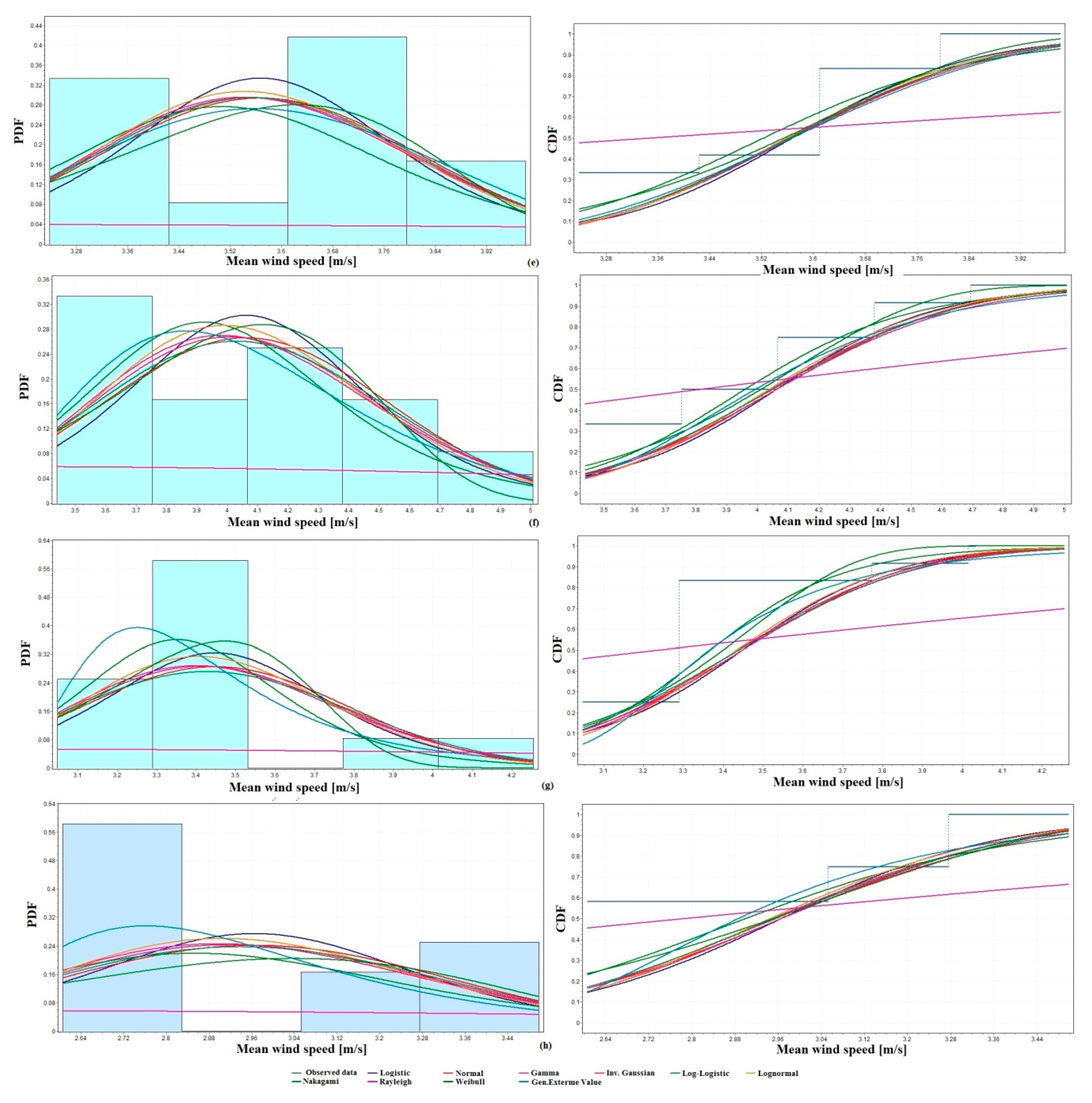
The accuracy of these distributions, characterized by their ability to fit the observed data, has a significant impact on the efficiency and uncertainty of the estimated wind energy productions at a particular site. In the literature, some well-known PDFs and CDFs, including Weibull, Rayleigh, Generalized Extreme Value, Gamma, Normal, Log-normal, Logistic, Log-logistic, and Inverse Gaussian [7,8,9,10,11,12], have been used to model the wind speed and power density distributions. For instance, Ouarda et al. [7] investigated the wind speed characteristics of nine stations in UAE using eleven distribution functions. The maximum likelihood, moments, least-square and L-moments methods were used to calculate the parameters of the distribution functions. The results indicated that 2-parameter Weibull, Kappa distribution, and generalized Gamma distribution generally provided the best fit to the wind speed data at all heights and for all stations. Aries et al. [8] assessed the accuracy of eight probability functions for analyzing the wind speed distribution at four locations in Algeria and four methods were used to calculate the parameters of these functions. They concluded that the Generalized Extreme Value and Gamma distribution are the most appropriate fit to wind speed data at the four sites and the L-moments method is the most accurate for calculating the distribution parameters. Masseran [9] studied the distribution of the wind power density at six stations in Malaysia using Weibull, Gamma, and Inverse Gamma density functions. The maximum likelihood method was used to estimate the parameters of the models. It was found that the Weibull and Gamma PDF was able to provide a good approximation of the observed wind speed data foreach station. Thus, these PDF models were reliable for estimating the wind energy potential in the studied sites.
Electrical energy in Northern Cyprus is produced by fossil fuels and a photovoltaic power plant, which is located in Serhatköy. The power generation in Northern Cyprus is around 212 MW for the diesel generator and 1.27 MW for the photovoltaic power plant, i.e., the total power generation in Northern Cyprus is approximately 300 MW [13,14,15]. Additionally, population growth and other factors in Northern Cyprus have led to an increase in the demand for fossil fuels. As a result, energy sources such as wind and solar energy can be considered as alternative energy resources for generating electricity. It is important to evaluate the wind potential in Northern Cyprus and select the proper distribution function for analyzing the wind speed characteristics. However, the literature shows that there is a lack of studies that have investigated the wind power potential in Northern Cyprus; therefore, significant attention is required to assess the wind energy resources to provide suitable data for estimating the wind power potential.
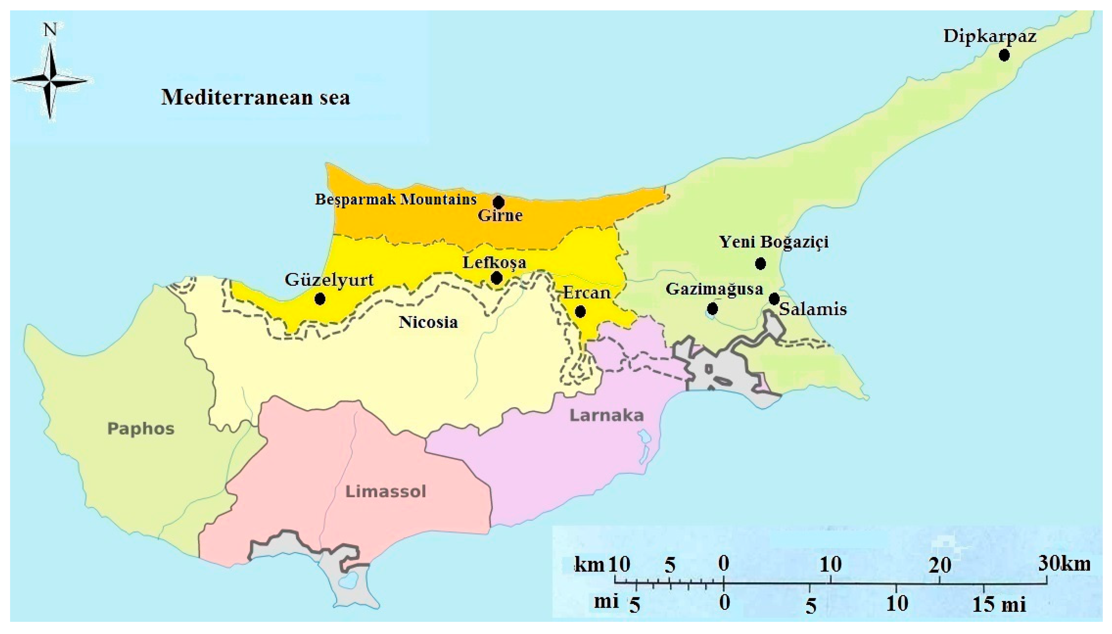
Consequently, the primary goal of this study is to determine the best locations with high potential for wind resources at different locations and to provide suitable data for evaluating the potential wind power output from wind power systems. Thus, this paper aims to analyze the wind speed characteristics in eight regions, namely, Lefkoşa, Ercan, Girne, Güzelyurt, Gazimağusa, Dipkarpaz, Yeni Boğaziçi and Salamis in Northern Cyprus. The data consists of monthly data, annual data, and wind speed direction data. In particular, the analysis of wind speeds for each region was conducted for various periods. Thus, the wind speed data were collected from the Meteorology Department located in Lefkoşa. Ten distribution functions were applied to explore the wind speed characteristics and to determine the wind power potential in each region. The wind power density as a function of hub height is studied in order to classify the wind energy resources in Northern Cyprus. Moreover, a technical and economic assessment has been made for the generation of electricity using vertical axis wind turbines at eight locations. The reasons for choosing a vertical axis wind turbine instead of a horizontal axis wind turbine are: (a) they are good for a low-wind-speed environment; (b) they can be installed in locations with restricted space such as rooftops, buildings or on top of communication towers; and (c) there is no need for a yaw mechanism since they operate independently from the wind direction.
The rest of the paper is structured as follows: Section 2 presents the overall information about the collected wind data, wind data adjustment, and analysis procedure. Section 3 describes the wind speed characteristics at the studied locations and analyzes the wind power densities at different heights to evaluate the wind energy potential in detail. It also discusses the economic evaluation and the performance of small-scale vertical axis wind turbines. Section 4 presents the discussions, and Section 5 provides significant conclusions.

2. Materials and Methods

This section presents the statistical analysis of the wind data measured at a height of 10 m at eight locations in Northern Cyprus. Ten distribution functions are used to determine and evaluate the accuracy of the distribution that best fits the wind speeds of the location. The power law model is utilized to determine the wind speeds at different heights. A technical and economic assessment has been made for the generation of electricity using wind turbines at the studied locations. A flow chart given in Figure 1 is to illustrate the analysis procedure of this study.

2.1. Measurement Data

The wind measurement data that were collected from the Meteorological Department in Lefkoşa, Northern Cyprus, have been analyzed. The data were measured every 1 h by an anemometer at a height of 10 m. The data used for this work are monthly data using a simple statistical method to calculate the average monthly wind speed. The coordinates, records period and characteristics of the selected locations are presented in Table 1. In addition, the detailed geographic information of the selected meteorological stations is illustrated in Figure 2.

2.2. Probability Distribution Functions

Knowledge of wind speed data is required for renewable resource assessment. Several distribution functions are given in the literature to present the wind speed data in selected regions. In this paper, ten probability distribution functions are used to analyze the distributions of wind speed at the selected regions, as shown in Table 2. Furthermore, in the literature, there are various methods available to compute the parameters of the distribution functions, such as the graphical method, the method of moments, and the maximum likelihood method [16]. In this study, the parameter values for each distribution function were calculated using the Maximum likelihood method. Furthermore, the Easy fit and Matlab R2015a software with a CPU- Intel Xeon E5-16XX, 8 core, 64GB ram, and 64-bit Operating System were used in order to obtain the parameters of the distribution functions.

2.3. Wind Power Density

The wind power density (WPD) value can be regarded as a representative value for the wind energy potential of a region. The model of wind power density describes the distributions of wind energy at various wind speed values. The WPD value in W/m2 depends only on the air density and the wind speed as given by [17]
W P D = P A = 1 2 ρ v 3
where P is the wind power in W, A is a swept area in m2, ρ is the air density ( ρ = 1.225 kg / m 3 ) and v is wind speed in m/s.
Moreover, for a period measurement, the mean wind power density ( WPD ¯ ) in W/m2 can be calculated using Equation (2) [18].
WPD ¯ = P ¯ A = 1 2 ρ v ¯ 3
where P ¯ is the mean wind power in W and v ¯ is the mean wind speed in m/s.
If the distribution of wind speed is taken into account, then Equation (1) can be written as [17]
P A = 1 2 ρ 0 v 3 f ( v ) d v
where f ( v ) is the probability density function (PDF).
Furthermore, the wind power density distribution for a specified distribution function f(v) can be computed as [19]
P A = 1 2 ρ v 3 f ( v )
For wind energy assessments, the simple power law model is usually adopted to convert the wind speeds to various heights. It is expressed as [18]
v v 10 = ( z z 10 ) α
where v is the wind speed at the wind turbine hub height z, v 10 is the wind speed at the original height z 10 , and α is the surface roughness coefficient, which depends on the characteristics of the region [13]. In this study, the wind speed data was measured at the height of 10 m above the ground level; therefore, the value of α can be obtained from the following expression [12,18]
α = 0.37 0.088 l n ( v 10 ) 1 0.088 l n ( z 10 / 10 )

2.4. Output Energy of Wind Turbines

The total power output ( E w t ) of the wind turbine can be expressed by Equation (7) [17,20]. In addition, the power curve of the wind turbines can be approximated with a parabolic law, as given by [21] (Equation (8)).
E w t = i = 1 n P w t ( i ) t
where E w t is total power output and t is the number of hours in the period under consideration.
P w t ( i ) = { P r v i 2 v c i 2 v r 2 v c i 2 ( v c i v i v r ) 1 2 ρ A C p v r 2 ( v r v i v c o ) 0   ( v i v c i   a n d   v i v c o )
where v i is the vector of the possible wind speed at a given site, P w t ( i ) is the vector of the corresponding wind turbine output power in W, P r is the rated power of the turbinein W, v c i is the cut-in wind speed (m/s), v r is the rated wind speed (m/s), and v c o is the cut-out wind speed (m/s) of the wind turbine. C p is the coefficient of performance of the turbine, and it is a function of the tip speed ratio and the pitch angle. The coefficient of performance is considered to be constant for the entire range of wind speed [22] and can be calculated as
C p = 2 P r ρ A v r 3
The capacity factor (CF) of a wind turbine is the fraction of the total energy generated by the wind turbine over a period to its potential output if it had operated at a rated capacity during the entire time. The capacity factor of a wind turbine based on the local wind regime of a given site can be estimated as [17]:
C F = E w t P r · t
Several methods have been used to estimate the wind energy cost such as PVC methods [23]. The present value of costs (PVC) is given in Reference [23] as the following equation:
P V C = [ I + C o m r ( 1 + i r i ) × [ 1 ( 1 + i 1 + r ) n ] S ( 1 + i 1 + r ) n ]
where r is the discount rate, i is the inflation rate, n is the machine life as designed by the manufacturer, C o m r is the cost of operation and maintenance, I is the investment summation of the turbine price and other initial costs, including provisions for civil work, land, infrastructure, installation, and grid integration and S is the scrap value of the turbine price and civil work.
The cost per kWh of electricity generated (UCE) can be determined by the following expression [23]:
U C E = P V C t × P r × C F

3. Results

3.1. Description of Wind Speed Data

Table 3 presents the descriptive statistics of each location including the mean velocity, standard deviation, variance coefficient, minimum velocity, median velocity, maximum velocity, Skewness, and Kurtosis. For all locations at a height of 10 m, the mean wind speeds vary from 2.507 m/s to 4.061 m/s. The mean speed and standard deviation values suggest that there is good consistency in the wind behavior. The coefficients of variation are moderately high, ranging from 7.08 to 16.97. During the investigation period, the Skewness value is negative in Lefkoşa, Güzelyurt, and Ercan, which indicates that all distributions are left-skewed. However, the Skewness values of Girne, Gazimağusa, Dipkarpaz, Yeni Boğaziçi, and Salamis are positive, meaning that all distributions are right-skewed. The annual descriptive statistics of wind speed series at the studied locations over various periods to experience different climatic environments are displayed in Table S1 as Supplementary Material.

3.2. Wind Speed Characteristics at a 10m Height

The mean monthly wind speeds for the eight locations are plotted in Figure 3. As can be seen, the mean monthly wind speeds ranged between 1.88 and 5.01 m/s. The minimum and maximum wind speeds occurred in December inLefkoşa and in March in Dipkarpaz, respectively. Dipkarpaz has the maximum mean annual wind speed of 4.06 m/s, followed by Gazimağusa, Ercan, YeniBoğaziçi, and Salamis, as shown in Figure 4. Moreover, it is observed that the mean annual wind speed values in Lefkoşa, Güzelyurt, and Girne are approximately the same, which is about 2.51 m/s.

3.3. Windrose

The wind direction was recorded for each selected location during the investigation periods. A total of 16 directions were considered, and the wind frequencies for these directions are presented in Figure 5. It is observed that the dominant direction of the wind for Lefkoşa and Güzelyurt was found to be west (W) with frequency values of 15.3% and 19.2%, respectively. Additionally, it can be seen that the wind direction with the most significant frequency was west-northwest (WNW) for Girne, Ercan, and Dipkarpaz. For Gazimağusae, the wind direction with the highest rate is south-southwest (SSW). Moreover, the dominant direction of the wind for YeniBoğaziçi and Salamis was found to be north-northwest (NNW) with frequency values of 9.4% and 9.9%, respectively

3.4. Distribution Function Parameters and Wind Power Density at a 10 m Height

The parameters of ten distribution functions were estimated using monthly wind speed data with the maximum likelihood method. The best distribution among the ten distribution functions for each location was evaluated based on the results of the Kolmogorov–Smirnov tests.
The calculated parameters of each distribution function are presented in Table 4 for each selected location along with their mean velocities. Additionally, Figure 6 shows the fitted PDF and CDF models for the observed wind speed data for each location. Furthermore, Table 5 presents the goodness-of-fit statistics in terms of the Kolmogorov–Smirnov tests for each distribution function. Moreover, a distribution with the lowest Kolmogorov–Smirnov value will be selected to be the best model for the wind speed distribution in the studied location [12].
Table 6 presents the ranking of the distribution models for the eight studied locations based on the Kolmogorov–Smirnov tests. Hence, based on the Kolmogorov–Smirnov tests, GEV has the lowest value, which is considered as the best distribution function to study the wind speed characteristics of Lefkoşa, Güzelyurt, Girne, Ercan, and Dipkarpaz and is ranked the overall third best for Gazimağusa and YeniBoğaziçi, while GEV is ranked the fifth best overall for Salamis, as shown in Table 6. Additionally, LL, W, and G are the best distribution for analyzing the wind speeds of Gazimağusa, YeniBoğaziçi, and Salamis, respectively, as shown in Table 5 and Table 6. Moreover, it is observed that the Rayleigh distribution function cannot be used to investigate the wind potential in the studied Location, as shown in Table 6.
Table 7 shows the wind power density values that have been estimated based on the mean actual wind speed and density functions for each location. It is found that the mean actual wind power density (W/m2) is in the range of 9.63 W/m2 and 40.95 W/m2. Dipkarpaz and Gazimağusa have a higher mean wind power density compared with the other locations.
The surface roughness values of the eight selected locations determined using Equation (6) are presented in Table 8. The annual mean wind speed values of these locations at different heights (30, 50, and 90 m) are calculated using the power law method (Equation (5)) and summarized in Table 8. It is observed that as the height above the ground increases, the wind speed also increases. The best wind speed for installing wind turbines should be in the range of 6.7 and 11 m/s according to Mostafaeipour [24]. Therefore, Dipkarpaz is the best locationfor installing wind turbines with a hub height greater than 90 m. In addition, it is observed that at a height of 90 m, the annual mean wind speed in Gazimağusa, Ercan, and YeniBoğaziçi is above 6 m/s.
The 90 m synthesized data for the studied locations is presented in Figure 7. As per the actual data at 10 m, the synthesized data is also matched byusing ten distribution functions. Moreover, Table 9 shows the calculated parameters, mean speed, and wind power density (WPD) of each distribution functions at a height of 90 m. Mean speed and WPD values vary from 4.204 to 7.877 m/s and 45.430 to 298.865 W/m2, respectively. The maximum value of the annual wind power of 298.865 W/m2 is recorded in Gazimağusa, whereas the minimum value of 45.430 W/m2 is obtained in Girne.
Furthermore, Table 10 shows the results of goodness-of-fit and the selected distribution for each location at a height of 90 m. Based on the Kolmogorov–Smirnov tests, GEV function is the highest match for studying the wind speed characteristics at Lefkoşa, Güzelyurt, Girne, Ercan and Dipkarpaz. However, LL, W and G have the best distributions for analyzing the wind speed for Gazimağusa, YeniBoğaziçi and Salamis, respectively.

3.5. Summary oftheEight Selected Locations in Northern Cyprus

In this section, the wind energy potential of the locations is classified according to the average power density values given in Table 11. The wind power densities of the selected locations ranged from 9.7 to 40.88 W/m2 at 10 m, 25.07 to 92.07 W/m2 at 30 m, and 38.99 to 134.29 W/m2 at 50 m. Therefore, the studied locations can be considered to bePower Class 1, which indicates a poor wind energy potential. Commercial wind turbines with high capacities (MWs) are not suitable to be used in all the studied locations. However, the available wind energy potential of the regions can be exploited using small-scale wind turbines.

3.6. Economic Analysis of the Wind Turbine

Based on Section 3.5, five commercially available small vertical axis wind turbines (VAWT) were selected, and the required technical specifications are given in Table 12. In this study, the annual output energy and the capacity factor of the wind turbines for the selected locations were calculated using Equations (7) and (10) and summarized in Table 13 for the Aeolos-V2 5 kW rated model and Table S2 as Supplementary Material for other selected wind turbine models. In addition, the effect of hub height on the annual energy and capacity factor from the chosen wind turbine is shown in Table 13 for the Aeolos-V2 5 kW rated model, while Table S2 as Supplementary Material shows the effect of hub heights on the annual energy and capacity factor of other models. It is observed that the Aeolos-V2 the 5 kW rated model was found to be most efficient with a maximum annual energy and capacity factor corresponding to various hub heights for the Lefkoşa, Güzelyurt, Girne, YeniBoğaziçi, and Salamis locations. For other locations, WS-12/8 kW has the lower capacity factor corresponding to hub heights of 20 and 30 m in comparison to the other chosen wind turbines. Furthermore, Table 13 shows the energy unit cost per kWh based on the PVC method. This cost is computed using Equations (11) and (12). It is observed that the Aeolos-V2 5 kW rated model has the lowest cost value compared to the other selected turbines for the studied locations.

4. Discussion

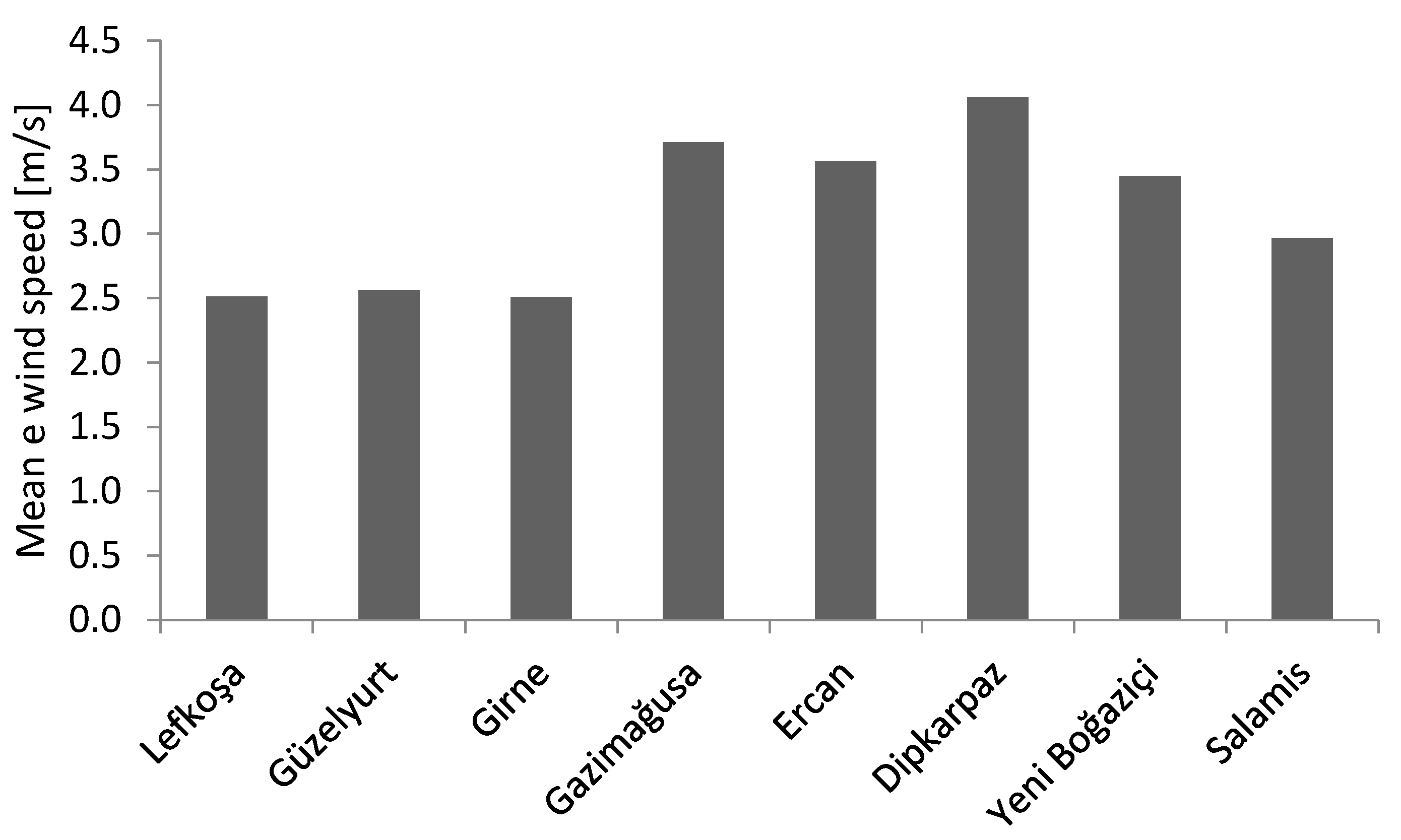
The results show thatthe annual mean wind speeds at all locations in Northern Cyprus are generally higher than 2 m/s at a height of 10 m (Figure 4) and themean monthly wind speed varies within the range of 1.8–5 m/s (Figure 3). Based on Figure 4, the locations (Gazimağusa, Dipkarpaz, YeniBoğaziçi, and Salamis) in the eastern part of Northern Cyprus have higher wind speeds compared to the other locations (Lefkoşa, Girne, and Güzelyurt). In fact, higher wind speeds are mostly seen in the south part of Cyprus and only on the top of the Beşparmak Mountains in the north part of Cyprus [25]. Beşparmak gives its depictive name to the whole mountain range and SelviliTepe in the west with the highest peak of 1024 m are the most renowned and outstanding mountains in North Cyprus. According to Solyali et al. [26], the mean annual wind speed at the Selvili-Tepe location is about 5 m/s at 30 m height. As mentioned previously, there is a lack of studies that have investigated the wind power potential in Northern Cyprus. Therefore, this study is aimed to analyze the wind power potential in different locations in the north part of Cyprus. Thus, the results of the collected data and analysis show that Dipkarpaz has better conditions for developing a wind farm with a wind turbine of 90 m hub height, at which the capacity of the wind turbine is 1 MW or above. The airport (Ercan) is a relatively inappropriatelocatin to install a wind turbine at because this site has a high value of surface roughness, and the turbine will be dangerous to airplanes. Based on the wind power density classes published by the U.S. Department of Energy, the evaluation of the wind resources available in the eight selected locations (which are class 1 wind power site) indicates its suitability for small-scale wind turbine and for off-grid connections (Table 11). From the perspective of the costs of generating electricity, the Aeolos-V2 5 kW model is the most economical option for generating electricity in Northern Cyprus (Table 13 and Table S2).

5. Conclusions

The wind characteristics and wind power potential in several selected locations in Northern Cyprus were discussed. Wind speeds and power density at different heights were estimated using different distribution functions. It is important to note that this step was implemented after the wind analysis at 10 m and after determining the most accurate distribution function. Therefore, it was found that GEV provided the best fit to the actual wind speed data for the regions of Lefkoşa, Güzelyurt, Girne, Ercan, and Dipkarpaz. However, LL, W, and G had the best distribution for analyzing the wind speed of Gazimağusa, YeniBoğaziçi, and Salamis, respectively. All the considered locations have annual mean wind speeds above 2 m/s, and the wind power densities range between 9.59 W/m2 to 40.88 W/m2 at a height of 10 m. Among the eight studied locations, it was observed that Dipkarpaz had the highest winds. The wind power analysis shows that Dipkarpaz is the best location for harvesting wind energy. A techno-economic assessment was made for the generation of electricity using a small-scale vertical axis wind turbine in all the studied locations. It is found that Aeolos-V2 model with a power rating of 5 kW has the lowest energy production cost among the considered wind turbine technologies. Finally, the exploitation of renewable energy sources such as wind energy can help Northern Cyprus achieve many of its environmental and energy policy targets.

Supplementary Materials

The following are available online at https://www.mdpi.com/1996-1073/11/10/2697/s1. Table S1: Annual descriptive statistics of wind speed series at eight-selected Location over various period, Table S2: Annual descriptive statistics of wind speed series at eight-selected Location over various period.

Author Contributions

M.M.A. collected the wind data. Y.K. and H.Ç. analyzed the data and wrote the paper.

Funding

This research received no external funding.

Acknowledgments

The authors would like to thank the Faculty of Engineering especially the Mechanical Engineering Department at Near East University for their support and encouragement.

Conflicts of Interest

The authors declare no conflict of interest.

References

  1. Rasham, A.M. Analysis of Wind Speed Data and Annual Energy Potential at Three locations in Iraq. Int. J. Comput. Appl. 2016, 137, 5–16. [Google Scholar] [CrossRef]
  2. Oyedepo, S.; Adaramola, M.; Paul, S. Analysis of Wind Speed Data and Wind Energy Potential in Three Selected Locations in South-East Nigeria. Wind Resour. Future Energy Secur. 2015, 3–28. [Google Scholar] [CrossRef]
  3. Mostafaeipour, A.; Jadidi, M.; Mohammadi, K.; Sedaghat, A. An analysis of wind energy potential and economic evaluation in Zahedan, Iran. Renew. Sustain. Energy Rev. 2014, 30, 641–650. [Google Scholar] [CrossRef]
  4. Soulouknga, M.; Doka, S.; Revanna, N.; Djongyang, N.; Kofane, T.C. Analysis of wind speed data and wind energy potential in Faya-Largeau, Chad, using Weibull distribution. Renew. Energy 2018, 121, 1–8. [Google Scholar] [CrossRef]
  5. Benatallah, M.; Chegaar, M. Investigation of Wind Characteristics in the Southern Region of Algeria. Energy Procedia 2013, 36, 707–713. [Google Scholar] [CrossRef]
  6. Gökçek, M.; Bayülken, A.; Bekdemir, Ş. Investigation of wind characteristics and wind energy potential in Kirklareli, Turkey. Renew. Energy 2007, 32, 1739–1752. [Google Scholar] [CrossRef]
  7. Bilir, L.; İmir, M.; Devrim, Y.; Albostan, A. An investigation on wind energy potential and small-scale wind turbine performance at İncek region—Ankara, Turkey. Energy Convers. Manag. 2015, 103, 910–923. [Google Scholar] [CrossRef]
  8. Ammari, H.D.; Al-Rwashdeh, S.S.; Al-Najideen, M.I. Evaluation of wind energy potential and electricity generation at five locations in Jordan. Sustain. Cities Soc. 2015, 15, 135–143. [Google Scholar] [CrossRef]
  9. Baseer, M.; Meyer, J.; Alam, M.M.; Rehman, S. Wind speed and power characteristics for Jubail industrial city, Saudi Arabia. Renew. Sustain. Energy Rev. 2015, 52, 1193–1204. [Google Scholar] [CrossRef] [Green Version]
  10. Al Zohbi, G.; Hendrick, P.; Bouillard, P. Wind characteristics and wind energy potential analysis in five sites in Lebanon. Int. J. Hydrog. Energy 2015, 40, 15311–15319. [Google Scholar] [CrossRef]
  11. Dabbaghiyan, A.; Fazelpour, F.; Abnavi, M.D.; Rosen, M.A. Evaluation of wind energy potential in province of Bushehr, Iran. Renew. Sustain. Energy Rev. 2016, 55, 455–466. [Google Scholar] [CrossRef]
  12. Masseran, N. Evaluating wind power density models and their statistical properties. Energy 2015, 84, 533–541. [Google Scholar] [CrossRef]
  13. Ozay, C.; Celiktas, M.S. Statistical analysis of wind speed using two-parameter Weibull distribution in Alaçatı region. Energy Convers. Manag. 2016, 121, 49–54. [Google Scholar] [CrossRef]
  14. Ouarda, T.; Charron, C.; Shin, J.; Marpu, P.; Al-Mandoos, A.; Al-Tamimi, M.; Hosary, T.A. Probability distributions of wind speed in the UAE. Energy Convers. Manag. 2015, 93, 414–434. [Google Scholar] [CrossRef]
  15. Aries, N.; Boudia, S.M.; Ounis, H. Deep assessment of wind speed distribution models: A case study of four sites in Algeria. Energy Convers. Manag. 2018, 155, 78–90. [Google Scholar] [CrossRef]
  16. Allouhi, A.; Zamzoum, O.; Islam, M.; Saidur, R.; Kousksou, T.; Jamil, A.; Derouich, A. Evaluation of wind energy potential in Morocco’s coastal regions. Renew. Sustain. Energy Rev. 2017, 72, 311–324. [Google Scholar] [CrossRef]
  17. Ayodele, T.R.; Jimoh, A.A.; Munda, J.L.; Agee, J.T. Viability and economic analysis of wind energy resource for power generation in Johannesburg, South Africa. Int. J. Sustain. Energy 2013, 33, 284–303. [Google Scholar] [CrossRef]
  18. Irwanto, M.; Gomesh, N.; Mamat, M.; Yusoff, Y. Assessment of wind power generation potential in Perlis, Malaysia. Renew. Sustain. Energy Rev. 2014, 38, 296–308. [Google Scholar] [CrossRef]
  19. Mohammadi, K.; Alavi, O.; Mcgowan, J.G. Use of Birnbaum-Saunders distribution for estimating wind speed and wind power probability distributions: A review. Energy Convers. Manag. 2017, 143, 109–122. [Google Scholar] [CrossRef]
  20. Gökçek, M.; Genç, M.S. Evaluation of electricity generation and energy cost of wind energy conversion systems (WECSs) in Central Turkey. Appl. Energy 2009, 86, 2731–2739. [Google Scholar] [CrossRef]
  21. Pallabazzer, R. Parametric analysis of wind siting efficiency. J. Wind Eng. Ind. Aerodyn. 2003, 91, 1329–1352. [Google Scholar] [CrossRef]
  22. Nouni, M.; Mullick, S.; Kandpal, T. Techno-economics of small wind electric generator projects for decentralized power supply in India. Energy Policy 2007, 35, 2491–2506. [Google Scholar] [CrossRef]
  23. Adaramola, M.; Paul, S.; Oyedepo, S. Assessment of electricity generation and energy cost of wind energy conversion systems in north-central Nigeria. Energy Convers. Manag. 2011, 52, 3363–3368. [Google Scholar] [CrossRef]
  24. Mostafaeipour, A. Feasibility study of harnessing wind energy for turbine installation in province of Yazd in Iran. Renew. Sustain. Energy Rev. 2010, 14, 93–111. [Google Scholar] [CrossRef]
  25. Maxoulis, C.N.; Kalogirou, S.A. Cyprus energy policy: The road to the 2006 world renewable energy congress trophy. Renew. Energy 2008, 33, 355–365. [Google Scholar] [CrossRef]
  26. Solyali, D.; Altunç, M.; Tolun, S.; Aslan, Z. Wind resource assessment of Northern Cyprus. Renew. Sustain. Energy Rev. 2016, 55, 180–187. [Google Scholar] [CrossRef]
Figure 1. The flowchart of the analysis procedure of the present study.
Energies 11 02697 g001
Figure 2. The geographic location of the study area.
Energies 11 02697 g002
Figure 3. The mean monthly wind speed at the eight selected locations during the studied periods.
Energies 11 02697 g003
Figure 4. The mean annual wind speed at the eight selected locations during the studied periods.
Energies 11 02697 g004
Figure 5. The windrose diagram during the studied periods; (a) Lefkoşa, (b) Güzelyurt, (c) Girne, (d) Gazimağusa, (e) Ercan, (f) Dipkarpaz, (g) YeniBoğaziçi, and (h) Salamis.
Energies 11 02697 g005
Figure 6. Fitting the probability density function (PDF) and cumulative distribution function (CDF) models to the wind speed data at a height of 10 m (a) Lefkoşa, (b) Güzelyurt, (c) Girne, (d) Gazimağusa, (e) Ercan, (f) Dipkarpaz, (g) YeniBoğaziçi, and (h) Salamis.
Energies 11 02697 g006aEnergies 11 02697 g006b
Figure 7. Fitting PDF and CDF models to the wind speed data at a height of 90 m (a) Lefkoşa, (b) Güzelyurt, (c) Girne, (d) Gazimağusa, (e) Ercan, (f) Dipkarpaz, (g) YeniBoğaziçi, and (h) Salamis.
Energies 11 02697 g007aEnergies 11 02697 g007b
Table 1. The details of each location used in this study.
LocationCoordinatesPeriod RecordsYearCharacteristics of the Location
Latitude (°N)Longitude (°E)
Lefkoşa35°11′8.0376″33°22′56.1936″2008–20169Surrounded by building
Ercan35°9′31.5828″33°30′14.364″2000–201617Airport
Girne35°19′26.328″33°18′50.274″2000–201617Coastal
Güzelyurt35°12′44.3412″32°58′39.2412″2000–201617Coastal
Gazimağusa35°6′53.6832″33°55′9.282″2000–201617Coastal
Dipkarpaz35°37′3.6552″34°24′31.4316″2005–201612Coastal
YeniBoğaziçi35°19′0.3864″33°57′14.7492″2011–20166Coastal
Salamis35°12′20.5056″33°53′56.5584″2009–20168Coastal
Table 2. The expressions of the statistical distributions used in this study [12,14,15,16].
Distribution FunctionPDFCDF
Weibull (W) P D F = ( k c ) ( v c ) k 1 e x p ( ( v c ) k ) C D F = 1 e x p ( ( v c ) k )
Gamma (G) P D F = v β 1 α β Γ ( β ) e x p ( v β ) C D F = γ ( β , v α ) Γ ( β )
Lognormal (LN) P D F = 1 v σ 2 π e x p [ 1 2 ( l n ( v ) μ σ ) 2 ] C D F = 1 2 + e r f [ l n ( v ) μ σ 2 ]
Logistic (L) P D F = e x p ( v μ σ ) σ { 1 + e x p ( v μ σ ) } 2 C D F = 1 1 + e x p ( v μ σ )
Log-Logistic (LL) P D F = ( ( β α ( v α ) β 1 ) ( 1 + v α ) β ) 2 C D F = 1 ( 1 + v α ) β
Inverse Gaussian (IG) P D F = ( λ 2 π v 2 ) 1 2 e [ λ ( v μ ) 2 2 μ 2 v ] C D F = Φ ( λ v ( v μ 1 ) ) + e x p ( 2 λ μ ) Φ ( λ v ( v μ + 1 ) )
Generalized Extreme Value (GEV) P D F = 1 α [ 1 ζ ( v ) μ α ] 1 ζ 1 e x p [ ( 1 1 ζ ( v ) μ α ) 1 ζ ] C D F = e x p [ ( 1 1 ζ ( v ) μ α ) 1 ζ ]
Nakagami (Na) P D F = 2 m m Γ ( m ) Ω m v 2 m 1 e ( m Ω G 2 ) C D F = γ ( m , m Ω v 2 ) Γ ( m )
Normal (N) P D F = 1 2 π σ 2 e x p ( v μ 2 σ 2 ) C D F = 1 2 [ 1 + e r f ( v μ σ 2 ) ]
Rayleigh (R) P D F = 2 v c 2 e ( v c ) 2 C D F = 1 e x p [ ( v c ) 2 ]
WkShape parameterLL β Shape parameterNa m Shape parameter
c, m/sScale parameter α Scale parameter Ω Scale parameter
G β Shape parameterIG λ Shape parameterN σ Standard deviation
α Scale parameter μ Mean parameter μ Mean parameter
LN σ Shape parameterGEV μ Location ParameterRc, m/sScale parameter
μ Scale parameter ζ Scale parameter
L μ Location Parameter α Shape parameter
σ Scale Parameter
Table 3. The annual descriptive statistics of wind speed series at the eight-selected locationsduring the investigation period.
LocationMeanStandard DeviationVariation CoefficientMinimumMedianMaximumSkewnessKurtosis
(m/s)(m/s)(m/s)(m/s)
Lefkoşa2.5130.42616.971.8822.5673.203−0.08−1.01
Güzelyurt2.5610.2419.392.1192.6472.869−0.63−0.61
Girne2.5070.26410.522.1512.4512.950.39−1.1
Gazimağusa3.7110.3148.473.4053.5114.1420.54−1.8
Ercan3.5670.2537.083.2383.6473.981−0.02−1.36
Dipkarpaz4.0610.4711.583.4384.0525.0060.57−0.22
Yeni-Boğaziçi3.4480.3389.83.0483.4034.2551.352.15
Salamis2.9650.35311.922.6062.7883.4980.52−1.55
Table 4. The parameter values of the different distribution functions over the investigated period at a 10 m height.
Distribution FunctionsActual MeanLefkoşaGüzelyurtGirneGazimağusaErcanDipkarpazYeni BoğaziçiSalamis
2.5132.5612.5073.7113.5674.0613.4482.965
GMean2.5132.562.5073.7113.5674.0633.4472.967
Variance0.170.0610.0630.0890.0590.1970.0980.121
β37.084108.25899.632155.376216.20983.567121.18972.68
α0.0680.0240.0250.0240.0160.0490.0280.041
GEVMean2.5122.5782.5034.8113.5664.0593.448Inf
Variance0.1610.0960.064Inf0.0570.2080.117Inf
ζ−0.417−1.061−0.0680.913−0.401−0.0390.121.23
α0.4250.3010.2150.120.2510.3730.2220.117
μ2.3962.5862.3933.4913.4953.8573.292.686
IGMean2.5132.562.5073.7113.5674.0633.4472.967
Variance0.1760.0620.0630.0880.0590.1970.0960.12
μ2.5132.562.5073.7113.5674.0633.4472.967
λ90.059269.797250.013580.898767.167340.758427.296216.968
LMean2.5212.5822.4933.6833.5724.0353.4052.937
Variance0.1990.0670.0770.1160.0730.2290.0940.159
μ2.5212.5822.4933.6833.5724.0353.4052.937
σ0.2460.1430.1530.1870.1490.2640.1690.22
LLMean2.5412.5892.53.6883.5764.053.4132.945
Variance0.2210.0730.0770.1120.0750.2290.090.155
β0.9160.9460.911.3011.2711.3921.2241.071
α0.10.0570.0610.050.0420.0650.0480.073
LNMean2.5172.5612.5083.7123.5674.0643.4482.968
Variance0.1940.0680.0690.0960.0650.2150.1050.132
σ0.9080.9350.9141.3081.2691.3961.2331.081
μ0.1730.1020.1040.0830.0710.1140.0940.122
NaMean2.5132.5612.5073.7113.5674.0613.4482.965
Variance0.1680.0590.0630.0890.0590.1990.1010.123
m9.53927.9725.06238.6554.4820.80429.48618.059
Ω6.486.6166.34813.86312.78116.69311.9928.915
NMean2.5132.562.5073.7113.5674.0633.4472.967
Variance0.180.0630.070.0990.0640.2210.1140.136
μ2.5132.562.5073.7113.5674.0633.4472.967
σ0.4250.2520.2640.3140.2530.470.3370.369
RMean2.2562.2792.2333.2993.1683.6223.0682.648
Variance1.3911.4191.3622.9752.7433.5852.5721.915
c1.81.8181.7822.6332.5282.892.4482.113
WMean2.5152.5652.5023.7063.5654.0473.4232.963
Variance0.1740.0530.0820.1190.0690.2790.1810.154
c2.6872.6652.6243.8553.684.273.6033.129
k7.09713.55310.53713.10316.6719.1699.6639.029
Inf: Infinity.
Table 5. The results of the goodness-of-fit and the selected distribution (in bold) for each location.
ModelLefkoşaGüzelyurtGirneGazimağusaErcanDipkarpazYeni BoğaziçiSalamis
Kolmogorov–SmirnovStatistic
G0.14140.22740.15320.31010.18630.12900.24600.2066
GEV0.12890.13950.11760.27850.17140.11180.20050.2556
IG0.15070.21450.16730.32130.17690.14400.25900.2723
L0.16220.23300.17720.33820.19000.15350.24840.2875
LL0.18920.24360.12850.24140.23180.13970.19790.2313
LN0.15040.23370.15220.32090.19380.14380.23430.2627
Na0.13920.22610.15650.30810.18330.12670.25200.2554
N0.14000.21660.16630.31570.17770.13670.25830.2670
R0.35650.41600.43910.48370.47640.43050.45870.4548
W0.15090.20940.14210.26020.19210.13250.16910.2360
Table 6. The ranking of the distribution functions for all locations at a height of 10 m based on the goodness-of-fit statistics.
StatisticLocationRank of the Distribution Function
12345678910
Kolmogorov–SmirnovLefkoşaGEVNaNGLNIGWLLLR
GüzelyurtGEVWIGNNaGLNLLLR
GirneGEVLLWLNGNaNaIGLR
GazimağusaLLWGEVNaGNLNIGLR
ErcanGEVIGNNaGLWLNLLR
DipkarpazGEVNaGWNLLLNIGLR
YeniBoğaziçiWLLGEVLNGLNaNIGR
SalamisGLLWNaGEVLNNIGLR
Table 7. The mean wind power density (W/m2) of all selected locations at a height of 10 m.
ModelLefkoşaGüzelyurtGirneGazimağusaErcanDipkarpazYeni BoğaziçiSalamis
Actual9.7010.279.6331.2527.7540.9525.0615.94
G9.7110.269.6331.2527.7541.0025.0415.97
GEV9.7010.489.5968.0927.7240.8825.06-
GI9.7110.269.6331.2527.7541.0025.0415.97
L9.8010.539.4730.5527.8640.1824.1415.49
LL10.0410.619.5530.6727.9740.6124.3115.62
LN9.7510.289.6431.2727.7641.0625.0615.99
Na9.7010.279.6331.2627.7540.9625.0715.94
N9.7110.269.6331.2527.7541.0025.0415.97
R7.027.246.8121.9619.4529.0617.6611.35
W9.7310.329.5831.1227.7040.5424.5215.91
Table 8. The roughness values (α) and mean wind speed at various heights of the studied locations.
LocationLefkoşaGüzelyurtGirneGazimağusaErcanDipkarpazYeni BoğaziçiSalamis
α0.2900.2880.2900.2550.2580.2470.2610.275
Mean (m/s] at 10 m2.5132.5612.5073.7113.5674.0613.4482.965
Mean (m/s] at 30 m3.4473.5103.4434.9084.7355.3224.5914.005
Mean (m/s] at 50 m3.9944.0643.9905.5895.4026.0365.2464.607
Mean (m/s] at 90 m4.7314.8114.7286.4906.2876.9766.1155.412
Table 9. Distribution parameters and wind power density at 90 m.
Distribution functionValueLefkoşaGüzelyurtGirneGazimağusaErcanDipkarpazYeni BoğaziçiSalamis
Actual mean4.7534.8184.7366.4976.2926.9916.1245.425
ActualWPD65.66968.40364.971167.721152.297208.899140.42597.618
GMean4.7324.8114.7296.4916.2866.9786.1155.412
Variance0.3980.140.1340.1620.1180.3790.20.262
β56.278165.493166.816260.407335.768128.501187.288111.84
α0.0840.0290.0280.0250.0190.0540.0330.048
WPD64.7868.08664.68167.219151.874207.728139.82596.915
GEVMean4.7314.724.7247.8776.2846.9716.116Inf
Variance0.3810.3630.131Inf0.1130.390.23Inf
ζ−0.437−1.074−0.1360.903−0.404−0.0620.1011.144
α0.6580.5820.3270.1730.3550.5240.3210.185
μ4.5594.7384.5756.1916.1856.6995.8955.005
WPD64.73764.28964.48298.865151.769207.18139.883-
IGMean4.7324.8114.7296.4916.2866.9786.1155.412
Variance0.4080.1430.1340.1610.1180.3770.1960.26
μ4.7324.8114.7296.4916.2866.9786.1155.412
λ259.944779.785790.291701.412103.12900.3251167.69609.158
WPD64.7868.08664.68167.219151.874207.728139.82596.915
LMean4.7454.8464.7116.4546.2936.9436.0585.369
Variance0.4670.1560.160.2070.1460.440.1910.342
μ4.7454.8464.7116.4546.2936.9436.0585.369
σ0.3770.2180.220.2510.2110.3660.2410.322
WPD65.3369.57863.937164.406152.403204.693135.93394.616
LLMean4.774.8544.7196.466.2986.9596.0675.379
Variance0.5040.1660.1590.2020.1490.4390.1830.334
β1.5521.5761.5481.8631.8381.9361.81.677
α0.0810.0460.0460.0380.0340.0520.0390.059
WPD66.3769.9364.274164.831152.771206.107136.57195.16
LNMean4.7364.8124.736.4926.2876.986.1165.414
Variance0.4470.1560.1450.1740.1290.4120.2140.284
σ1.5451.5681.5511.8681.8371.9391.8081.684
μ0.140.0820.080.0640.0570.0920.0750.098
WPD64.96468.15464.725167.29151.937207.926139.89997.018
NaMean4.7314.8114.7296.4916.2866.9786.1155.412
Variance0.3910.1370.1350.1630.1170.3820.2040.264
m14.43142.25841.65964.73684.28132.00845.88827.847
Ω22.77823.27922.50142.29539.62949.07237.60329.554
WPD64.7768.07764.685167.229151.874207.76139.85696.934
NMean4.7324.8114.7296.4916.2866.9786.1155.412
Variance0.4240.1480.1470.1780.1280.4220.2290.292
μ4.7324.8114.7296.4916.2866.9786.1155.412
σ0.6510.3840.3830.4220.3580.6490.4780.541
WPD64.7868.08664.68167.219151.874207.728139.82596.915
RMean4.234.2764.2045.7645.5796.2085.4344.818
Variance4.8884.9964.8299.0778.50410.5318.076.342
c3.3753.4123.3544.5994.4514.9534.3363.844
WPD46.26947.80745.43117.074106.182146.31398.14468.385
WMean4.7334.8194.7196.4816.2826.9546.0775.405
Variance0.4190.1250.1830.2260.1410.5480.3810.342
c5.0054.9734.9046.6896.4477.2716.3425.655
k8.73116.78513.48416.80420.7311.37511.9611.189
WPD64.82368.43364.267166.48151.608205.599137.23896.548
Inf: Infinity.
Table 10. Results of goodness-of-fit and the selected distribution (in bold) for each location at 90 m.
ModelLefkoşaGüzelyurtGirneGazimağusaErcanDipkarpazYeni BoğaziçiSalamis
Kolmogorov–Smirnov statistic
G0.14160.22750.15250.31040.18690.13000.24460.2207
GEV0.12830.13920.11770.27770.17170.11200.19980.3467
IG0.14460.21700.16380.31940.17930.14190.25500.3003
L0.15840.23540.17360.33750.19250.15390.24400.2852
LL0.18920.24360.12850.24140.23180.13970.19790.2313
LN0.15040.23370.15220.32090.19380.14380.23430.2627
Na0.14030.22670.15530.30890.18450.12550.24990.2555
N0.13630.21880.16310.31500.18000.13250.25440.2649
R0.39040.43980.45910.49550.48950.45200.47510.4722
W0.15090.20940.14210.26020.19210.13250.16910.2360
Table 11. The summary ofthe eight selected locations in Northern Cyprus.
VariableLefkoşaGüzelyurtGirneGazimağusaErcanDipkarpazYeni BoğaziçiSalamis
Value
The power density at 10 m (W/m2)9.710.489.5930.6727.7240.8824.5215.97
The power density at 30 m (W/m2)25.0726.1024.8971.1664.9892.0758.1239.35
The power density at 50 m (W/m2)38.9941.2838.76105.1696.49134.2986.7259.88
Wind power class1 (poor)
Surface roughness0.2900.2880.290.2550.2580.2470.2610.275
Mean at 90 m(m/s)4.734.814.736.496.296.986.115.41
Table 12. The vertical axis small wind turbine specifications.
ModelRated Power (kW)Rated Wind Speed (m/s)Cut-in Wind Speed (m/s)Rotor Diameter (m)Rotor Height (m)
WRE.030/3 kW31423.32.2
Aeolos-V2 5 kW5102.54.25.3
WRE.060/6 kW61423.34.4
WS-12/8 kW820226
Aeolos-V 10 kW10122.54.25.3
Table 13. The electricity production and financial indices atthe eight locations for the Aeolos-V2 5 kW model at various hub heights.
LocationHub Height (m)Total Energy Power of Wind Turbine (kW)CF (%)UCE ($/kW)
Lefkoşa2043.1835.980.61
3075.8363.190.35
40104.1386.770.25
Güzelyurt2052.4443.70.51
3093.9178.260.28
40129.85108.210.20
Girne2053.6344.690.49
3095.4279.520.28
40131.631000.20
Gazimağusa20296.231000.09
30402.341000.07
40494.281000.05
Ercan20247.461000.11
30340.641000.08
40421.381000.06
Dipkarpaz20308.531000.09
30417.91000.06
40512.671000.05
Yeni Boğaziçi20103.6986.410.26
30146.031000.18
40182.71152.260.15
Salamis2084.2270.180.31
30125.631000.21
40161.521000.16

