Modeling and Enhanced Error-Free Current Control Strategy for Inverter with Virtual Resistor Damping


Abstract
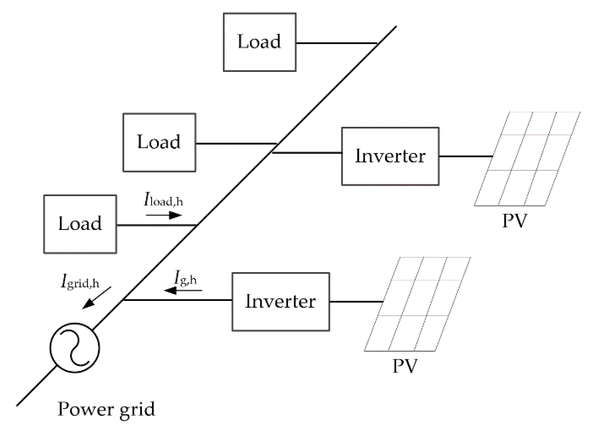
:1. Introduction
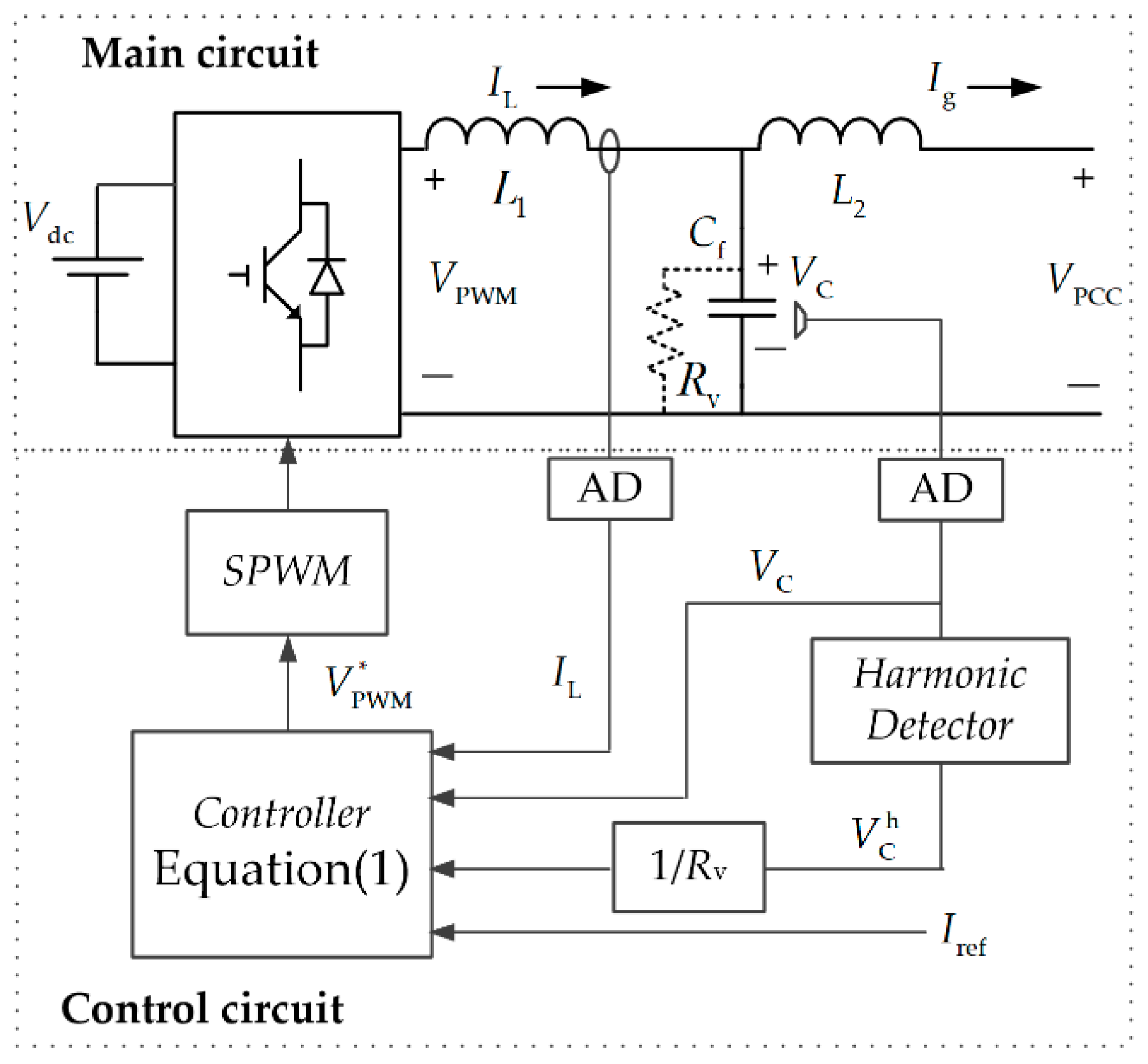
2. Modelling of the Inverter with Virtual Resistor Control
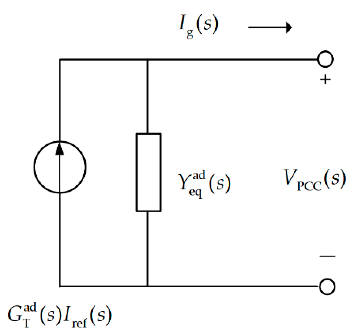
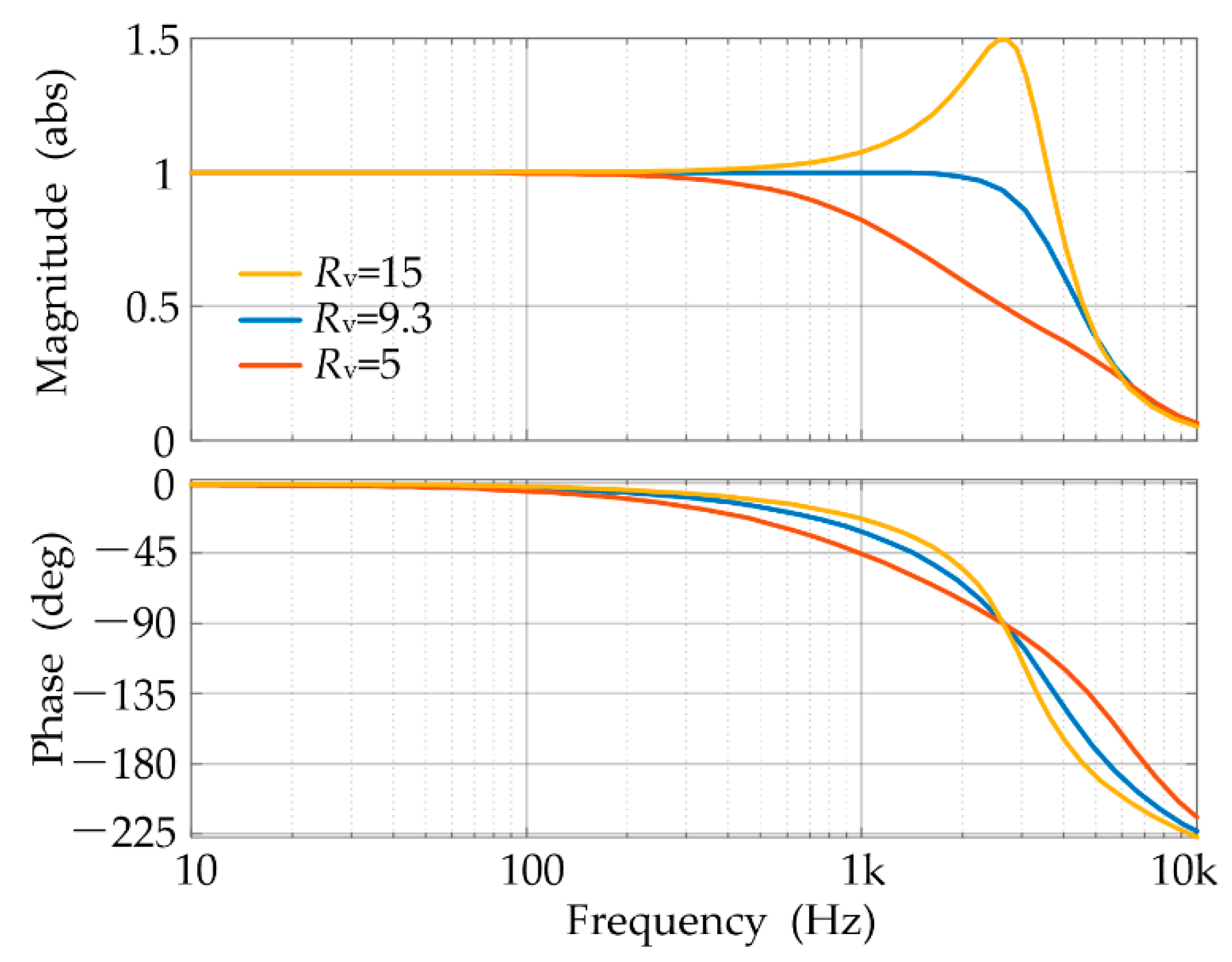
3. Optimal Virtual Resistor Value of the Inverter
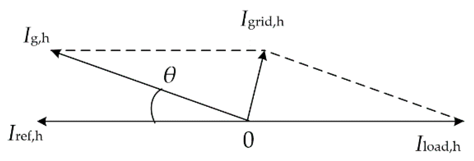
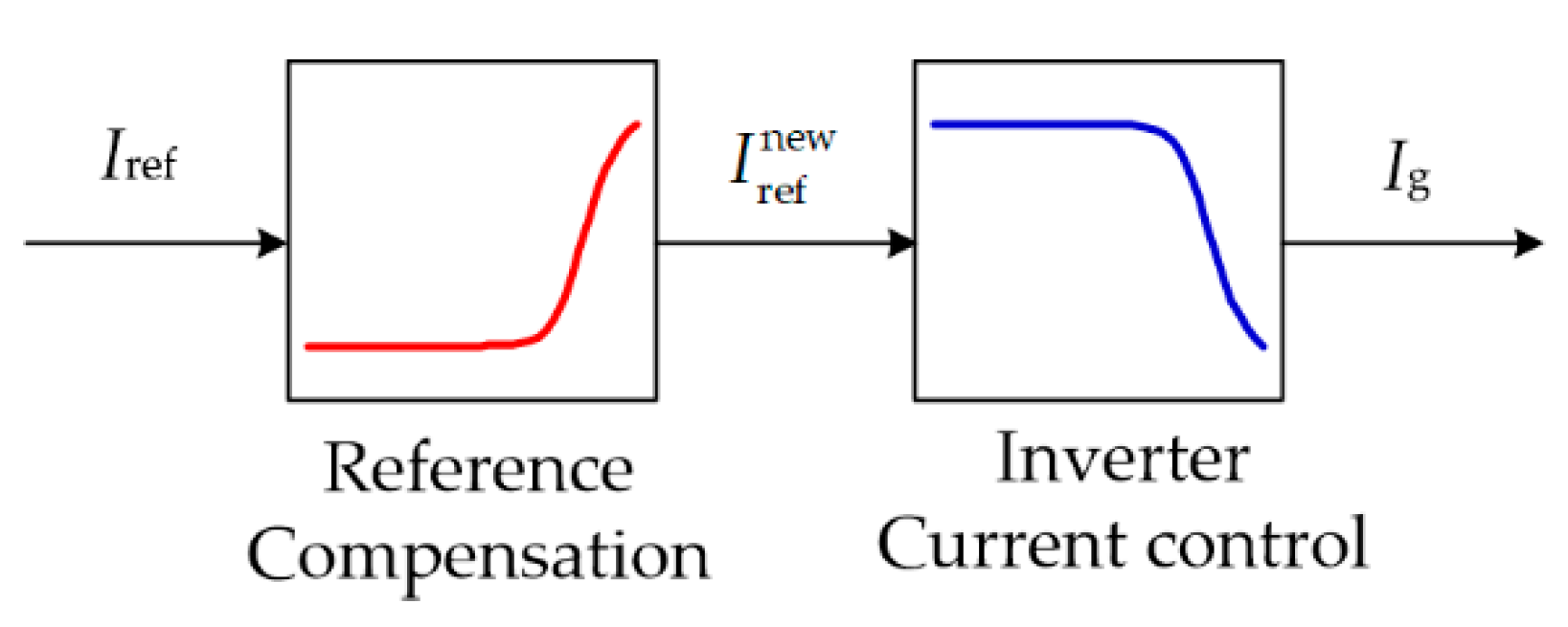
4. Reference Current Compensation Method
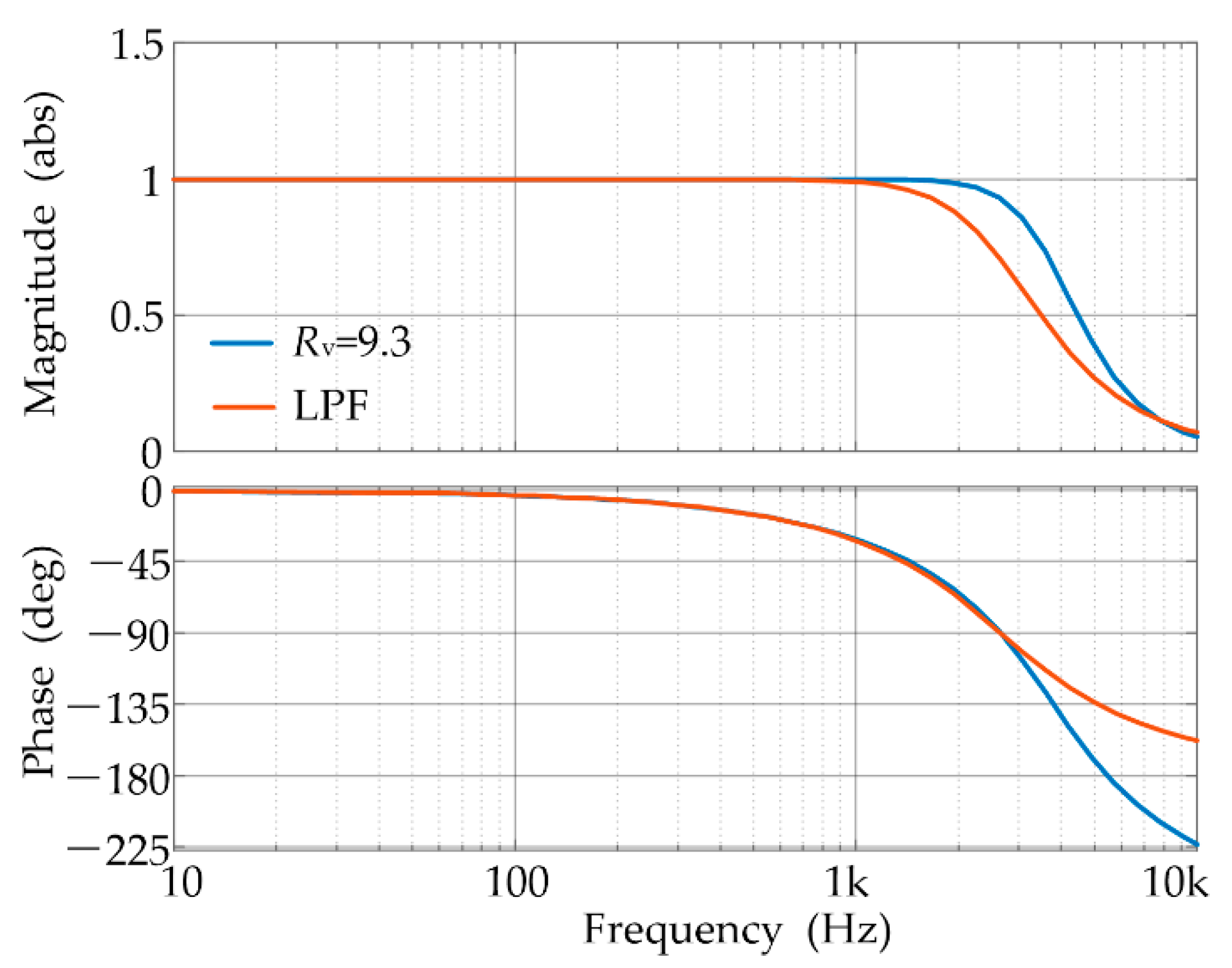
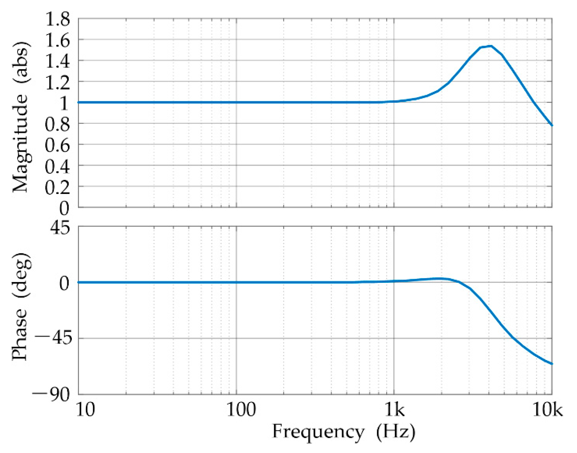
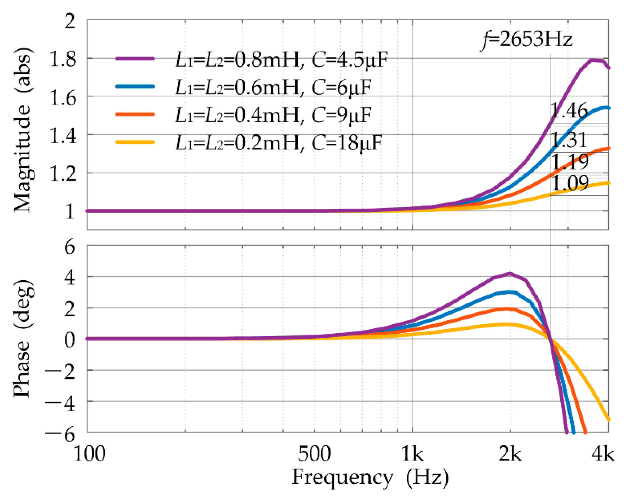
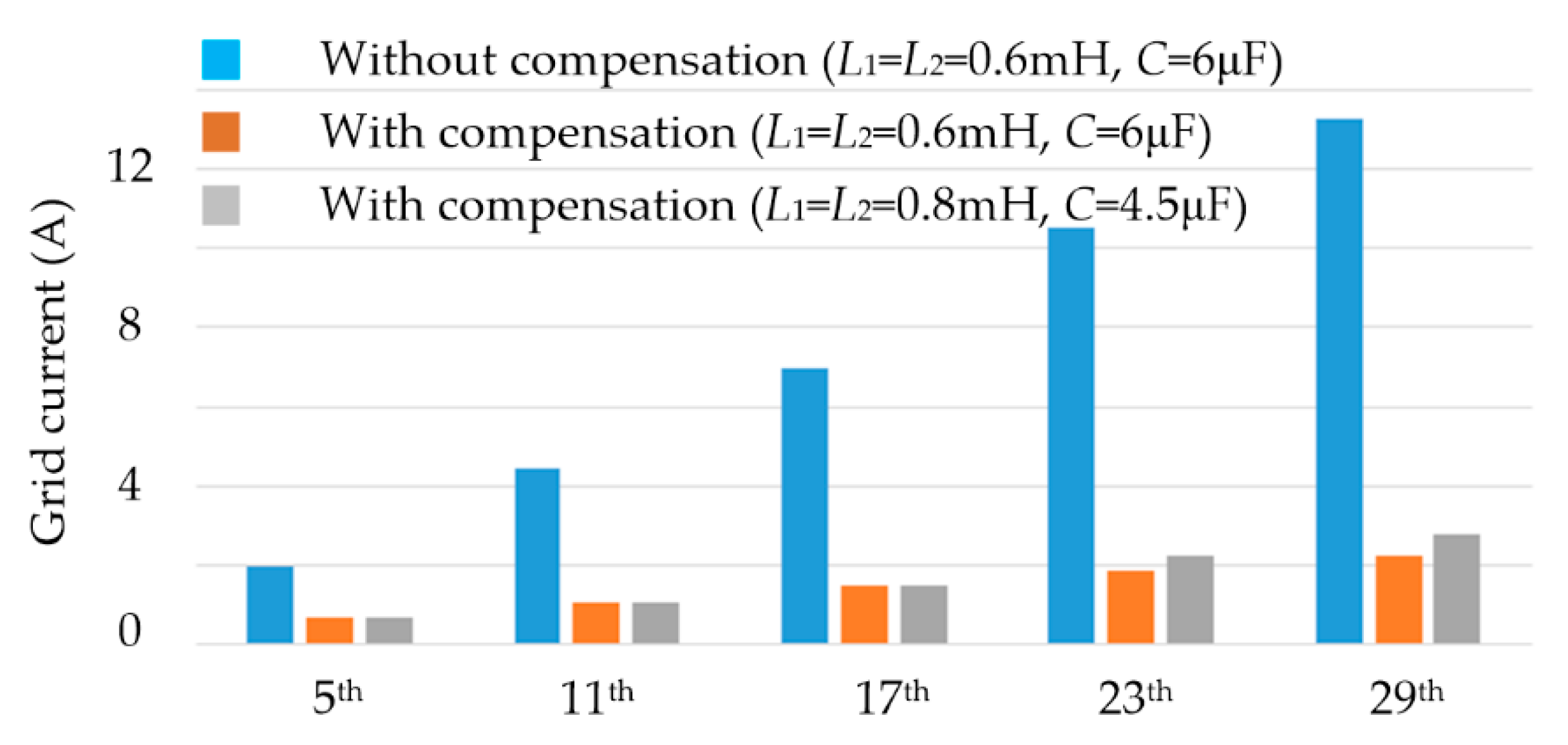
5. Effect of LCL Parameters on Performance of the Reference Compensation Method
- Below cut-off frequency, the higher the inductance value, the greater the overshoot of the amplitude-frequency curve; Conversely, the lower the inductance value, the amplitude-frequency curve is closer to unit 1.
- Below cut-off frequency, the higher the inductance value, the greater the overshoot of the phase-frequency curve; Conversely, the lower the inductance value, the phase-frequency curve is closer to zero.
6. Simulation and Experimental Verification
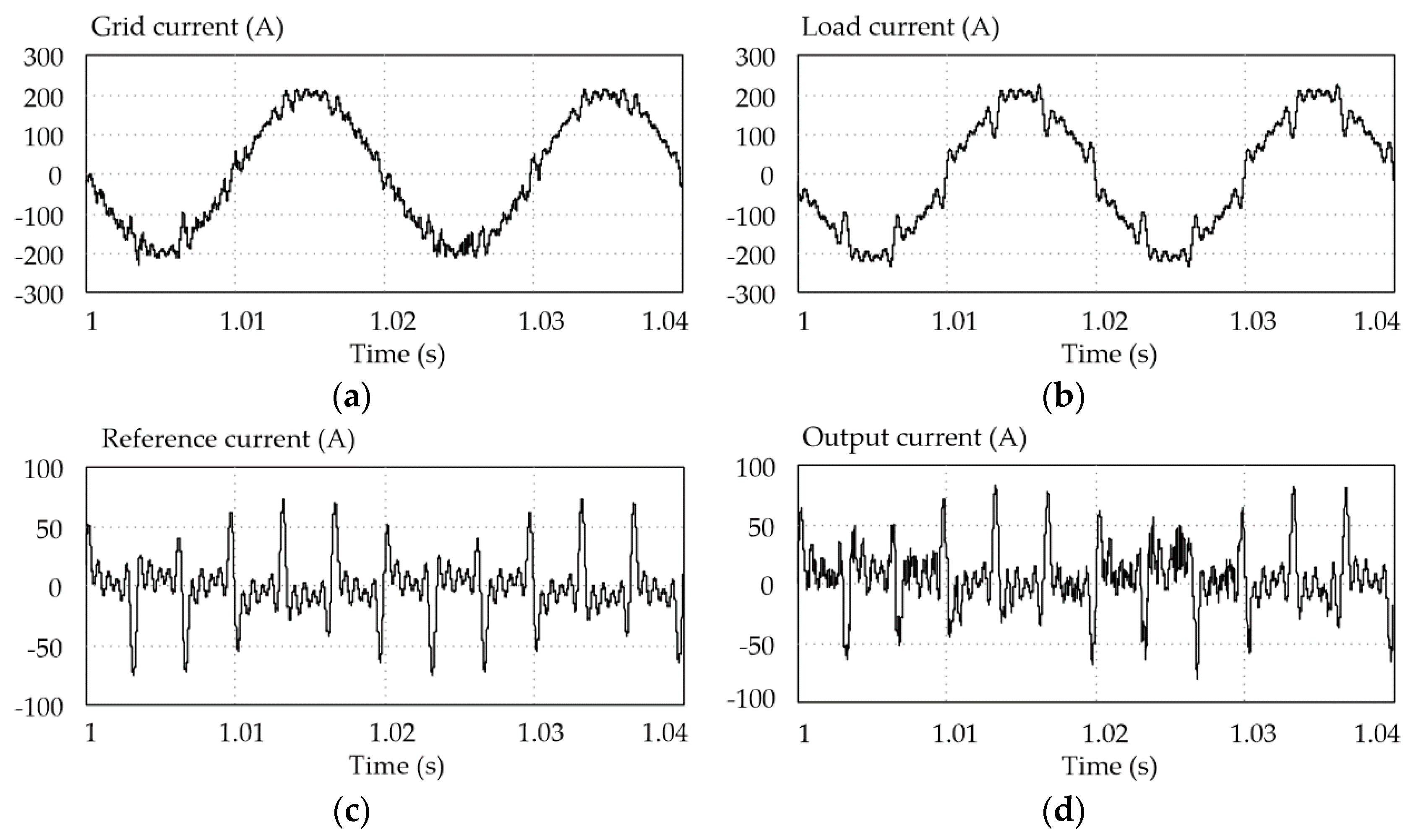
6.1. Simulation
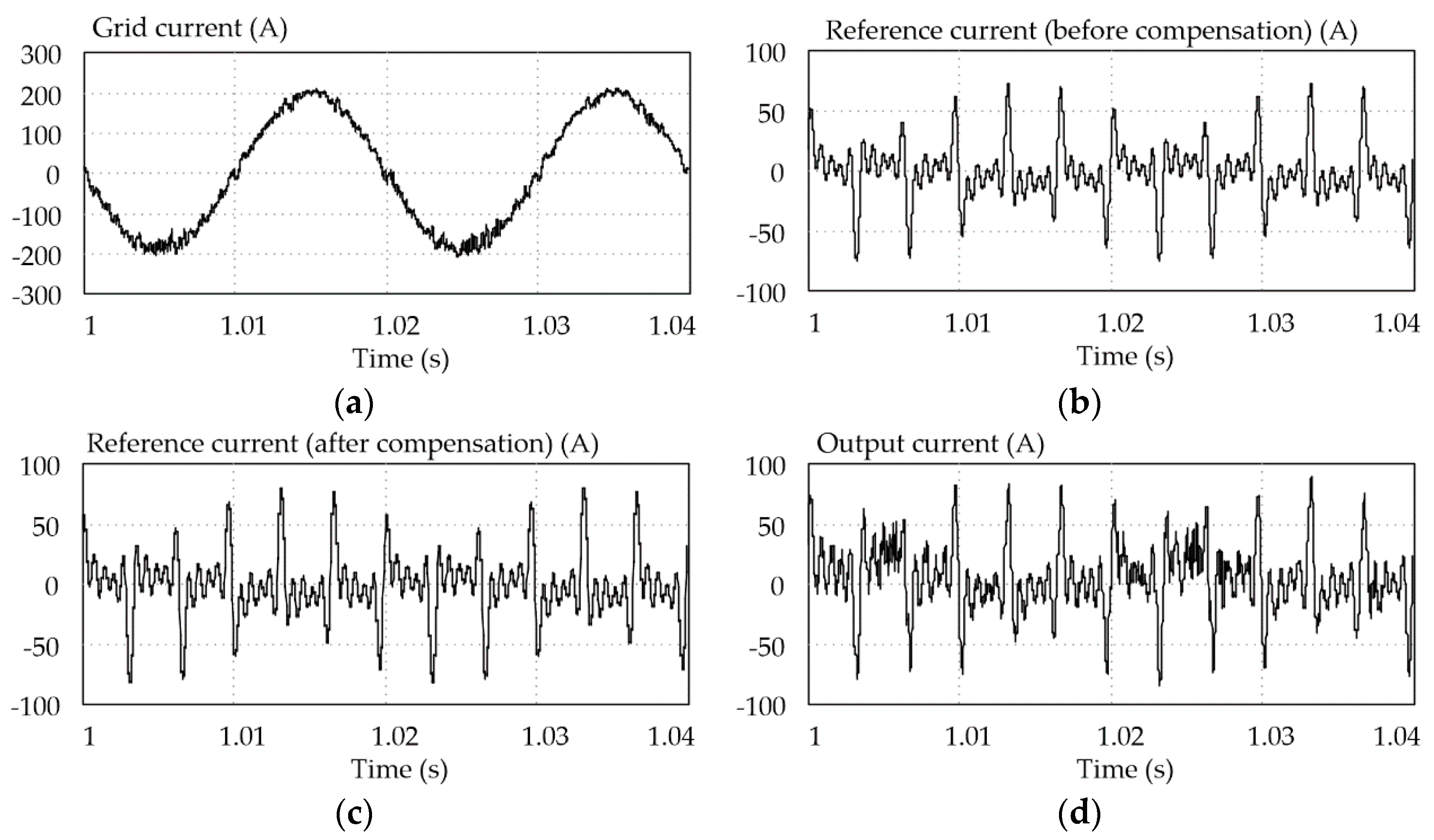
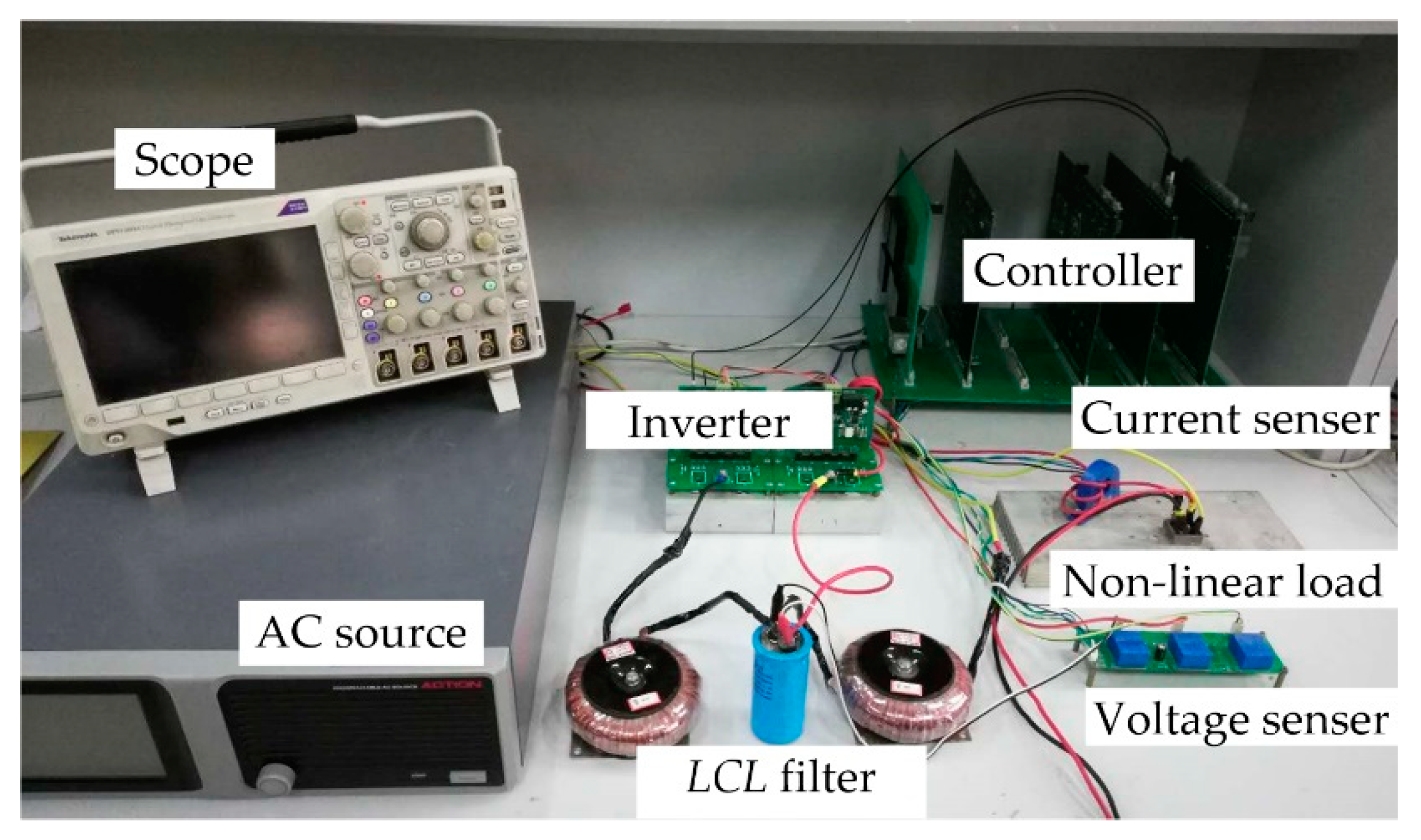
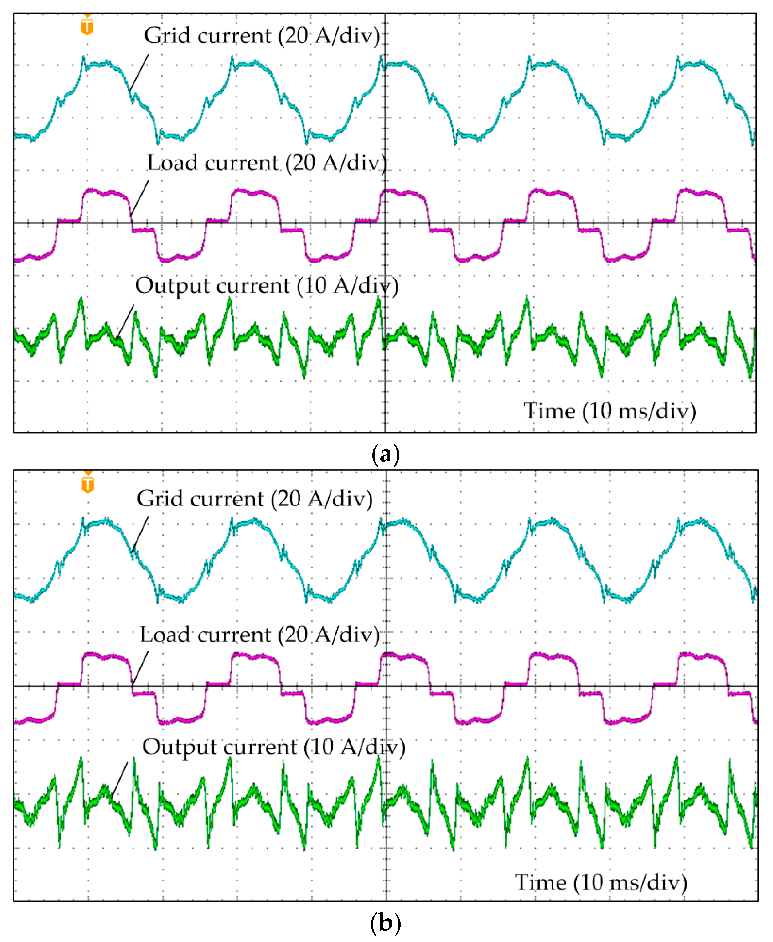
6.2. Experiment
7. Conclusions
Author Contributions
Funding
Conflicts of Interest
References
- Lu, Z.; Li, H.; Qiao, Y. Probabilistic Flexibility Evaluation for Power System Planning Considering Its Association with Renewable Power Curtailment. IEEE Trans. Power Syst. 2018, 33, 3285–3295. [Google Scholar] [CrossRef]
- Nejabatkhah, F.; Li, Y.W. Overview of Power Management Strategies of Hybrid AC/DC Microgrid. IEEE Trans. Power Electron. 2015, 30, 7072–7089. [Google Scholar] [CrossRef]
- Oureilidis, K.O.; Demoulias, C.S. An enhanced role for an energy storage system in a microgrid with converter-interfaced sources. J. Eng. 2014, 11, 618–625. [Google Scholar] [CrossRef]
- Hossain, M.A.; Pota, H.R.; Issa, W.; Hossain, M.J. Overview of AC Microgrid Controls with Inverter-Interfaced Generations. Energies 2017, 10, 1300. [Google Scholar] [CrossRef]
- Kallamadi, M.; Sarkar, V. Generalised analytical framework for the stability studies of an AC microgrid. J. Eng. 2016, 6, 171–179. [Google Scholar] [CrossRef] [Green Version]
- Li, Y.; Wu, M.; Li, Z. A Real Options Analysis for Renewable Energy Investment Decisions under China Carbon Trading Market. Energies 2018, 11, 1817. [Google Scholar] [CrossRef]
- Agrawal, R.; Jain, S. Multilevel inverter for interfacing renewable energy sources with low/medium- and high-voltage grids. IET Renew. Power Gener. 2017, 11, 1822–1831. [Google Scholar] [CrossRef]
- Han, Y.; Li, H.; Shen, P.; Coelho, E.A.; Guerrero, J.M. Review of Active and Reactive Power Sharing Strategies in Hierarchical Controlled Microgrids. IEEE Trans. Power Electron. 2017, 32, 2427–2451. [Google Scholar] [CrossRef]
- Chilipi, R.R.; Al Sayari, N.; Beig, A.R.; Al Hosani, K. A Multitasking Control Algorithm for Grid-Connected Inverters in Distributed Generation Applications Using Adaptive Noise Cancellation Filters. IEEE Trans. Energy Convers. 2016, 31, 714–727. [Google Scholar] [CrossRef]
- He, J.; Li, Y.W.; Blaabjerg, F.; Wang, X. Active Harmonic Filtering Using Current-Controlled, Grid-Connected DG Units With Closed-Loop Power Control. IEEE Trans. Power Electron. 2014, 29, 642–653. [Google Scholar] [CrossRef] [Green Version]
- He, J.; Li, Y.W.; Munir, M.S. A Flexible Harmonic Control Approach through Voltage-Controlled DG–Grid Interfacing Converters. IEEE Trans. Ind. Electron. 2012, 59, 444–455. [Google Scholar] [CrossRef]
- Liu, Y.; Lai, C.-M. LCL Filter Design with EMI Noise Consideration for Grid-Connected Inverter. Energies 2018, 11, 1646. [Google Scholar] [CrossRef]
- Xu, J.; Xie, S.; Huang, L.; Ji, L. Design of LCL-filter considering the control impact for grid-connected inverter with one current feedback only. IET Power Electron. 2017, 10, 1324–1332. [Google Scholar] [CrossRef]
- Hren, A.; Mihalič, F. An Improved SPWM-Based Control with Over-Modulation Strategy of the Third Harmonic Elimination for a Single-Phase Inverter. Energies 2018, 11, 881. [Google Scholar] [CrossRef]
- He, J.; Li, Y.W. Hybrid voltage and current control approach for DG grid interfacing converters with LCL filters. IEEE Trans. Ind. Electron. 2013, 60, 1797–1809. [Google Scholar] [CrossRef]
- Jalili, K.; Bernet, S. Design of LCL filters of active-front-end two level voltage-source converters. IEEE Trans. Ind. Electron. 2009, 56, 1674–1689. [Google Scholar] [CrossRef]
- Tang, Y.; Yao, W.; Loh, P.C.; Blaabjerg, F. Design of LCL Filters with LCL Resonance Frequencies beyond the Nyquist Frequency for Grid-Connected Converters. IEEE J. Emerg. Sel. Top. Power Electron. 2016, 4, 3–14. [Google Scholar] [CrossRef]
- Tang, Y.; Loh, P.C.; Wang, P.; Choo, F.H.; Gao, F.; Blaabjerg, F. Generalized design of high performance shunt active power filter with output LCL filter. IEEE Trans. Ind. Electron. 2012, 59, 1443–1452. [Google Scholar] [CrossRef]
- Said-Romdhane, M.B.; Naouar, M.W.; Belkhodja, I.S.; Monmasson, E. An Improved LCL Filter Design in Order to Ensure Stability without Damping and Despite Large Grid Impedance Variations. Energies 2017, 10, 336. [Google Scholar] [CrossRef]
- Wu, T.F.; Misra, M.; Lin, L.C.; Hsu, C.W. An Improved Resonant Frequency Based Systematic LCL Filter Design Method for Grid-Connected Inverter. IEEE Trans. Ind. Electron. 2017, 64, 6412–6421. [Google Scholar] [CrossRef]
- Wu, W.; Liu, Y.; He, Y.; Chung, H.S.; Liserre, M.; Blaabjerg, F. Damping Methods for Resonances Caused by LCL-Filter-Based Current-Controlled Grid-Tied Power Inverters: An Overview. IEEE Trans. Ind. Electron. 2017, 64, 7402–7413. [Google Scholar] [CrossRef]
- Tang, Y.; Loh, P.C.; Wang, P.; Choo, F.H.; Gao, F. Exploring Inherent Damping Characteristic of LCL-Filters for Three-Phase Grid-Connected Voltage Source Inverters. IEEE Trans. Power Electron. 2012, 27, 1433–1443. [Google Scholar] [CrossRef]
- Liu, F.; Zhou, Y.; Duan, S.; Yin, J.; Liu, B.; Liu, F. Parameter design of a two-current-loop controller used in a grid-connected inverter system with LCL filter. IEEE Trans. Ind. Electron. 2009, 56, 4483–4491. [Google Scholar] [CrossRef]
- Lorzadeh, I.; Askarian Abyaneh, H.; Savaghebi, M.; Bakhshai, A.; Guerrero, J.M. Capacitor Current Feedback-Based Active Resonance Damping Strategies for Digitally-Controlled Inductive-Capacitive-Inductive-Filtered Grid-Connected Inverters. Energies 2016, 9, 642. [Google Scholar] [CrossRef] [Green Version]
- Jin, W.; Li, Y.; Sun, G.; Bu, L. H∞ Repetitive Control Based on Active Damping with Reduced Computation Delay for LCL-Type Grid-Connected Inverters. Energies 2017, 10, 586. [Google Scholar] [CrossRef]
- Yao, W.; Yang, Y.; Zhang, X.; Blaabjerg, F.; Loh, P.C. Design and Analysis of Robust Active Damping for LCL Filters Using Digital Notch Filters. IEEE Trans. Power Electron. 2017, 32, 2360–2375. [Google Scholar] [CrossRef]
- Chen, C.; Xiong, J.; Wan, Z.; Lei, J.; Zhang, K. A Time Delay Compensation Method Based on Area Equivalence for Active Damping of an LCL-Type Converter. IEEE Trans. Power Electron. 2017, 32, 762–772. [Google Scholar] [CrossRef]
- Pan, D.; Ruan, X.; Wang, X. Direct Realization of Digital Differentiators in Discrete Domain for Active Damping of LCL-Type Grid-Connected Inverter. IEEE Trans. Power Electron. 2018, 33, 8461–8473. [Google Scholar] [CrossRef]
- Zhou, S.; Zou, X.; Zhu, D.; Tong, L.; Kang, Y. Improved Capacitor Voltage Feedforward for Three-Phase LCL-Type Grid-Connected Converter to Suppress Start-Up Inrush Current. Energies 2017, 10, 713. [Google Scholar] [CrossRef]
- He, J.; Li, Y.W.; Bosnjak, D.; Harris, B. Investigation and Active Damping of Multiple Resonances in a Parallel-Inverter-Based Microgrid. IEEE Trans. Power Electron. 2013, 28, 234–246. [Google Scholar] [CrossRef]
- Nie, C.; Wang, Y.; Lei, W.; Chen, M.; Zhang, Y. An Enhanced Control Strategy for Multiparalleled Grid-Connected Single-Phase Converters with Load Harmonic Current Compensation Capability. IEEE Trans. Ind. Electron. 2018, 65, 5623–5633. [Google Scholar] [CrossRef]
- Liu, J.; Miura, Y.; Ise, T. Comparison of Dynamic Characteristics between Virtual Synchronous Generator and Droop Control in Inverter-Based Distributed Generators. IEEE Trans. Power Electron. 2015, 31, 3600–3611. [Google Scholar] [CrossRef]
- Xu, H.; Zhang, X.; Liu, F.; Shi, R.; Yu, C.; Cao, R. A Reactive Power Sharing Strategy of VSG Based on Virtual Capacitor Algorithm. IEEE Trans. Ind. Electron. 2017, 64, 7520–7531. [Google Scholar] [CrossRef]
- Liu, Z.; Liu, J.; Zhao, Y. A Unified Control Strategy for Three-Phase Inverter in Distributed Generation. IEEE Trans. Power Electron. 2014, 29, 1176–1191. [Google Scholar] [CrossRef]


| Symbol | Value | Symbol | Value |
|---|---|---|---|
| L1 | 0.6 mH | Vdc | 600 V |
| L2 | 0.6 mH | Vgrid | 380 V (50 Hz) |
| Cf | 6 μF | Kp | 30 |
| Lgrid | 0.1 mH | fs | 20 kHz |
| Harmonic Order | 5th | 7th | 11th | 13th | 17th | 19th | 23th | 25th | 29th |
|---|---|---|---|---|---|---|---|---|---|
| θ | 7.6° | 10.7° | 16.8° | 19.9° | 26.2° | 29.4° | 35.7° | 38.9° | 45.6° |
| α (%) | 1.2 | 2.5 | 6.0 | 8.4 | 14.5 | 18.2 | 26.6 | 31.4 | 42.5 |
| Control Mode | α/% | ||||||||
|---|---|---|---|---|---|---|---|---|---|
| 5th | 7th | 11th | 13th | 17th | 19th | 23th | 25th | 29th | |
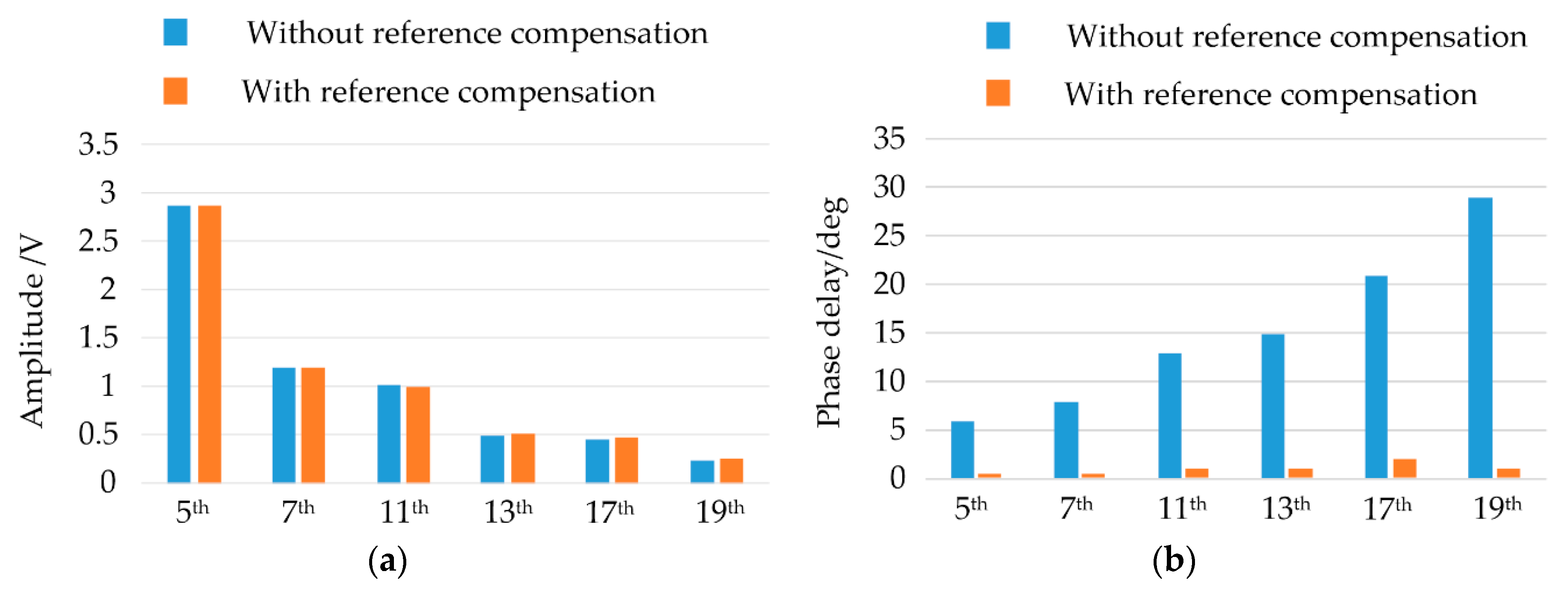
| Without reference compensation | 1.2 | 2.5 | 6.0 | 8.4 | 14.5 | 18.2 | 26.6 | 31.4 | 42.5 |
| With reference compensation | 0.1 | 0.2 | 0.4 | 0.6 | 1.3 | 1.5 | 2.6 | 3.5 | 5.6 |
| Symbol | L1 = L2 | Cf | fr | fLPF |
|---|---|---|---|---|
| 1 | 0.8 mH | 4.5 μF | 3700 Hz | 2653 Hz |
| 2 | 0.6 mH | 6 μF | ||
| 3 | 0.4 mH | 9 μF | ||
| 4 | 0.2 mH | 18 μF |
© 2018 by the authors. Licensee MDPI, Basel, Switzerland. This article is an open access article distributed under the terms and conditions of the Creative Commons Attribution (CC BY) license (http://creativecommons.org/licenses/by/4.0/).
Share and Cite
Nie, C.; Wang, Y.; Lei, W.; Li, T.; Yin, S. Modeling and Enhanced Error-Free Current Control Strategy for Inverter with Virtual Resistor Damping. Energies 2018, 11, 2499. https://doi.org/10.3390/en11102499
Nie C, Wang Y, Lei W, Li T, Yin S. Modeling and Enhanced Error-Free Current Control Strategy for Inverter with Virtual Resistor Damping. Energies. 2018; 11(10):2499. https://doi.org/10.3390/en11102499
Chicago/Turabian StyleNie, Cheng, Yue Wang, Wanjun Lei, Tian Li, and Shiyuan Yin. 2018. "Modeling and Enhanced Error-Free Current Control Strategy for Inverter with Virtual Resistor Damping" Energies 11, no. 10: 2499. https://doi.org/10.3390/en11102499