1. Introduction
Nowadays, permanent magnetic synchronous motors (PMSMs) have been widely applied in electric vehicle, train, electric aircraft, and so on, due to high efficiency and high torque/ampere ratio [
1,
2]. Many control algorithms for PMSMs have been widely researched and successfully applied to a wide range of drive applications [
3].
The proportional integral (PI) controller is a traditional control algorithm that has been widely applied in industry. Since the control system of PMSMs is a nonlinear system with unavoidable disturbances and parameter variations, it is difficult for the PI controller to obtain a satisfying dynamic performance in the entire operating range [
4]. A lot of intelligence control algorithms are also proposed, such as sliding mode control [
5,
6], adaptive control [
7,
8], neural network control [
9,
10], and so on. However, their dependence on the motor parameters and heavy computation load limit their application on PMSMs.
Recently, model-based predictive control (MPC) strategies have received attention in research communities due to their faster dynamic response, precise steady-state performance, easy implementation, and easy inclusion of nonlinearities and constraints [
11,
12,
13]. MPC can be classified into two types: the finite set MPC (FSMPC) and the continuous-time MPC (CTMPC) [
14].
FSMPC exploits the inherent discrete nature of power converters, does not require a modulator, has an intuitive concept, and is easy to understand. Among all available FSMPC in power electronics, predictive current control (PCC) and predictive torque control (PTC) are two most popular control methods [
15].
There are main challenges of the PCC in industrial deployment, such as the uncertainty of model parameters [
16,
17], measurement noise [
18], and varying switching frequency [
19]. Ref. [
20] analyzed the parameter sensitivity of PCC and adopted a disturbance observer (SCDO) to track the disturbance caused by parameter mismatch. PCC with Kalman filtering and inductance profile auto-calibration was presented in [
21], which aimed to improve the performance of switched reluctance motors (SRMs) current control. To achieve a constant switching frequency and improve transient characteristics under faster speed changing, the proposed controller in [
22] combined deadbeat control and PCC techniques. However, the complexity of the controller was increased. PTC was proposed recently as an effective control scheme in the application of high performance torque control of motor drives. The vector selection of PTC is more effective than conventional direct torque control (DTC), which uses a switching table [
23,
24]. The cost function of PTC usually consists of torque and flux magnitude errors, which are different in unit and magnitude, where a proper weighting factor is required to achieve satisfactory performance [
25]. To reduce the torque ripple of PTC, an improved PTC applied in an inductance motor (IM) was proposed based on the inherent relationship between the stator current and stator flux [
26]. A simplified PTC was presented in [
27] based on a new switching table, where both the number of prediction vectors and the computational load were reduced by considering the position of stator flux and the sign of torque deviation.
CTMPC is one of the most popular formulations among the MPC algorithms, and has been successfully implemented in industry [
28]. CTMPC only considers the past and present tracking errors and can ensure the near-optimal performance of the system by minimizing a cost function. Moreover, CTMPC requires a pulse-width modulation (PWM) modulator, but it is designed to deal, especially, with non-linear systems having fast dynamics [
29]. A novel CTMPC approach was proposed in [
30] for the control of sensorless induction motors (IMs). The multivariable CTMPC controller allowed the rotor flux and speed tracking simultaneously while considering constraints of voltage and current. In [
31], a nonlinear CTMPC for IMs had been developed. It included system state variables of stator currents, as well as rotor flux and speed. The rotor speed, flux and the load torque were estimated using an extended Kalman filter (EKF). A CTMPC of PMSMs with disturbance decoupling was proposed in [
32]. The predicted speed tracking error was directly used to determine the required voltage command without the need of a cascaded control scheme. Ref. [
33] presented a robust continuous nonlinear model predictive control (CNMPC) for a grid-connected photovoltaic (PV) inverter system. The objective of the proposed approach was to control the power exchange between the grid and the PV system, while achieving unity power factor operation.
This paper proposed an improved CTMPC of PMSMs for a wide-speed range including the constant torque region and flux-weakening (FW) region. In the constant torque region, a linear mathematic model of PMSMs is presented to predict dq-axes voltages. In the FW region, since dq-axes voltages are coupled together due to the limitation of DC-link voltage, a nonlinear mathematic model of CTMPC of PMSMs based on the voltage angle control is proposed. Since solving the complicated mathematical model of PMSMs in the FW region will cost a lot of time, the increment of voltage angle is linearized at each sample instant to predict the system future dynamics and reduce computation load for digital signal processing (DSP). The smooth transitions between the constant torque region and the FW region are also considered and presented in this paper.
This paper is organized as follows: The principle of CTMPC is analyzed in
Section 2. In
Section 3, the proposed improved CTMPC is shown; this section is divided into three parts: CTMPC in the constant torque region, CTMPC in the FW region, and the smooth transition between them. The simulation and experiment results are presented in
Section 4. This paper is concluded with a summary in
Section 5.
2. Continuous-Time Model Predictive Control
The predictive algorithm of CTMPC involves a class of control techniques, which utilize a process model to predict the system future behavior, with the control law obtained by optimizing a cost function that considers the following: (1) the effort necessary for control, and (2) the difference between predicted output values and reference values. In order to apply the first element of the optimal sequence, a receding-horizon principle is adopted. Since the future behavior of the system needs to be predicted, the model of the system is the core of CTMPC. A discrete-time state-space model is considered as the follows:
where
x(
k)
is the state variable,
u(
k)
is the input variable,
yc(
k)
is the output variable, and
d(
k)
is the disturbance from outside which can be measured.
A,
Bu,
Bd, and
Cc are the coefficients of variables respectively.
To reduce the steady-state error of the output, the prediction is derived by Equations (3) and (4) with an incremental model.
where
;
;
.
The predicted output of system is given by (5)
where
yc(
k + 1|
k) is the predicted output at instant
k + 1 based on the output at instant
k.
To make sure the predicted output is close to the reference output, the following cost function is adopted.
where
Γy and
Γu are weight coefficients.
Γy is a defined positive variable, allowing an emphasis on each of the controlled outputs and its predictions.
Γu is a defined positive variable, which weights the control efforts of inputs.
rj (
k + 1) is the reference output variable.
A new variable is defined as follows in order to obtain the minimum value of cost function.
where
Then, the cost function can be rewritten as follows:
The minimum value of cost function can be calculated by:
Since the second derivation of (8) is bigger than zero (Equation (10)), the extreme value of cost function is the minimum value.
The minimum value of cost function is:
The optimal incremental input at instant
k is
where Δ
u*(
k) is the optimal incremental input at instant
k.
Constraints are inevitable in system, such as the extreme values, increment of control variables, and so on. Usually, these constraints are presented as follows:
where
ymin(
k) and
ymax(
k) are the minimum and maximum values of output variable, respectively,
umin(
k) and
umax(
k) are the minimum and maximum values of input variable, respectively, and Δ
umin(
k) and Δ
umax(
k) are the minimum and maximum incremental values of input variable, respectively.
3. Improved CTMPC of PMSMs for a Wide-Speed Range
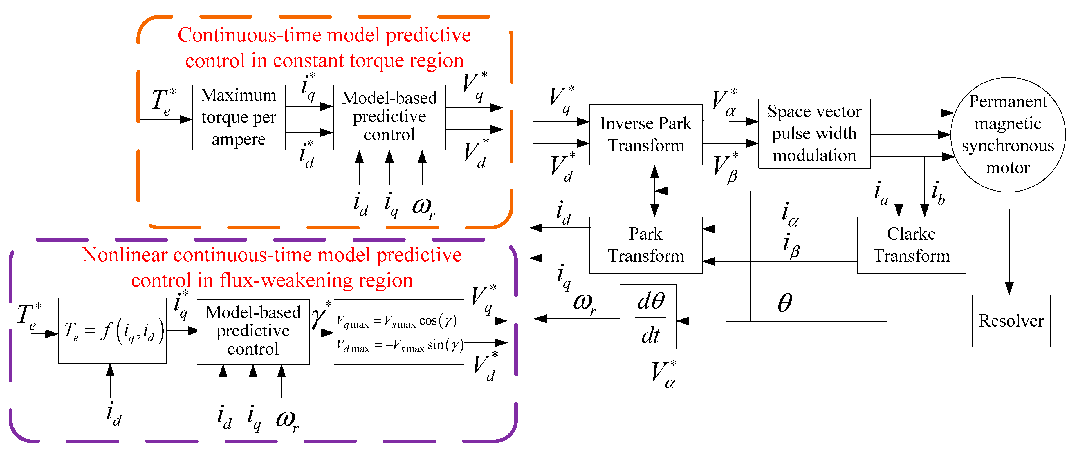
Improved CTMPC control algorithms of PMSMs are proposed in this paper. The block diagram of the proposed control system is shown in
Figure 1. The proposed algorithms can be applied for a wide-speed range including the constant torque region and the FW region. In the constant torque region, one CTMPC control algorithm is proposed based on the maximum torque per ampere (MTPA) control to increase system efficiency. In the FW region, another CTMPC is proposed according to the nonlinear property of PMSMs driven system. The detailed introduction of the control diagram will be elaborated in the following text.
3.1. CTMPC of PMSMs in the Constant Torque Region
The mathematical model of PMSMs drive system can be described by the following equations in synchronous rotating dq reference frame:
where
Rs: Stator winding resistance;
id, iq: d and q axes currents;
vd, vq: d and q axes voltages;
Ld, Lq: d and q axes inductances;
ωr: Electrical speed in rad/sec;
λf: Magnet flux linkage;
vs: The output voltage of inverter;
vsmax: The maximum output voltage of inverter limited by the DC-link voltage.
In the constant torque region, the output voltag e (vs) of the inverter is smaller than the maximum output voltage of the inverter (vsmax). Without the DC-link voltage limitations, the PMSMs mathematical model is a linear equation group. The relationship of dq-axes voltages (vd, vq) can be decoupled. Due to the decoupling relationship of vd and vq, the solutions of id and iq will be many groups when the reference torque and speed are given. The id and iq, which can minimize the system currents, will be adopted to increase system efficiency called MTPA control.
In DSP, the continuous-time representation of system model has to be transformed into a discrete-time representation based on the forward Euler approximation with a sampling period
Ts.
where
Ts is a constant sampling time substituting for
dt.
With the transformations of (16), the discrete-time PMSMs model can be obtained as follows
where
.
In the discrete-time PMSMs model, id(k) and iq(k) are considered as the state variables and the output variables simultaneously. vd(k) and vq(k) are considered as the input variables. ωr(k) is considered to be an external disturbance which can be measured.
To reduce the steady-state error of the dq-axes currents, an incremental model of PMSMs is applied as follows.
Equation (21) is the cost function of CTMPC which means that the actual dq-axes currents are changing close to the reference values.
where
iq(
k + 1|
k) and
id(
k + 1|
k) are the predicted dq-axes currents at instant
k + 1 based on dq-axes currents at instant
k;
i*q(
k + 1) and
i*d(
k + 1) are the reference dq-axes currents at instant
k + 1.
By the minimization of the cost function (21), the optimal increment of input voltages at instant
k can be obtained by (22) based on (12) in numerical method.
where Δ
v*q(
k) and Δ
v*d(
k) are the optimal incremental dq-axs voltages at instant
k.
To limit the extreme values and the increment of the input voltages, the following constraints are applied in the CTMPC.
where Δ
vqmax and Δ
vdmax are the maximum incremental values of dq-axes voltages.
3.2. CTMPC of PMSMs Based on Voltage Angle Control in the Flux-Weakening Region
In the FW region, the maximum output voltage (
vsmax) of the inverter is limited by DC-link voltage (
VDC). According to the location of
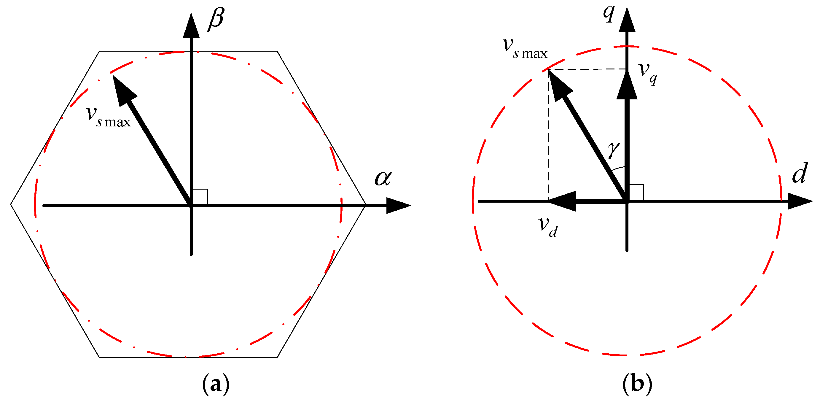
vsmax in the hexagon of the stationary αβ frame,
vsmax varies from
to 2
VDC/3 shown in
Figure 2a. In this paper,
vsmax is set to
to increase the DC-link voltage utilization level and reduce torque ripple.
Figure 2b shows the vector diagram of PMSMs in the synchronously rotating frame in the FW region, and
γ is the angle between
vsmax and
vq which is called the voltage angle. Since
vsmax is set to a constant value,
vd and
vq can be represented by:
Consequently, the key of FW control is how to obtain
γ with the restrain of
vsmax. The PMSMs model in the FW region can be rewritten as:
In the FW region, vd and vq are cross-coupled together by the limitation of the DC-link output voltage shown in (24). The mathematical model of PMSMs is changing to a single-input and multiple-output (SIMO) system in the FW region. When dq reference currents (i*d and i*q) are given, γ can be calculated according to (25) since vsmax has been set to a constant value. Therefore, there is only one pair solution of vd and vq. The solution of vd and vq can be obtained by adjusting γ through q-axis voltage equation.
The q-axis discrete-time PMSMs model in the FW region can be rewritten as:
where
,
,
, and
P is the number of poles.
In the q-axis PMSMs model of (26), iq is considered as the state variable and the output variable at the same time, id is one of coefficient in BdFW, while γ is considered as the input variables, and ωr is considered to be the external disturbance which can be measured.
To solve such a complicated nonlinear equation group on line may cause heaven computation load for DSP. Therefore, the increment of voltage angle Δγ is linearized at each sample instant in this paper.
The increment of
vq at instant
k can be calculated based on trigonometric function as:
Assuming Δ
γ(
k) =
γ(
k) −
γ(
k − 1), because the sampling time
Ts is very small that:
where Δ
γ(
k) is the increment of voltage angle at instant
k.
The increment of
vq can be rewritten as:
So far, the control variable Δ
vq*(
k) can be replaced by Δ
γ*(
k) in (26). The voltage angle control can be applied as follows.
where Δ
γ*(
k) is the reference increment of voltage angle
γ(
k) at instant
k.
The incremental model of PMSMs in the FW region is shown as:
The following constrains of
γ are applied to limit the extreme value and increment.
where Δ
γmax is the maximum increment of voltage angle
γ.
In the FW region, the reference current
iq* of PMSMs can be calculated by the reference torque
Te* and
id shown in (33):
The cost function (34) means
iq is changing close to the reference value.
By the minimization of the cost function (30), the optimal incremental voltage angle of driven system at instant
k can be obtained by (34) based on (12).
3.3. Smooth Transition of CTMPC between the Constant Torque Region and the FW Region
Since different CTMPC methods are adopted in the constant torque region and the FW region, the smooth transitions are also studied in this paper.
The smooth transition between the constant torque and the FW regions is primarily to ensure that the actual value of torque is basically the same as the reference value. Two questions about the transition are proposed in this paper. The first one is how to find the point where the constant torque region must switch to the FW region, and the second one is how to find the point where the FW region should change back to the constant torque region.
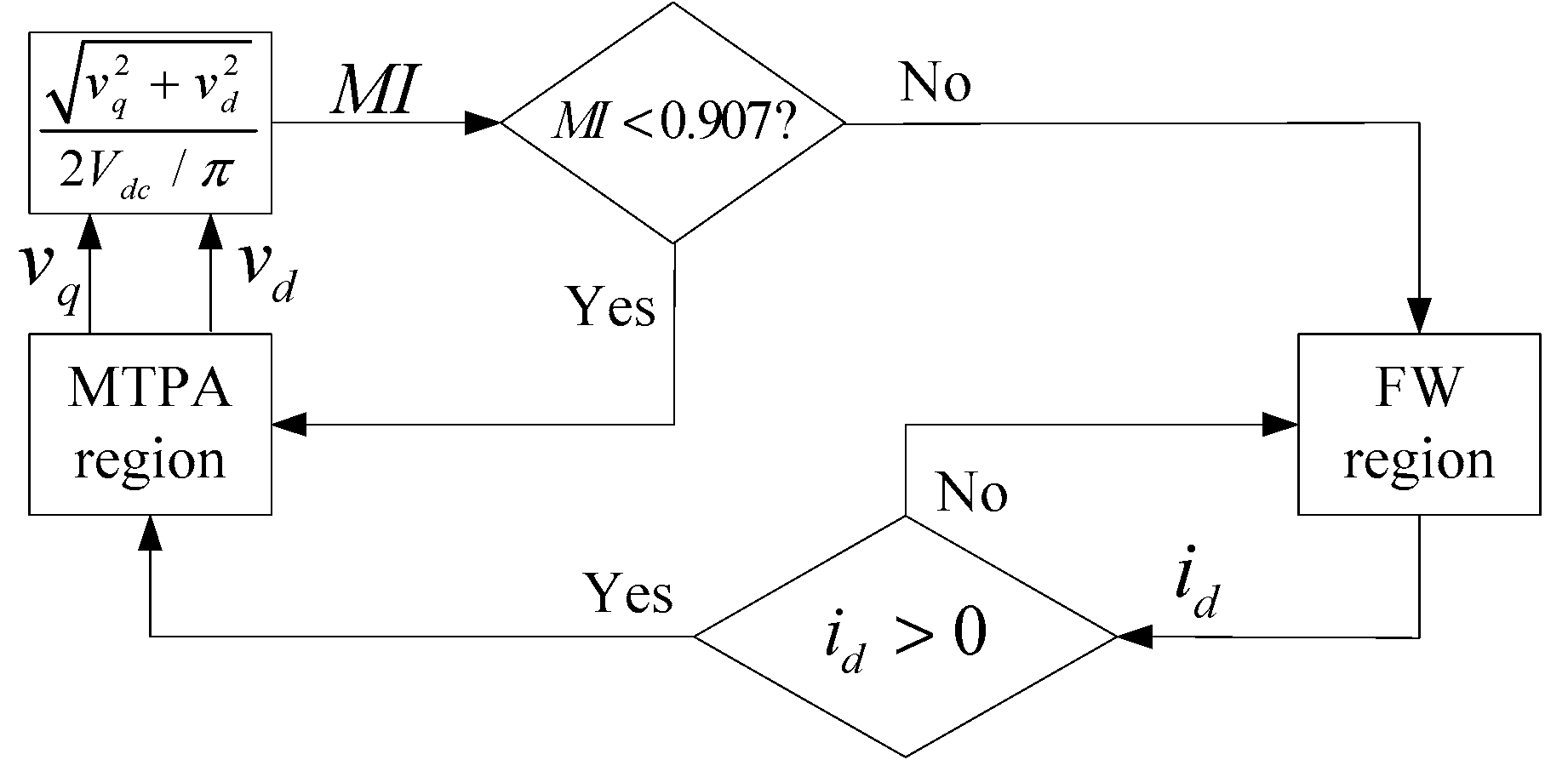
Figure 3 shows the transitions between the constant torque and FW regions. When motors are working in the constant torque region, the modulation index (MI) should be calculated. If MI is smaller than 0.907, the motor will remain working in the constant torque region, and when MI is equal or bigger than 0.907, the motor should work in the FW region. When the motor works in the FW region, the d-axis current is used as the switching condition since MI is equal to 0.907 during the FW region.
3.3.1. The Constant Torque Region Transiting to the FW Region
At the point where the constant torque region should change to the FW region, according to (15), iq, id, and ωr are three important state variables in the transiting point selection. Besides these, the DC-link voltage, MI, parameters of driven system (such as resistance, inductance), and the nonlinearity of the inverter can also influence the selection of transiting point. Consequently, the selection of transiting point under changing parameters is difficult.
In this paper, the maximum value of MI is set to 0.907 to balance the utilization level of DC-link voltage and the torque ripple minimization. Therefore, when the MI reaches 0.907 the constant torque region must change to the FW region. MI can be calculated by (36).
After the transiting point is determined, the initial value of
γ0 has to be calculated. If
γ0 is chosen improperly, the output torque will deviate from the reference value. Consequently, the initial value of
γ0 is another important problem to ensure the smooth transition. The relationship between d-q axes voltage and
γ0 is (37), since both of the constant torque control and the FW control algorithms are applicable at the transiting point.
where
vd0,
vq0 are d-q axes voltages at the transiting point.
The initial value of voltage angle
γ0 can be calculated by:
3.3.2. The FW Region Changes Back to the Constant Torque Region
Due to the decreasing of reference speed/torque or the rising of DC-link voltage, FW region should change back to the constant torque region. Since MI is a control parameter, it is impossible to determine the transiting point based on MI. Now, we will analyze the influence on dq-axes currents if adopting FW control algorithm on the constant torque region under the same reference torque and speed.
In the constant torque region with the same reference torque and speed, if the FW control algorithm is adopted, the value of
vs will be
vsmax which is bigger than required. Under this circumstance, the currents under the FW control algorithm will be bigger than the constant torque control algorithm according to (15), shown as follows.
where
iq_MTPA and
id_MTPA are dq-axis currents in constant torque region when the MTPA control algorithm is adopted,
iq_FW and
id_FW are dq-axis currents in constant torque region when the FW control algorithm is adopted.
For surface mounted PMSMs (SMPMSM), the q-axis current will not change under the same output torque regardless what control algorithm is adopted since the d-axis current cannot produce torque. Therefore the higher part of currents will be d-axis current. Consequently, the transiting point where the FW region should return back to the constant torque region is when
id is bigger than zero. For interior PMSMs (IPMSMs), the d-axis current can produce reluctance torque because
Lq is bigger than
Ld. However, the q-axis current has the main contribution to output torque contrasting with reluctance torque. The higher part of current will also be d-axis current when FW control algorithm is adopt in the constant torque region. The transiting point where the FW region should return back to the constant torque region is as follows:
Simulations have been performed with an 110 kW IPMSM. Parameters of the IPMSM are shown in
Table 1.
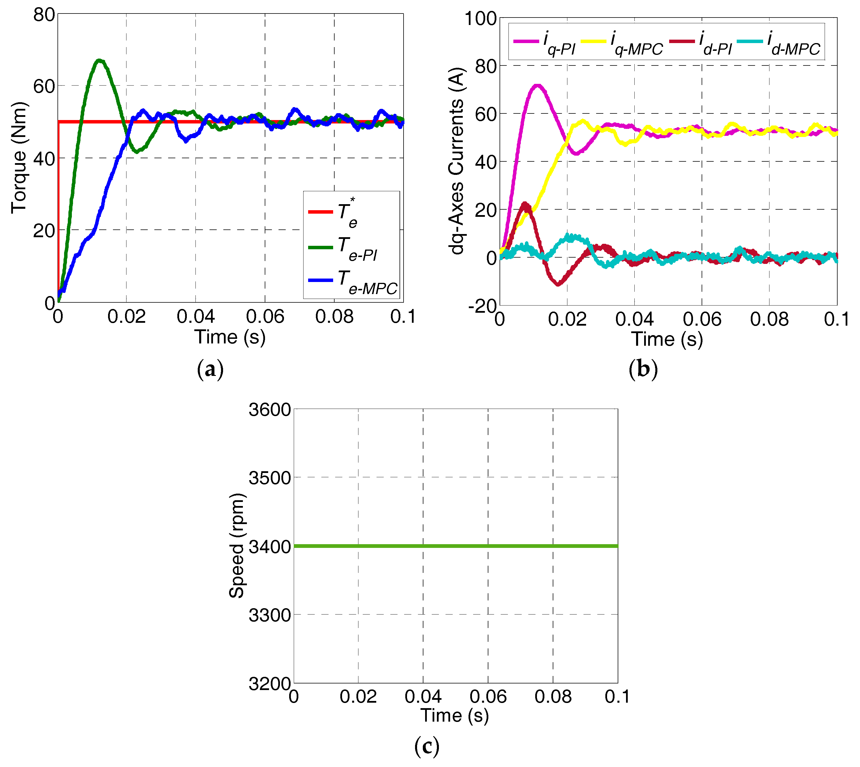
Figure 4 shows the simulation results under step torque changing of CTMPC and PI controller. Both of the output torque of CTMPC and PI controller can track the reference torque very well shown in
Figure 4a. The response speed of CTMPC and PI controller is about 0.02 s. Under PI controller, in order to enhance the response speed, the overshoot currents are inevitable shown in
Figure 4b, while CTMPC can achieve the same response speed without any overshoot. For a high-power IPMSMs-driven system, in order to increase the power density of the inverter and reduce the cost, the margin of the inverter is limited. With the increase of the working current, the overshoot current under step torque changing may exceed the maximum current which the inverter can bear, and result in the damage of the inverter. Therefore, if the CTMPC proposed in this paper is adopted, the security of driven system will be increased.
Besides, for a high-power IPMSMs-driven system, in order to protect the inverter, the maximum values of dv/dt and di/dt should be limited. With those limitations, the response speeds of CTMPC and PI are slower than standard controllers.
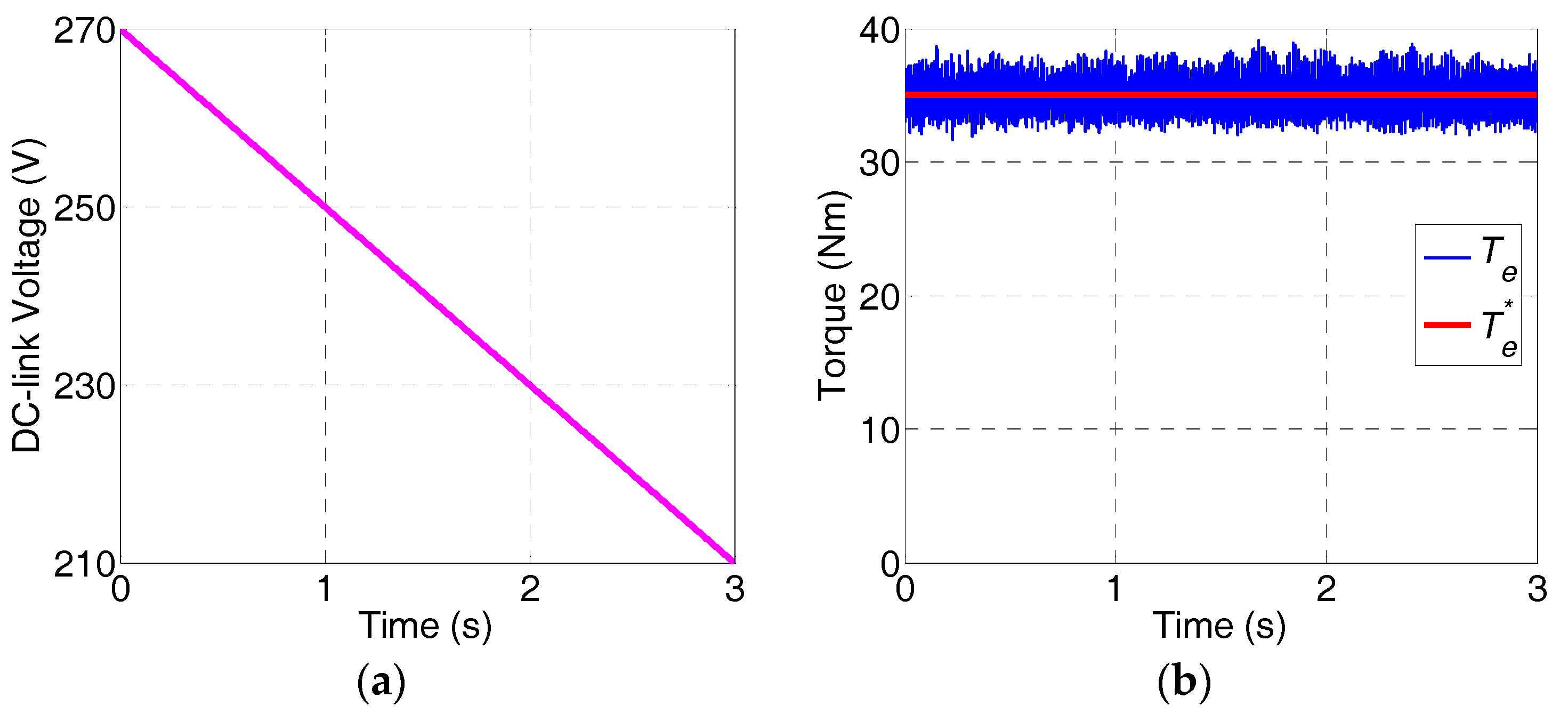
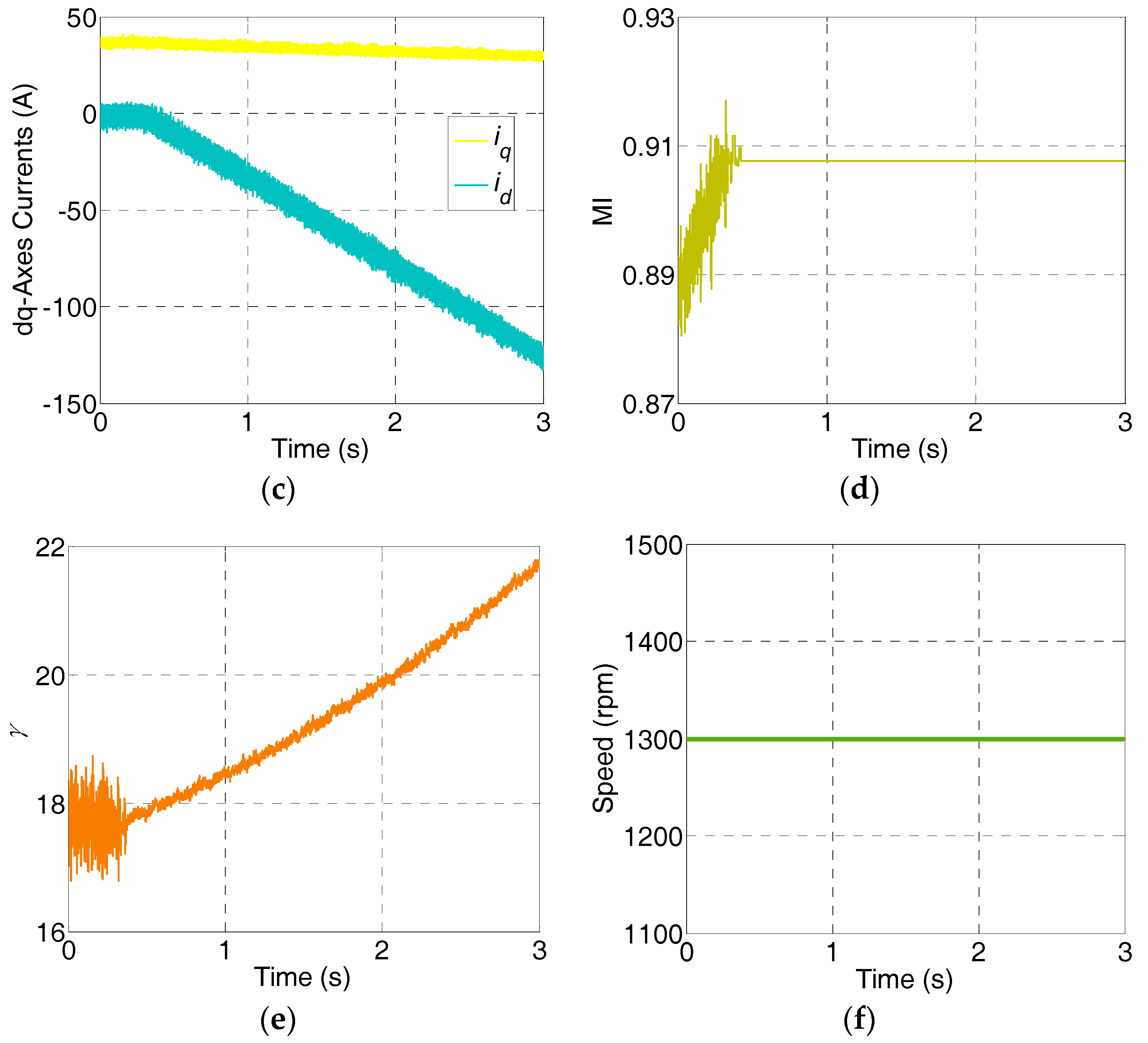
Figure 5 is the simulation results under an adjustable DC-link voltage ranging from 270 V to 210 V at 1300 rpm. The reference torque is 35 Nm during simulation. With the decreasing of DC-link voltage, MI is increased as shown in
Figure 5d. After 0.4 s, since the MI is equal or bigger than 0.907, the working condition of the motor changes to the FW region from the constant torque region. Then, the demagnetizing current (
id) is increased significantly with the decreasing of the DC-link voltage shown in
Figure 5c. Simultaneously,
γ changes from 17.5° to 21.5° (
Figure 5e). It should be noted that during simulation,
iq maintains on 36.6 A basically. The simulation results indicate that the proposed CTMPC can ensure the smooth transition between the constant torque region and the FW region under the adjustable DC-link voltage since the output torque can track the reference value very well, as shown in
Figure 5b. The simulation results also indicate that the area of FW region is enlarged, owing to the decreasing of DC-link voltage. For a given speed and torque, the operation (constant torque or FW) may be different according to DC-link voltage. Therefore, it is important to determine the transiting point by MI.
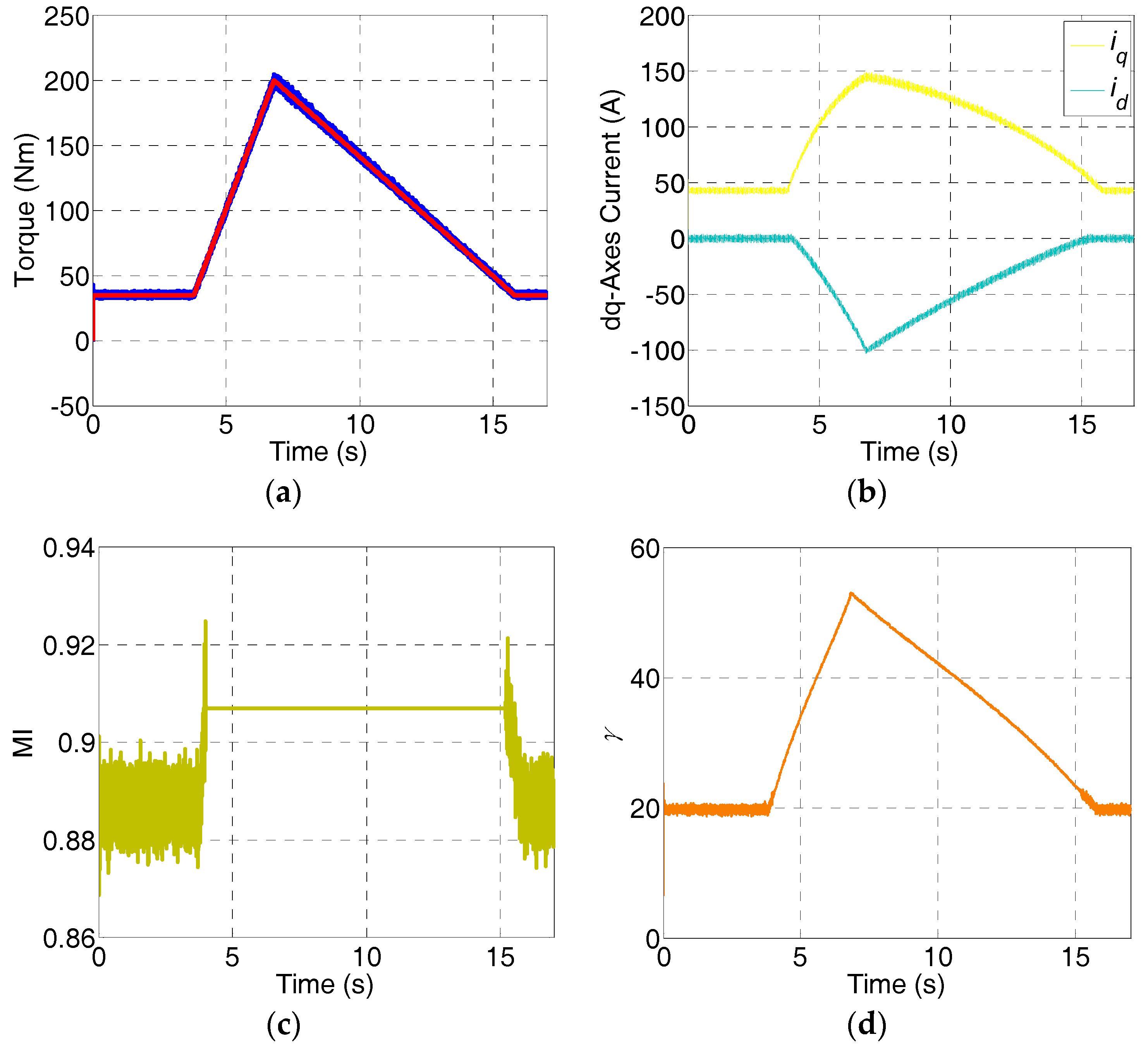
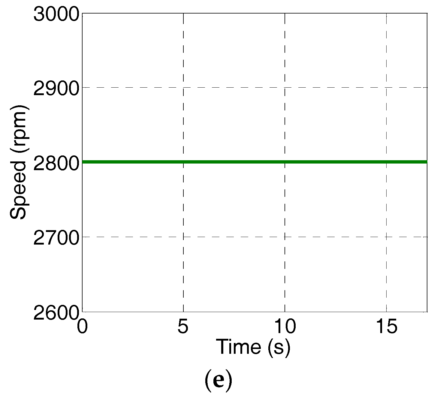
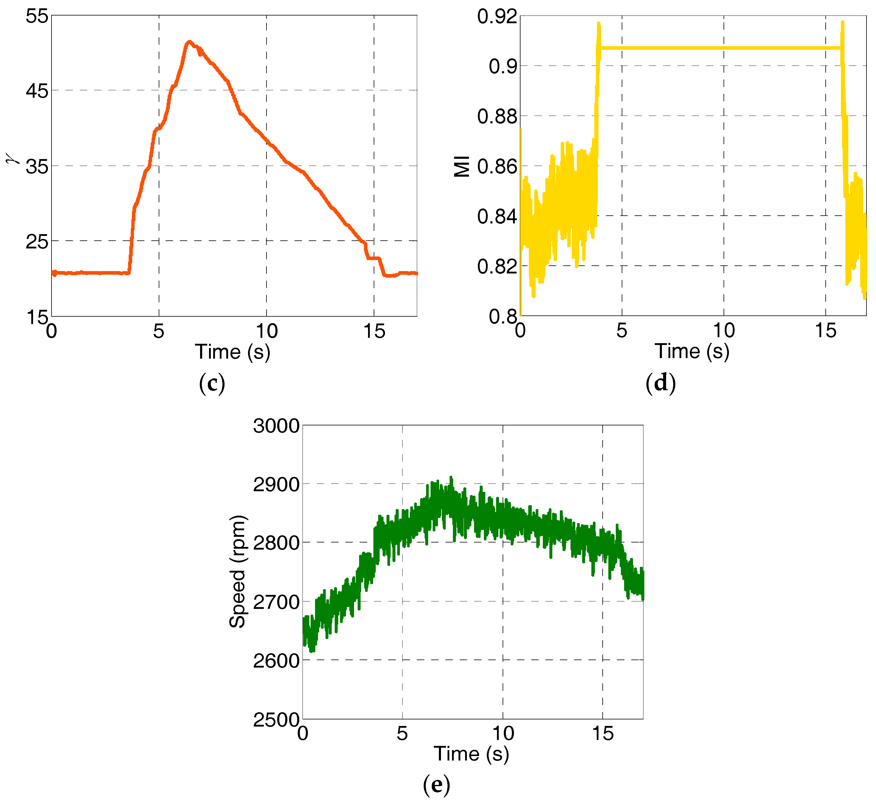
Figure 6 shows the simulation results with the IPMSM entering and leaving the FW region with the changing of reference torque. During 0–4 s, the reference torque is 50 Nm. After that, the reference torque increases slowly to 200 Nm at 7 s. Then, the reference torque decreases to 50 Nm at 16 s. During 16–17 s, the reference torque is 50 Nm again. With the increasing of torque shown in
Figure 6a, MI (
Figure 6c) increases, too. When MI reaches the maximum value 0.907 (about 4 s), the constant torque region changes into the FW region. During 4–7 s,
id and
γ both increase with the increase of the reference torque as shown in
Figure 6b,d. After that,
id and
γ both decrease because of the decrease of the output torque. When
id equals to 0 at about 20 s (
Figure 6b), IPMSM leaves the FW region. With the proposed method, the IPMSM can be controlled very well on the FW region. The proposed method can realize the seamless transition between the two modes.
4. Experiment Results
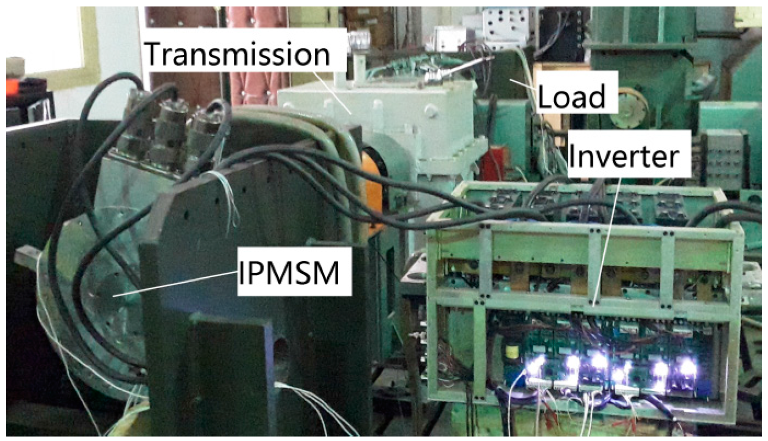
The experimental setup includes an inverter, an IPMSM, a transmission, and a load shown in
Figure 7. The transmission can change the transmission ratio of driven system, and expand its working scope. The load is another IPMSM which works as a generator. It can keep the driven system working at the given speed. A host PC is used to run the user interface (RS-232 connected) and the DSP development and debugger tools (JTAG connected). RS-232 is applied to send instructions to the inverter and receive signals from the inverter. The communication speed of RS-232 is about 0.5 s. The controller area network (CAN) of the DSP is used to collect the signals of control variables and state variables since the communication speed of RS-232 is lower than CAN, such as MI,
γ, DC-link voltage, currents, speed, etc. The communication speed of the CAN is 250 kbps.
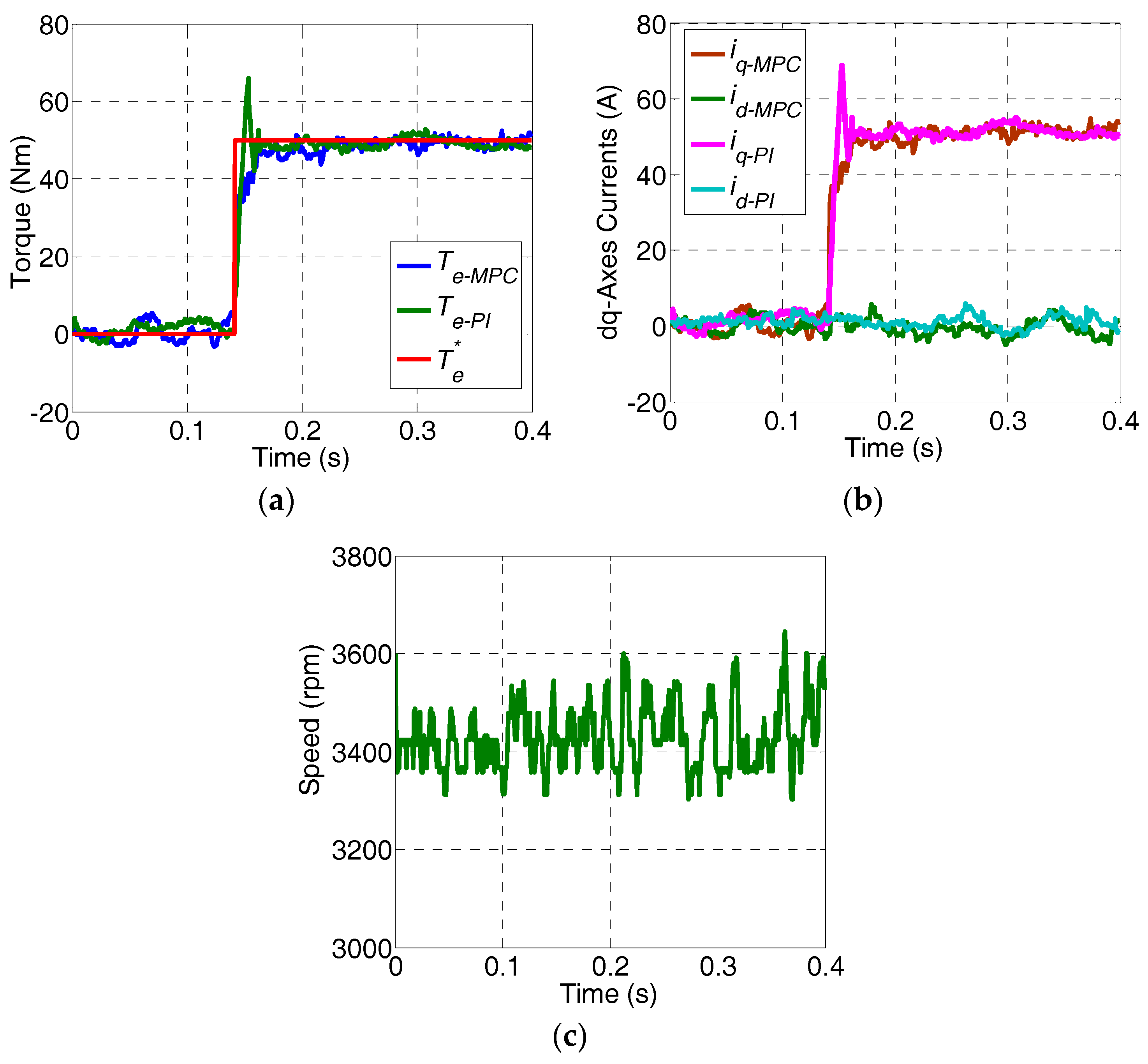
Figure 8 shows the experiment results under the step torque changing of CTMPC and PI controller. The reference torque is 50 Nm. Both the output torque of the CTMPC and PI controller can track the reference value accurately. The response speed of CTMPC and PI controller is about 0.02 s. When CTMPC is adopted, the overshoot phenomenon is restrained which is one of the advantages of CTMPC.
The simulation and experimental results of proposed CTMPC and PI controller with step torque changing are basically the same. However, constrained by the communication speed of CAN, simulation results can reveal more details than experimental results.
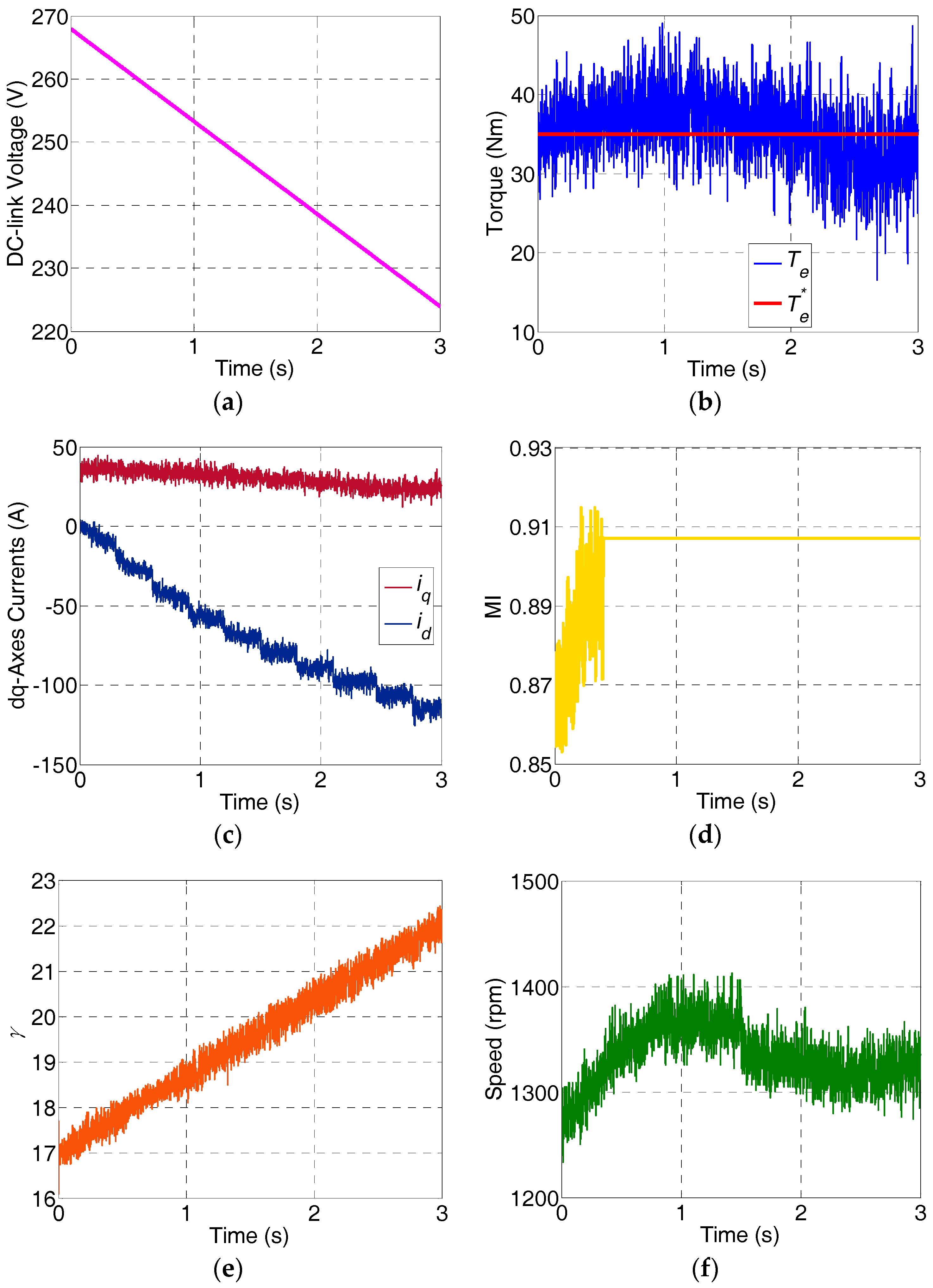
Figure 9 shows the experiment results of proposed CTMPC under the adjustable DC-link voltage. The DC-link voltage is changing from 268 V to 224 V during experiment as shown in
Figure 9a. The reference torque is 35 Nm, and the output torque can track the reference value basically shown in
Figure 9b. With the decreasing of DC-link voltage, at about 0.4 s, MI is increasing to 0.907. The working state of IPMSM is switching to the FW region from the constant torque region. The experimental results show that the proposed CTMPC can ensure the smooth transition between the constant torque region and FW region under changeable DC-link voltage.
During the experiment, the speed of driven system is maintained by the other IPMSM, which works as load. The speed of driven system is 1325 rpm basically shown in
Figure 9f. Compared with simulation results under the adjustable DC-link voltage (
Figure 5), speed fluctuations are more obvious.
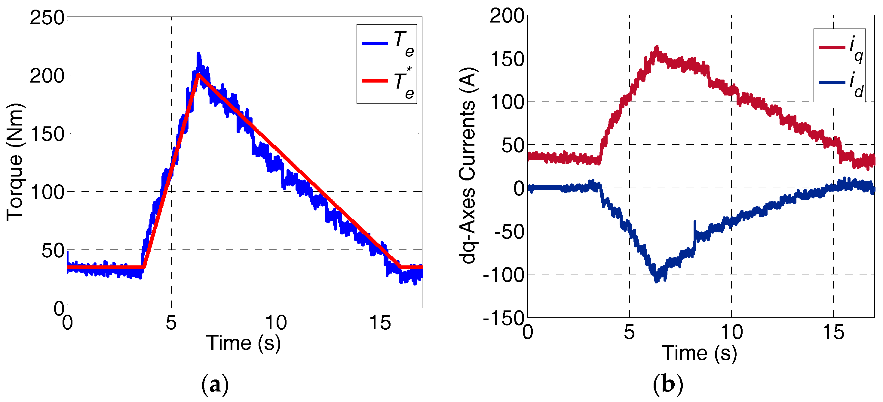
Figure 10 shows the experiment results of the proposed CTMPC during entering and leaving FW region by the changing of the reference torque. During the experiment, the changing of reference torque is the same with simulation. At about 4 s, when MI is reaching to 0.907, the work state of IPMSM is switching to the FW region from the constant region. At about 16 s, when
id is decreasing to 0, the work state of IPMSM is switching back to the constant region from the FW region. During experiment, the output torque can track the references basically according to
Figure 10a. Therefore, the proposed CTMPC can ensure the smooth transition between the constant torque and FW regions under the changing output torque.
5. Conclusions
Two CTMPC models are proposed to describe the properties of PMSMs in the constant torque region and the FW region respectively for the aim of performance improvement. Due to the limitation of the DC-link voltage, the mathematical model of PMSMs in FW region is nonlinear, so the increment of the voltage angle is linearized at each sample time. Therefore, the proposed CTMPC has obvious advantages in dealing with systems non-linear constrains and reducing computation load of DSP. Besides, the proposed CTMPC can restrain the overshoot current with torque step changing, which can enhance the safety of inverter. The selection of transition points between the constant torque region and the FW region is also presented. Both simulation and experimental results show that the proposed CTMPC can ensure the smooth transition between the constant torque and FW regions even under changing DC-link voltage and torque.
Some additional issues will be addressed in the future, including the improving of torque accuracy, the robustness of the controller, and the increasing of the response speed.


