

A Tree Attenuation Factor Model for a Low-Power Wide-Area Network in a Ruby Mango Plantation †

Abstract
:1. Introduction
1.1. Related Work
1.2. Contribution
- TAFs are proposed for a Ruby mango plantation. These factors can be used for both short- and long-distance path loss prediction with an accuracy comparable to conventional regression models.
- An exponential decay model is modified to be suitable for Ruby mango plantations.
- RSSI measurement data were captured for a LoRa LPWAN in the 433 MHz frequency channel.
2. Proposed Path Loss Models
2.1. ABC Model
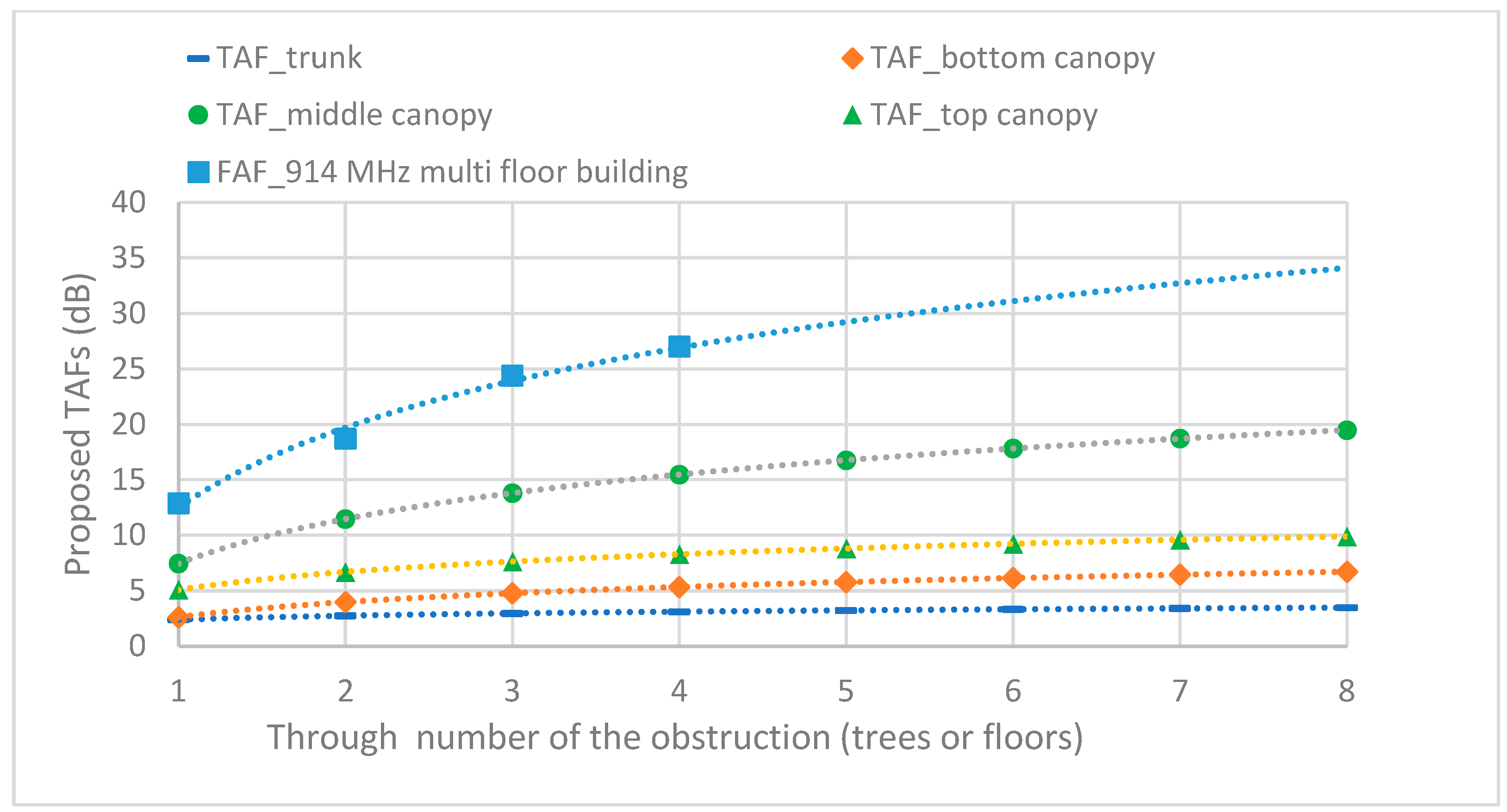
2.2. Tree Attenuation Factors Model
3. Field Measurements
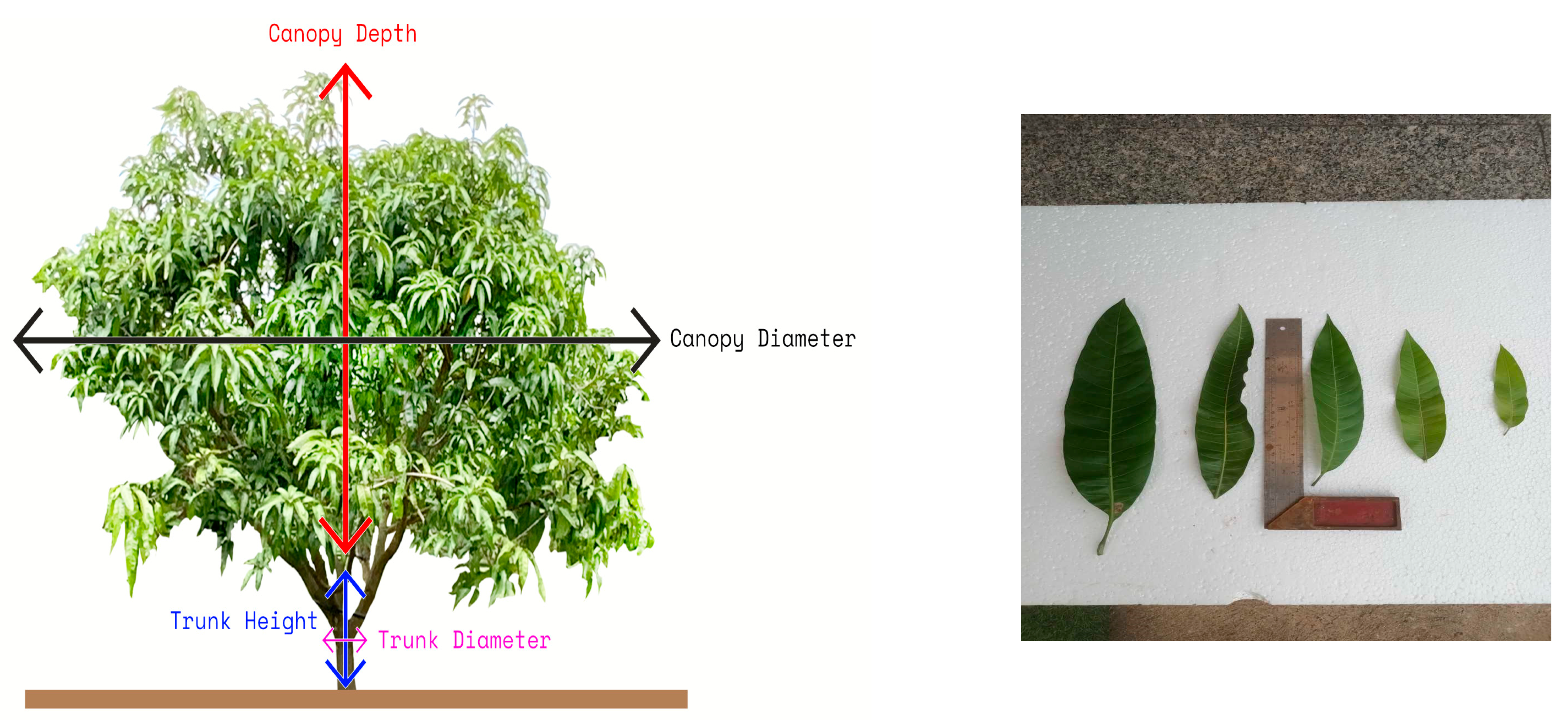
3.1. Site Description
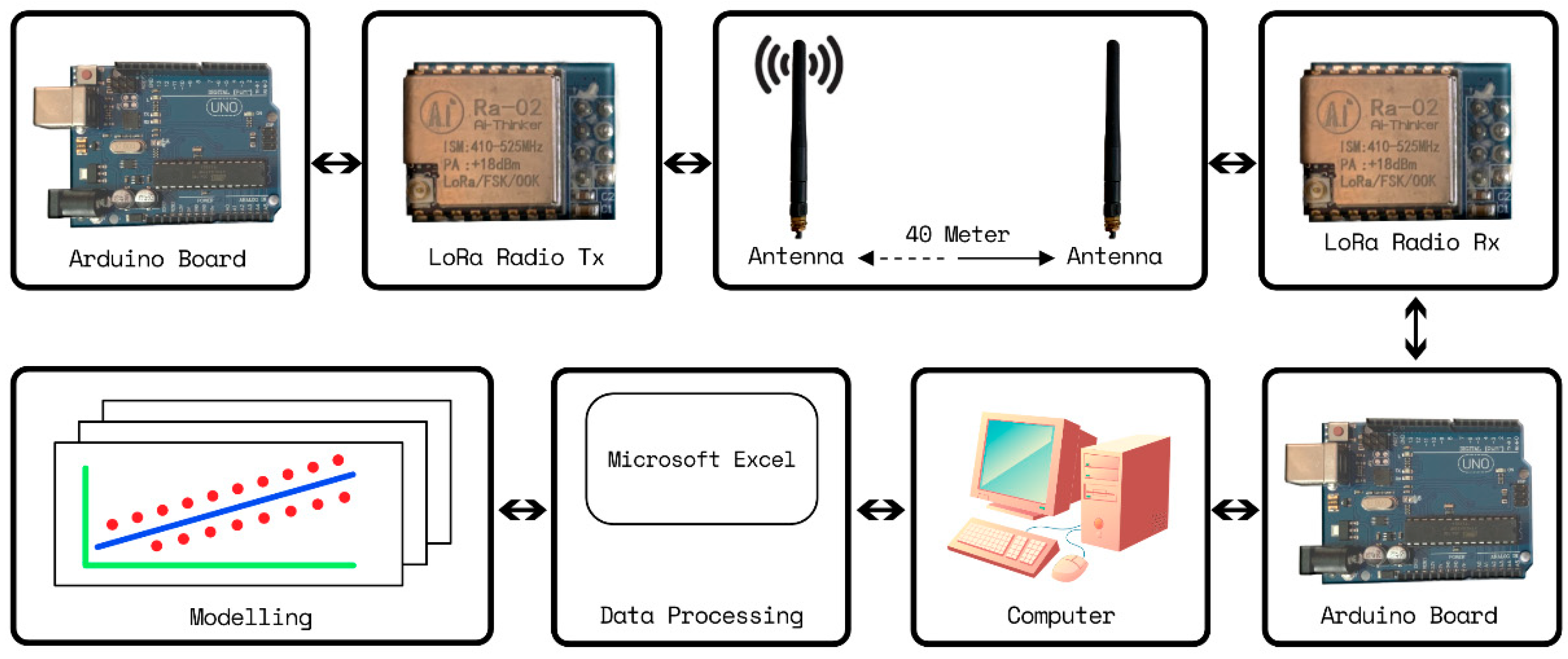
3.2. Measurement Setup
4. Results and Discussion
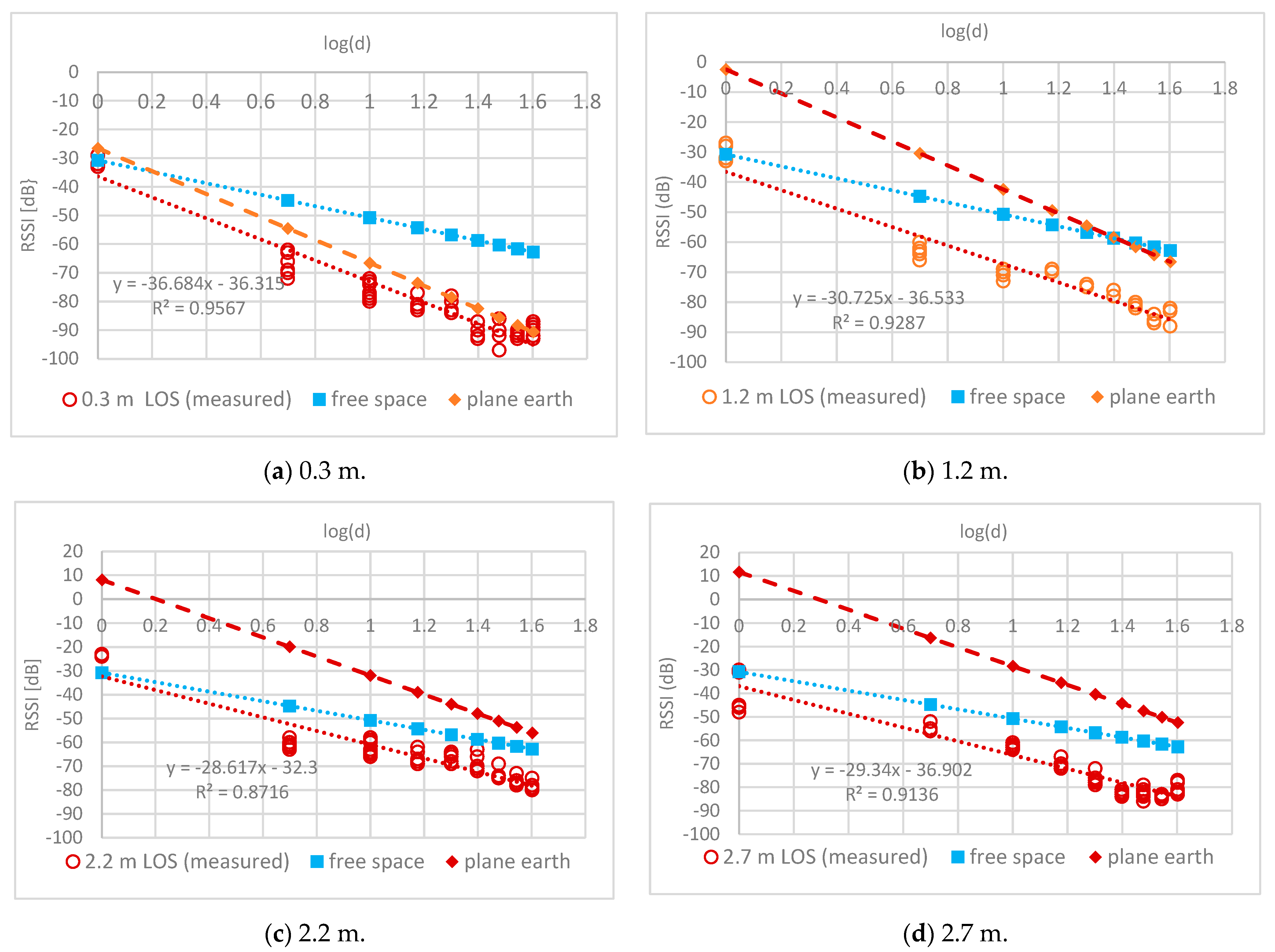
4.1. LOS Routes
- -
- Trunk level (h = 0.3 m)
- -
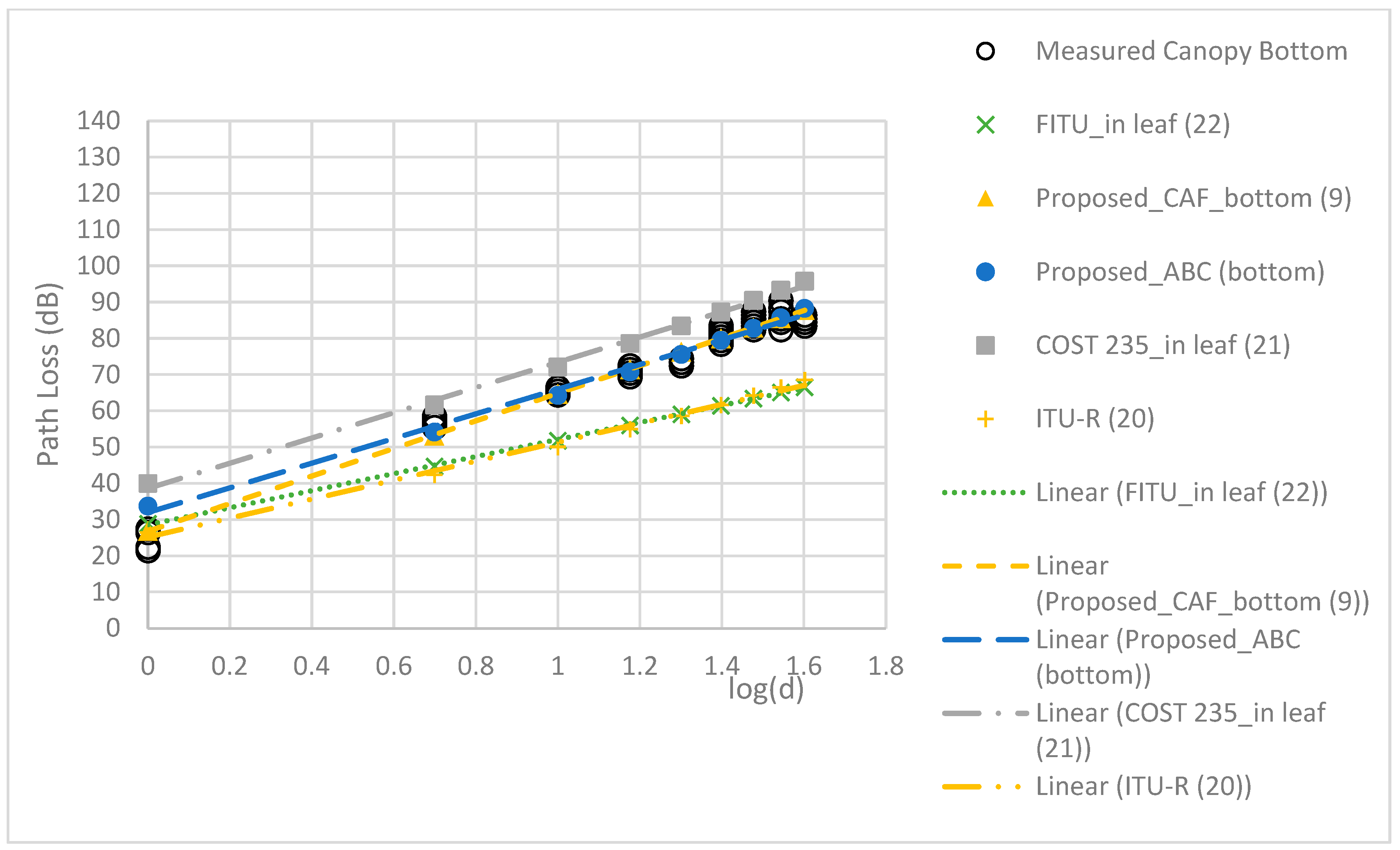
- Bottom canopy level (h = 1.2 m)
- -
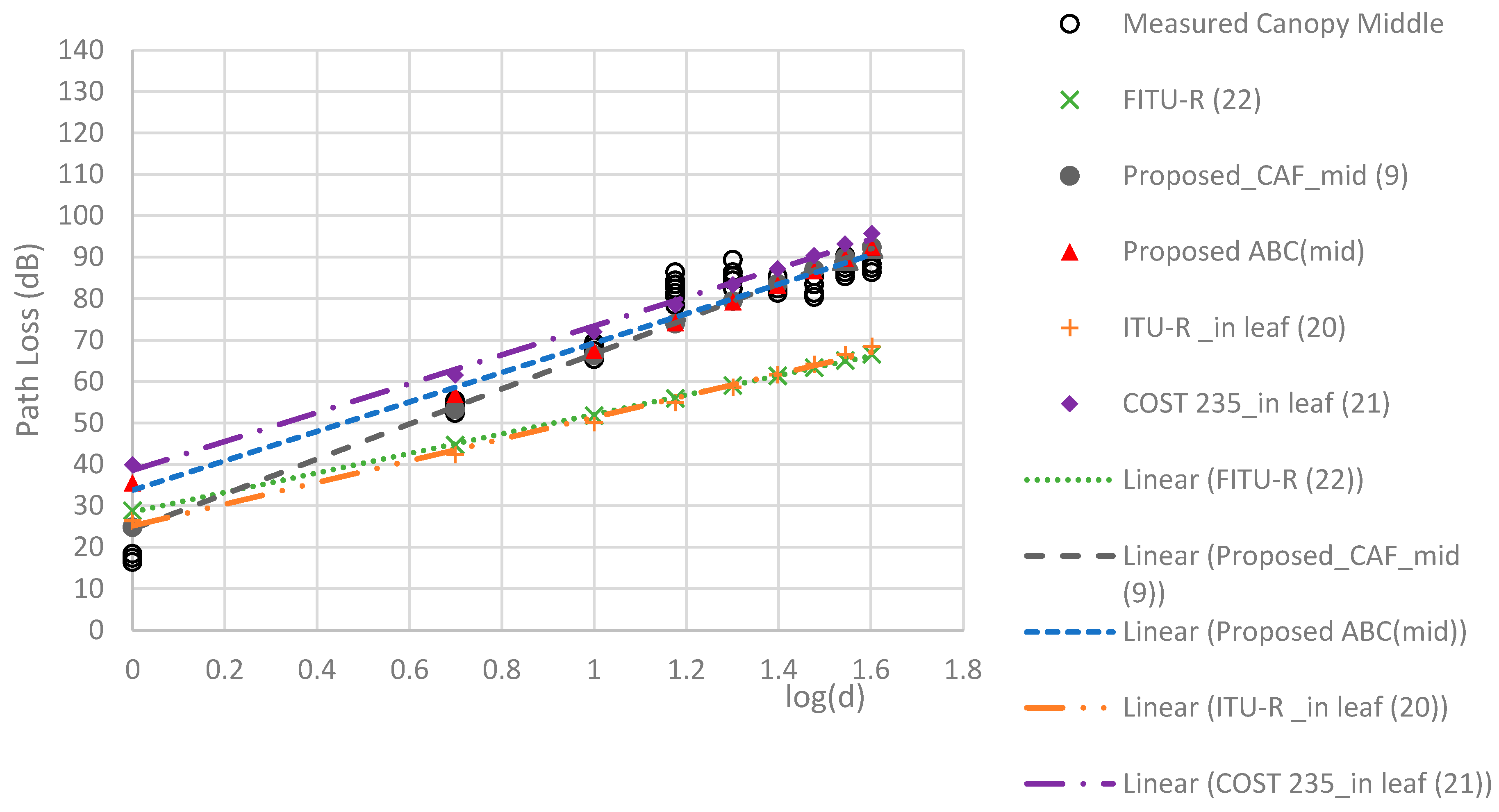
- Middle canopy level (h = 2.2 m)
- -
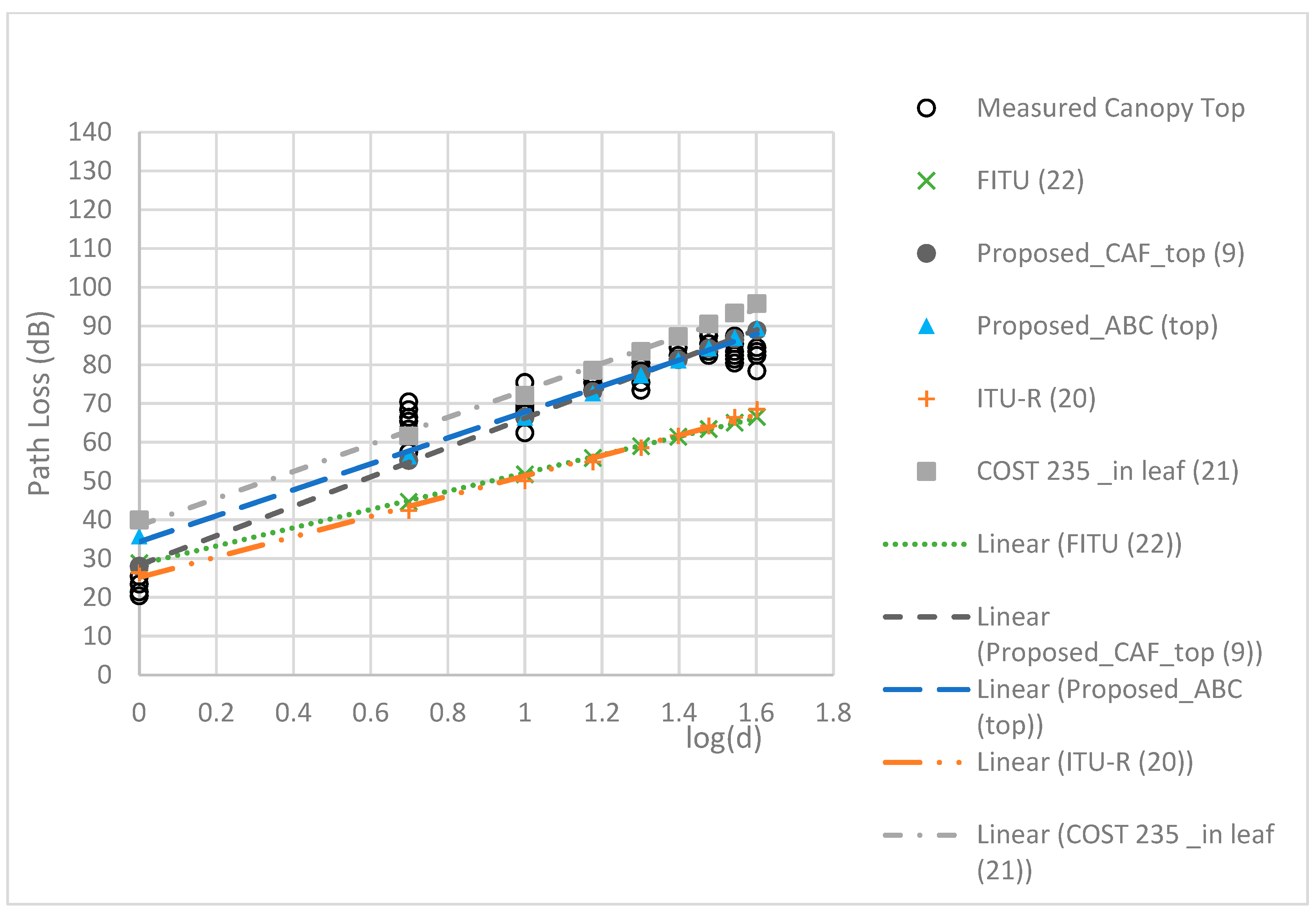
- Top canopy level (h = 2.7 m)
4.2. NLOS Routes
- -
- Trunk level (h = 0.3 m)
- -
- Bottom canopy level (h = 1.2 m)
- -
- Middle canopy level (h = 2.2 m)
- -
- Top canopy level (h = 2.7 m)
4.3. Model Comparison
- (1)
- ITU-R Foliage Attenuation Model
- (2)
- COST 235 Model
- (3)
- FITU-R Foliage Attenuation with Plane-Earth Model
5. Conclusions
Author Contributions
Funding
Institutional Review Board Statement
Informed Consent Statement
Data Availability Statement
Acknowledgments
Conflicts of Interest
References
- Available online: https://www.boi.go.th (accessed on 10 January 2023).
- Shaikh, F.K.; Karim, S.; Zeadally, S.; Nebhen, J. Recent trends in internet-of-things-enabled sensor technologies for smart agriculture. IEEE Internet Things J. 2022, 9, 23583–23598. [Google Scholar] [CrossRef]
- Elijah, O.; Rahman, T.A.; Orikumhi, I.; Leow, C.Y.; Hindia, M.N. An overview of Internet of Things (IoT) and data analytics in agriculture: Benefits and challenges. IEEE Internet Things J. 2018, 5, 3758–3773. [Google Scholar] [CrossRef]
- Jani, K.A.; Chaubey, N.K. A Novel Model for Optimization of Resource Utilization in Smart Agriculture System Using IoT (SMAIoT). IEEE Internet Things J. 2022, 9, 11275–11282. [Google Scholar]
- Pagano, A.; Croce, D.; Tinnirello, I.; Vitale, G. A Survey on LoRa for Smart Agriculture: Current Trends and Future Perspectives. IEEE Internet Things J. 2022, 10, 3664–3679. [Google Scholar] [CrossRef]
- Citoni, B.; Fioranelli, F.; Imran, M.A.; Abbasi, Q.H. Internet of Things and LoRaWAN-Enabled Future Smart Farming. IEEE Internet Things Mag. 2019, 2, 14–19. [Google Scholar]
- Pinto, D.C.; Damas, M.; Holgado-Terriza, J.A.; Arrabal-Campos, F.M.; Gómez-Mula, F.; Martínez-Lao, J.A.M.; Cama-Pinto, A. Empirical Model of Radio Wave Propagation in the Presence of Vegetation inside Greenhouses Using Regularized Regressions. Sensors 2020, 20, 6621. [Google Scholar] [CrossRef]
- Abouzar, P.; Michelson, D.G.; Hamdi, M. RSSI-based distributed self-localization for wireless sensor networks used in precision agriculture. IEEE Trans. Wirel. Commun. 2016, 15, 6638–6650. [Google Scholar]
- Akbas, A.; Yildiz, H.U.; Tavli, B.; Uludag, S. Joint Optimization of Transmission Power Level and Packet Size for WSN Lifetime Maximization. IEEE Sens. J. 2016, 16, 5084–5094. [Google Scholar] [CrossRef]
- Meng, Y.S.; Lee, Y.H. Investigations of foliage effect on modern wireless communication systems: A review. Prog. Electromagn. Res. 2010, 105, 313–332. [Google Scholar] [CrossRef]
- Leite, D.L.; Alsina, P.J.; Campos, M.M.; Sousa, V.A.; Medeiros, A.M. Unmanned Aerial Vehicle Propagation Channel over Vegetation and Lake Areas: First- and Second-Order Statistical Analysis. Sensors 2022, 22, 18. [Google Scholar] [CrossRef]
- Raheemah, A.; Sabri, N.; Salim, M.S.; Ehkan, P.; Ahmad, R.B. New empirical path loss model for wireless sensor networks in mango greenhouses. Comput. Electron. Agric. 2016, 127, 553–560. [Google Scholar]
- Anzum, R.; Habaebi, M.H.; Islam, R.; Hakim, G.P.N.; Khandaker, M.U.; Osman, H.; Alamri, S.; Elrahim, E.A. A multiwall path-loss prediction model using 433 MHz LoRa-WAN frequency to characterize foliage’s influence in a Malaysian palm oil plantation environment. Sensors 2022, 22, 5397. [Google Scholar] [CrossRef]
- Anderson, C.R.; Volos, H.I.; Buehrer, R.M. Characterization of low-antenna ultrawideband propagation in a forest environment. IEEE Trans. Veh. Technol. 2013, 62, 2878–2895. [Google Scholar] [CrossRef]
- Azevedo, J.; Santos, F.E.S. An empirical propagation model for forest environments at tree trnk level. IEEE Trans. Antennas Propag. 2011, 59, 2357–2367. [Google Scholar] [CrossRef]
- Azevedo, J.; Santos, F.E.S. A model to estimate the path loss in areas with foliage of trees. Int. J. Electron. Commun. 2017, 71, 157–161. [Google Scholar]
- Barrios-Ulloa, A.; Ariza-Colpas, P.P.; Sánchez-Moreno, H.; Quintero-Linero, A.P.; De la Hoz-Franco, E. Modeling radio wave propagation for wireless sensor networks in vegetated environments: A systematic literature review. Sensors 2022, 22, 5285. [Google Scholar] [CrossRef]
- Meng, Y.S.; Lee, Y.H.; Ng, B.C. Empirical near ground path loss modeling in a forest at VHF and UHF bands. IEEE Trans. Antennas Propag. 2009, 57, 1461–1468. [Google Scholar] [CrossRef]
- Tang, W.; Ma, X.; Wei, J.; Wang, Z. Measurement and analysis of near-ground propagation models under different terrains for wireless sensor networks. Sensors 2019, 19, 1901. [Google Scholar] [CrossRef]
- De Jong, Y.L.C.; Herben, M.H.A.J. A tree-scattering model for improved propagation prediction in urban microcells. IEEE Trans. Veh. Technol. 2004, 53, 503–513. [Google Scholar] [CrossRef]
- Leonor, N.; Caldeirinha, R.; Fernandes, T.; Ferreira, D.; Sánchez, M.G. A 2D ray-tracing based model for micro-and millimeter-wave propagation through vegetation. IEEE Trans. Antennas Propag. 2014, 62, 6443–6453. [Google Scholar] [CrossRef]
- Leonor, N.; Sánchez, R.M.G.; Fernandes, T.; Ferreira, D. A 2D ray-tracing based model for wave propagation through forests at micro and millimeter wave frequencis. IEEE Access 2018, 6, 32097–32108. [Google Scholar] [CrossRef]
- Hakim, G.P.N.; Habaebi, M.H.; Toha, S.F.; Islam, M.R.; Yusoff, S.H.B.; Adesta, E.Y.T.; Anzum, R. Near Ground Pathloss Propagation Model Using Adaptive Neuro Fuzzy Inference System for Wireless Sensor Network Communication in Forest, Jungle and Open Dirt Road Environments. Sensors 2022, 22, 3267. [Google Scholar] [CrossRef] [PubMed]
- Wu, L.; He, D.; Ai, B.; Wang, J.; Qi, H.; Guan, K.; Zhong, Z. Artificial Neural Network Based Path Loss Prediction for Wireless Communication Network. IEEE Access 2020, 8, 199523–199538. [Google Scholar]
- Pal, P.; Sharma, R.P.; Tripathi, S.; Kumar, C.; Ramesh, D. NSGA-III Based Heterogeneous Transmission Range Selection for Node Deployment in IEEE 802.15.4 Infrastructure for Sugarcane and Rice Crop Monitoring in a Humid Sub-Tropical Region. IEEE Trans. Wireless Commu. 2023, 22, 3643–3656. [Google Scholar] [CrossRef]
- You, L.; Liu, S.; Chang, Y.; Yuen, C. A triple-step asynchronous federated learning mechanism for client activation, interaction optimization, and aggregation enhancement. IEEE Internet Things J. 2022, 9, 24199–24211. [Google Scholar] [CrossRef]
- Pedro, A.V.; Leni, J.M.; Pedro, V.G.C.; Leonardo, G.; Edson, C. Statistics, Coverage, and Improvement of Modelling via ANN of Radio Mobile Signal in Vegetated Channel in the 700-4000 MHz Band. IEEE Lat. Am. Trans. 2023, 21, 1209–1217. [Google Scholar]
- Shaibu, F.E.; Onwuka, E.E.N.; Salawu, N.; Oyewobi, S.S.; Djouani, K.; Abu-Mahfouz, A.M. Performance of Path Loss Models over Mid-Band and High-Band Channels for 5G Communication Networks: A Review. Future Internet 2023, 15, 362. [Google Scholar] [CrossRef]
- Seidel, S.Y.; Rappaport, T.S. 914 MHz path loss prediction models for indoor wireless communications in multifloored buildings. IEEE Trans. Antennas Propag. 1992, 40, 207–217. [Google Scholar] [CrossRef]
- Onykiienko, Y.; Popovych, P.; Yaroshenko, R.; Mitsukova, A.; Beldyagina, A.; Makarenko, Y. Using RSSI data for LoRa network path loss modeling. In Proceedings of the 2022 IEEE 41st International Conference on Electronics and Nanotechnology (ELNANO), Kyiv, Ukraine, 10–14 October 2022; pp. 576–579. [Google Scholar]
- CCIR. Influences of Terrain Irregularities and Vegetation on Troposphere Propagation; CIR Rep.: Geneva, Italy, 1986; pp. 235–236. [Google Scholar]
- European Commission. Radio Propagation Effects on Next-Generation Fixed-Service Terrestrial Telecommunication Systems; European Commission: Luxembourg, 1996. [Google Scholar]
- Al-Nuaimi, M.O.; Stephens, R.B.L. Measurements and prediction model optimization for signal attenuation in vegetation media at centimetre wave frequencies. Proc. Inst. Elect. Eng. Microw. Antennas Propag. 1998, 145, 201–206. [Google Scholar] [CrossRef]


| No. | Total Height | Trunk Height | Trunk Diameter | Canopy Depth | Canopy Diameter |
|---|---|---|---|---|---|
| Tree 1 | 3.82 | 0.56 | 0.40 | 3.4 | 5.5 |
| Tree 2 | 4.66 | 0.66 | 0.56 | 4.0 | 6.0 |
| Tree 3 | 4.79 | 0.49 | 0.45 | 4.3 | 5.6 |
| Tree 4 | 5.15 | 0.65 | 0.64 | 4.5 | 6.5 |
| Tree 5 | 4.77 | 0.47 | 0.63 | 4.3 | 6.2 |
| Tree 6 | 3.96 | 0.46 | 0.46 | 3.5 | 4.7 |
| Tree 7 | 4.85 | 0.65 | 0.54 | 4.2 | 6.0 |
| Tree 8 | 3.97 | 0.47 | 0.43 | 3.5 | 5.0 |
| Average | 4.50 | 0.55 | 0.51 | 3.96 | 5.69 |
| No. | Parameters | Value | Unit |
|---|---|---|---|
| 1 | Power Amplifier (PA) | 18 | dBm |
| 2 | Antenna gain | 2.2 | dBi |
| 3 | Frequency | 433 | MHz |
| 4 | Bandwidth (BW) | 125 | kHz |
| 5 | Spreading factor | 7 | - |
| 6 | Code rate (CR) | 4/5 | - |
| 7 | Antenna height | 0.3–2.7 | m |
| Antenna Height (m) | PLE (LOS) | PLE (NLOS) | Tree Attenuation Factors | A | B | C | Validation (RMSE) | |
|---|---|---|---|---|---|---|---|---|
| Through | TAF (dB) | |||||||
| 0.3 (trunk) | 3.67 | 3.79 | 1 | 2.40 | 0.98 | 0.39 | 0.34 | 2.11 |
| 2 | 2.76 | |||||||
| 3 | 2.97 | |||||||
| 4 | 3.12 | |||||||
| 5 | 3.24 | |||||||
| 6 | 3.34 | |||||||
| 7 | 3.42 | |||||||
| 8 | 3.49 | |||||||
| 1.2 (bottom canopy) | 3.07 | 3.84 | 1 | 2.62 | 0.8 | 0.39 | 0.35 | 0.42 |
| 2 | 3.98 | |||||||
| 3 | 4.79 | |||||||
| 4 | 5.35 | |||||||
| 5 | 5.79 | |||||||
| 6 | 6.15 | |||||||
| 7 | 6.46 | |||||||
| 8 | 6.72 | |||||||
| 2.2 (middle canopy) | 2.86 | 4.33 | 1 | 7.46 | 0.98 | 0.39 | 0.33 | 0.31 |
| 2 | 11.47 | |||||||
| 3 | 13.81 | |||||||
| 4 | 15.47 | |||||||
| 5 | 16.76 | |||||||
| 6 | 17.82 | |||||||
| 7 | 18.71 | |||||||
| 8 | 19.48 | |||||||
| 2.7 (top canopy) | 2.93 | 3.71 | 1 | 5.09 | 1.0 | 0.39 | 0.3 | 1.18 |
| 2 | 6.70 | |||||||
| 3 | 7.63 | |||||||
| 4 | 8.30 | |||||||
| 5 | 8.82 | |||||||
| 6 | 9.24 | |||||||
| 7 | 9.60 | |||||||
| 8 | 9.91 | |||||||
| Antenna Height (m) | MAE (dB) | ||||
|---|---|---|---|---|---|
| Proposed | ITU-R | COST235 | FITU-R | ||
| TAF | ABC | ||||
| 0.3 (trunk) | 4.79 | 5.54 | 19.63 | 10.19 | 20.55 |
| 1.2 (bottom canopy) | 2.22 | 2.66 | 16.39 | 7.91 | 16.49 |
| 2.2 (middle canopy) | 4.21 | 5.14 | 19.08 | 6.86 | 19.09 |
| 2.7 (top canopy) | 4.13 | 4.96 | 17.69 | 7.45 | 17.84 |
| Average | 3.84 | 4.58 | 18.2 | 8.1 | 18.49 |
| Antenna Height (m) | RMSE (dB) | ||||
|---|---|---|---|---|---|
| Proposed | ITU-R | COST235 | FITU-R | ||
| TAF | ABC | ||||
| 0.3 (trunk) | 6.2 | 7.08 | 21.65 | 11.77 | 22.59 |
| 1.2 (bottom canopy) | 2.65 | 3.69 | 16.96 | 8.61 | 17.10 |
| 2.2 (middle canopy) | 5.61 | 6.70 | 19.85 | 8.63 | 19.10 |
| 2.7 (top canopy) | 5.26 | 6.12 | 18.62 | 9.09 | 18.53 |
| Average | 4.93 | 5.90 | 19.27 | 9.53 | 19.33 |
Disclaimer/Publisher’s Note: The statements, opinions and data contained in all publications are solely those of the individual author(s) and contributor(s) and not of MDPI and/or the editor(s). MDPI and/or the editor(s) disclaim responsibility for any injury to people or property resulting from any ideas, methods, instructions or products referred to in the content. |
© 2024 by the authors. Licensee MDPI, Basel, Switzerland. This article is an open access article distributed under the terms and conditions of the Creative Commons Attribution (CC BY) license (https://creativecommons.org/licenses/by/4.0/).
Share and Cite
Phaiboon, S.; Phokharatkul, P. A Tree Attenuation Factor Model for a Low-Power Wide-Area Network in a Ruby Mango Plantation. Sensors 2024, 24, 750. https://doi.org/10.3390/s24030750
Phaiboon S, Phokharatkul P. A Tree Attenuation Factor Model for a Low-Power Wide-Area Network in a Ruby Mango Plantation. Sensors. 2024; 24(3):750. https://doi.org/10.3390/s24030750
Chicago/Turabian StylePhaiboon, Supachai, and Pisit Phokharatkul. 2024. "A Tree Attenuation Factor Model for a Low-Power Wide-Area Network in a Ruby Mango Plantation" Sensors 24, no. 3: 750. https://doi.org/10.3390/s24030750