
Methodology for Creating a Digital Bathymetric Model Using Neural Networks for Combined Hydroacoustic and Photogrammetric Data in Shallow Water Areas

Abstract
:1. Introduction
- The impact of eliminating outlier data on the learning of the neural network;
- The impact of dataset reduction on the learning of the network;
- The impact of regression surface-based filtering on the learning of the neural network;
- Using neural networks to create bathymetric surfaces from fusing hydroacoustic and bathymetric data.
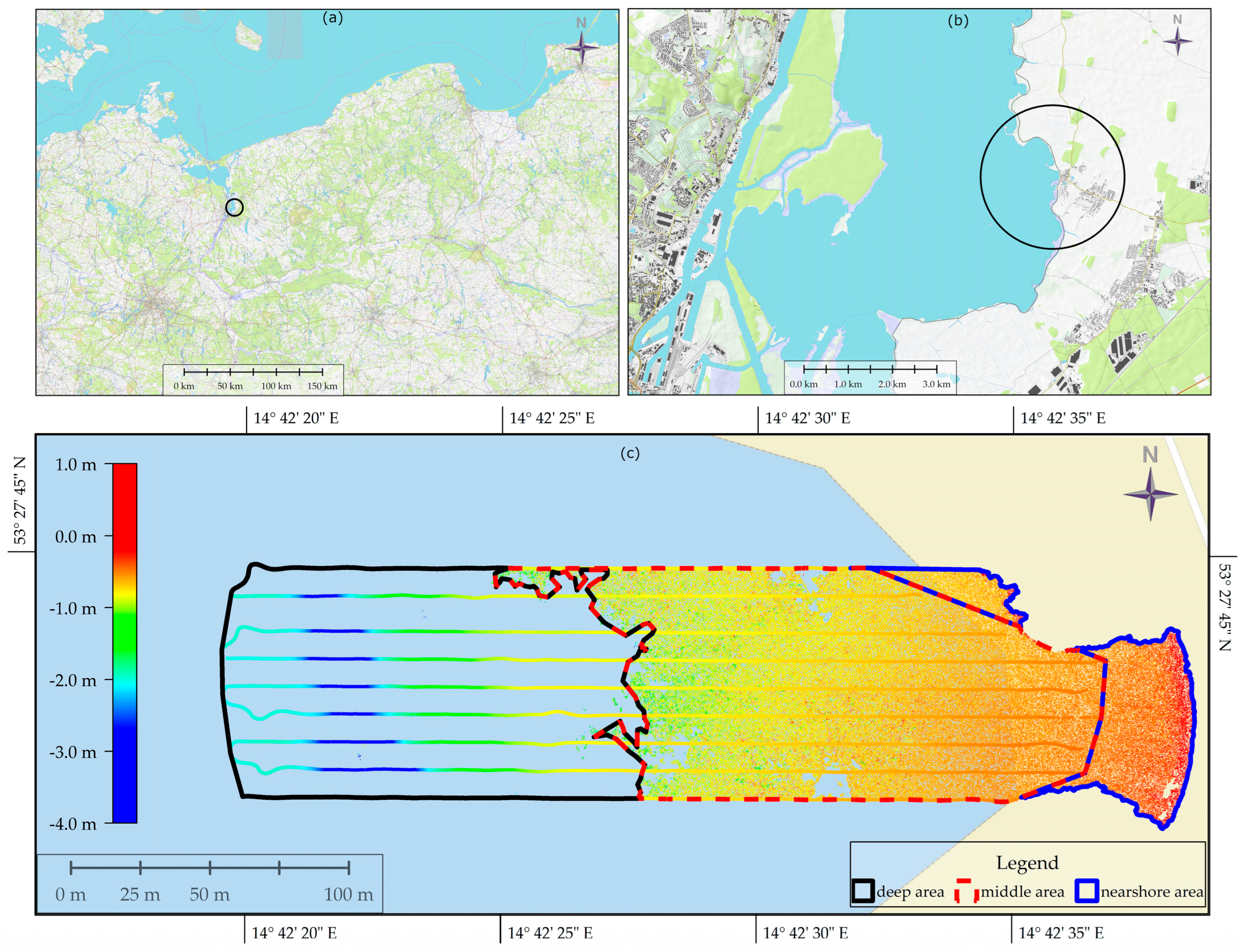
2. Study Area and Dataset Preprocessing
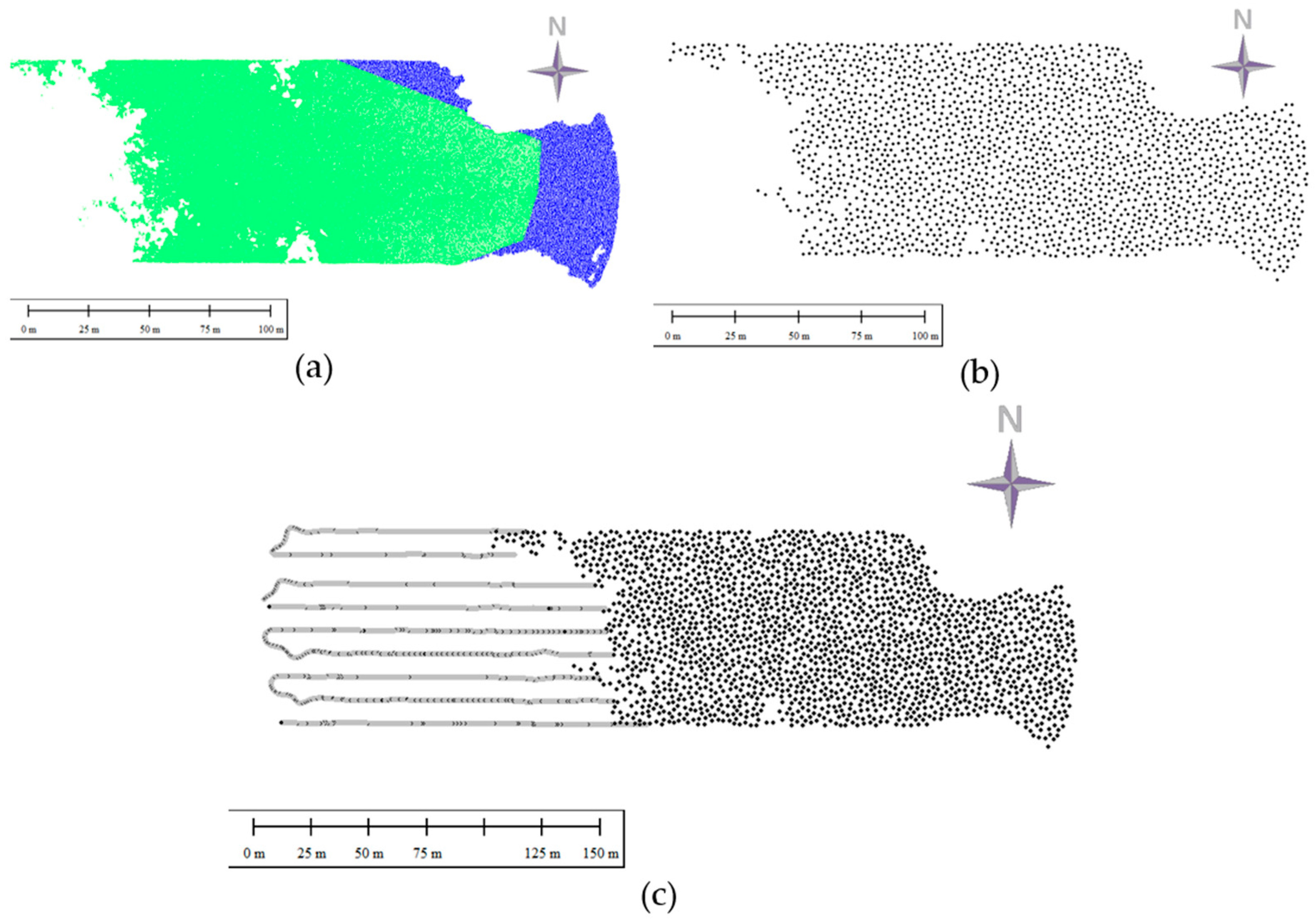
2.1. UAV Dataset—Photogrammetric Point Cloud
2.2. USV Dataset—Single-Beam Echosounder Data
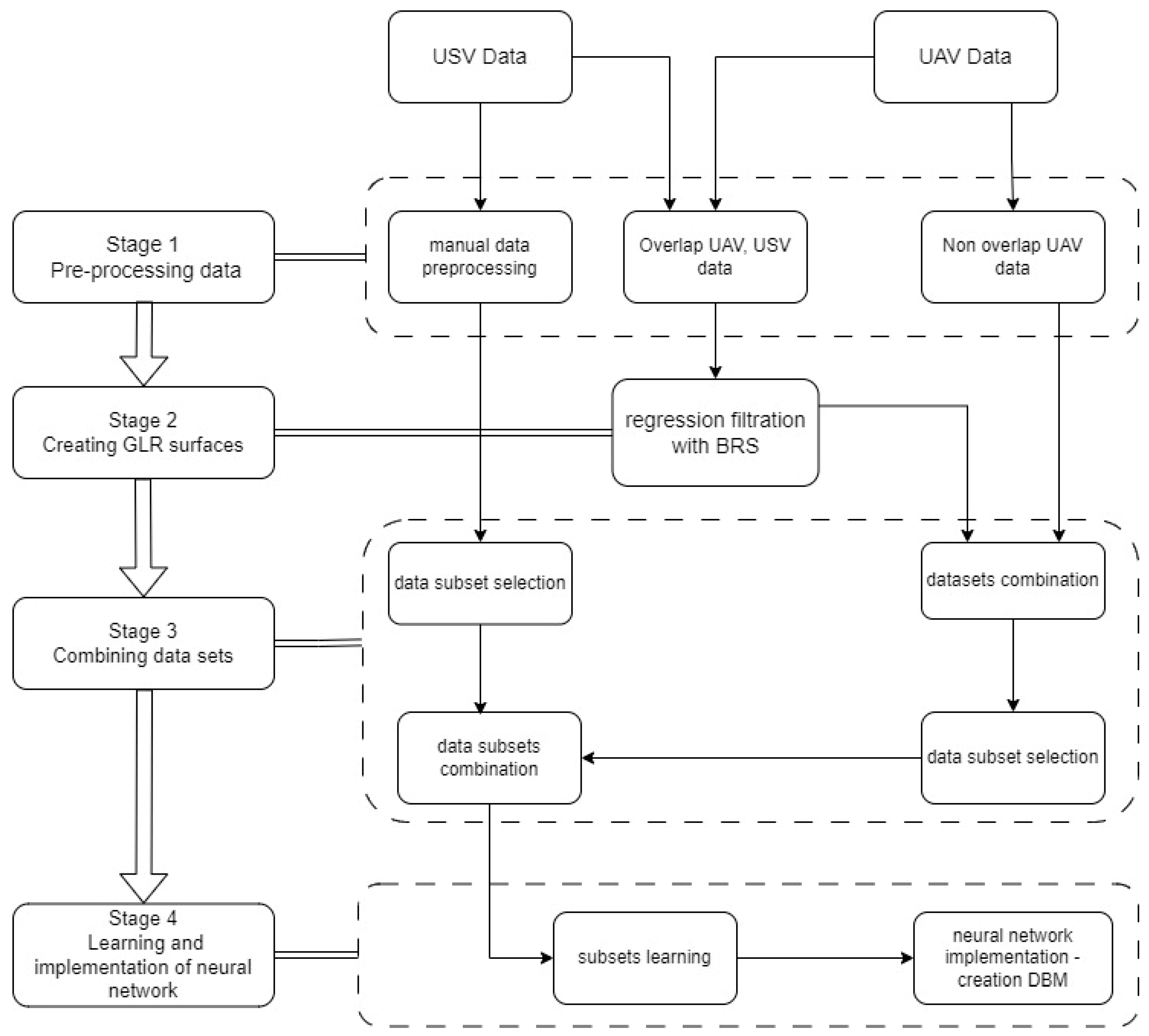
3. Methodology
3.1. Data Pre-Processing (Stage 1)
3.1.1. Pre-Processing Non-Overlap Photogrammetric Point Cloud Data
3.1.2. Pre-Processing Overlap Single-Beam Echosounder and Photogrammetric Point Cloud Data
- Reducing outlier observations;
- Reducing statistical sets;
- Filtering the reduced sets;
- Creating the DBM based on the MLP neural network.
3.1.3. Reduction in Outliers
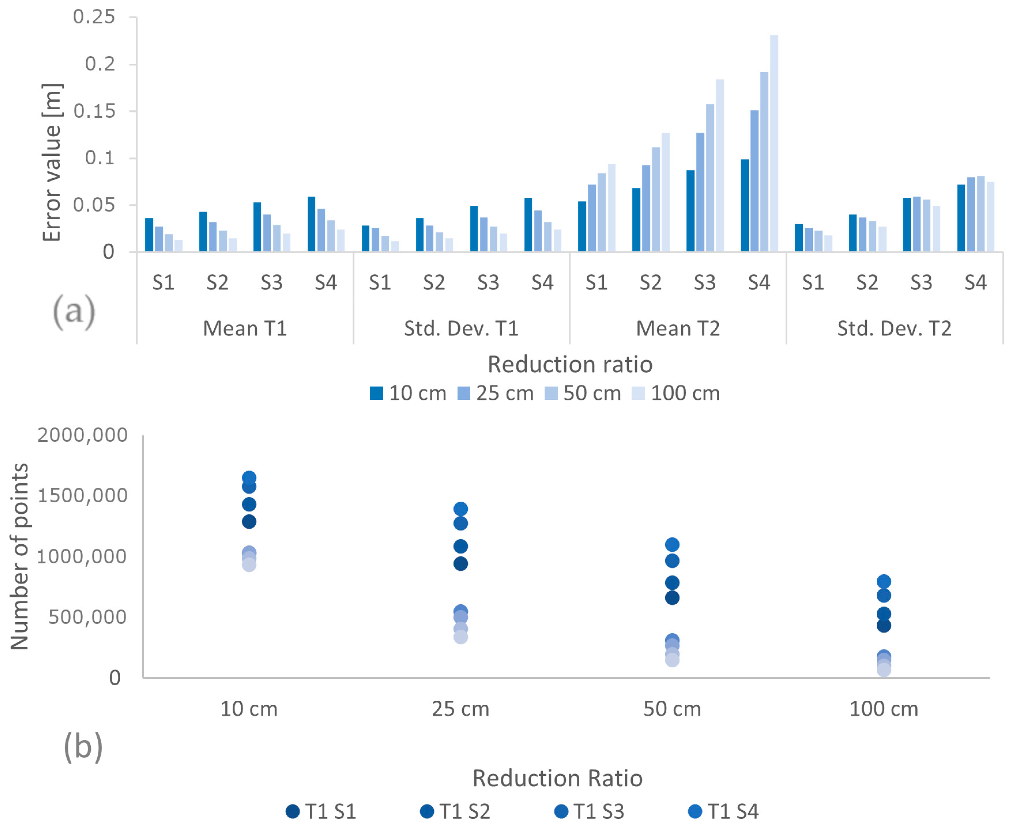
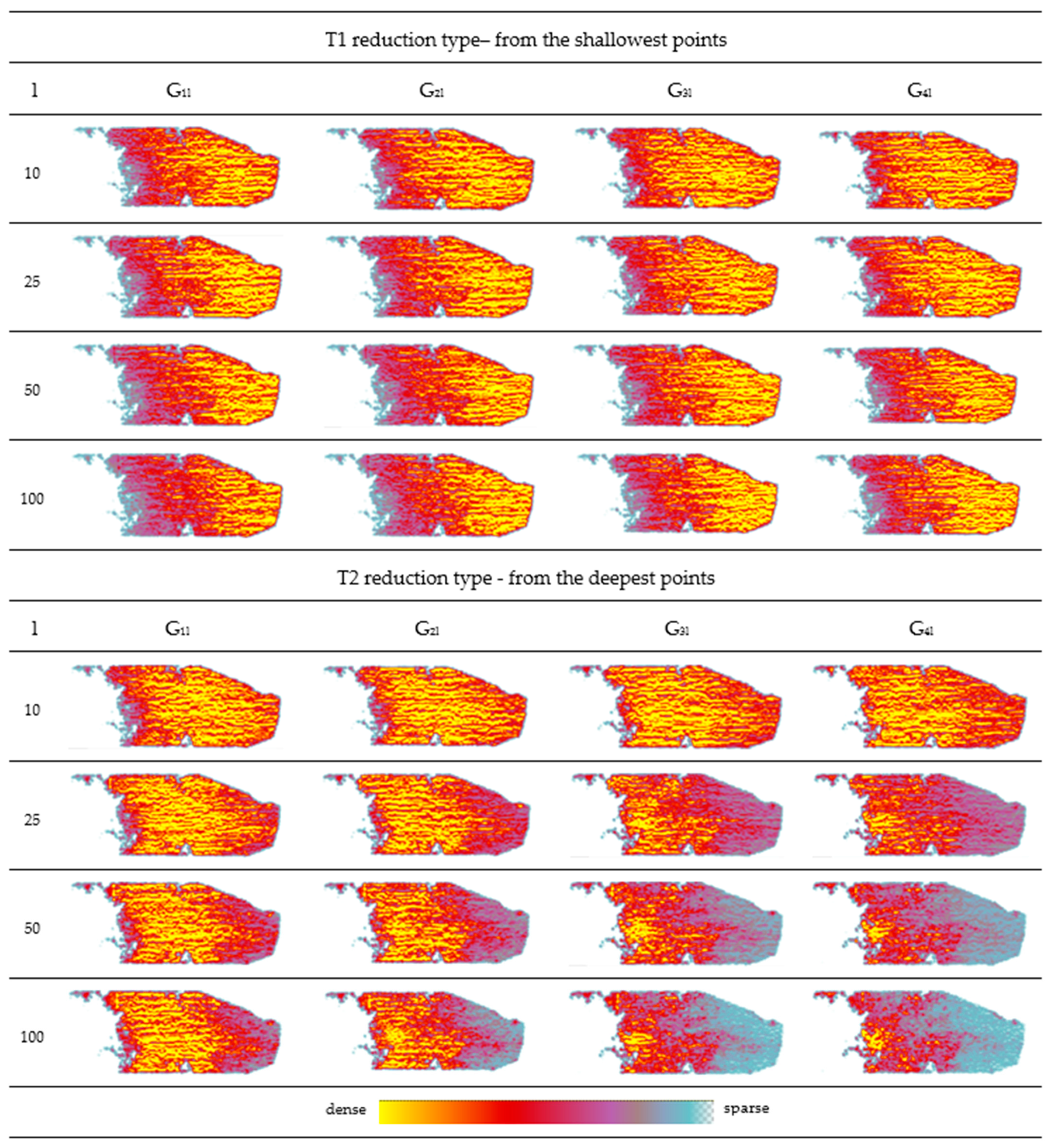
3.1.4. Analysis of Options for the Reduction in Statistical Sets
- The mean values of the DBRS assume higher values for the T2 reduction type;
- The mean values of the DBRS for T1 reduction take a maximum value of 0.06 m for set S4 with a reduction radius of 10 cm;
- For sets with a T1 reduction type, the values of the mean and standard deviation decrease in each statistical set; for T2 reductions, as the reduction ratio increases, the values of the mean significantly increase in the statistical sets, and the value of the standard deviation decreases in the statistical sets;
- T2 reduction type provides smaller datasets.
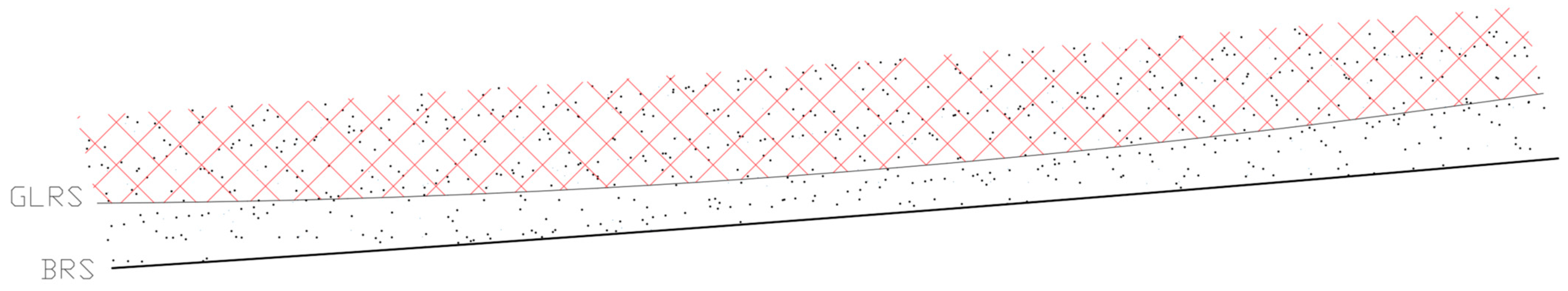
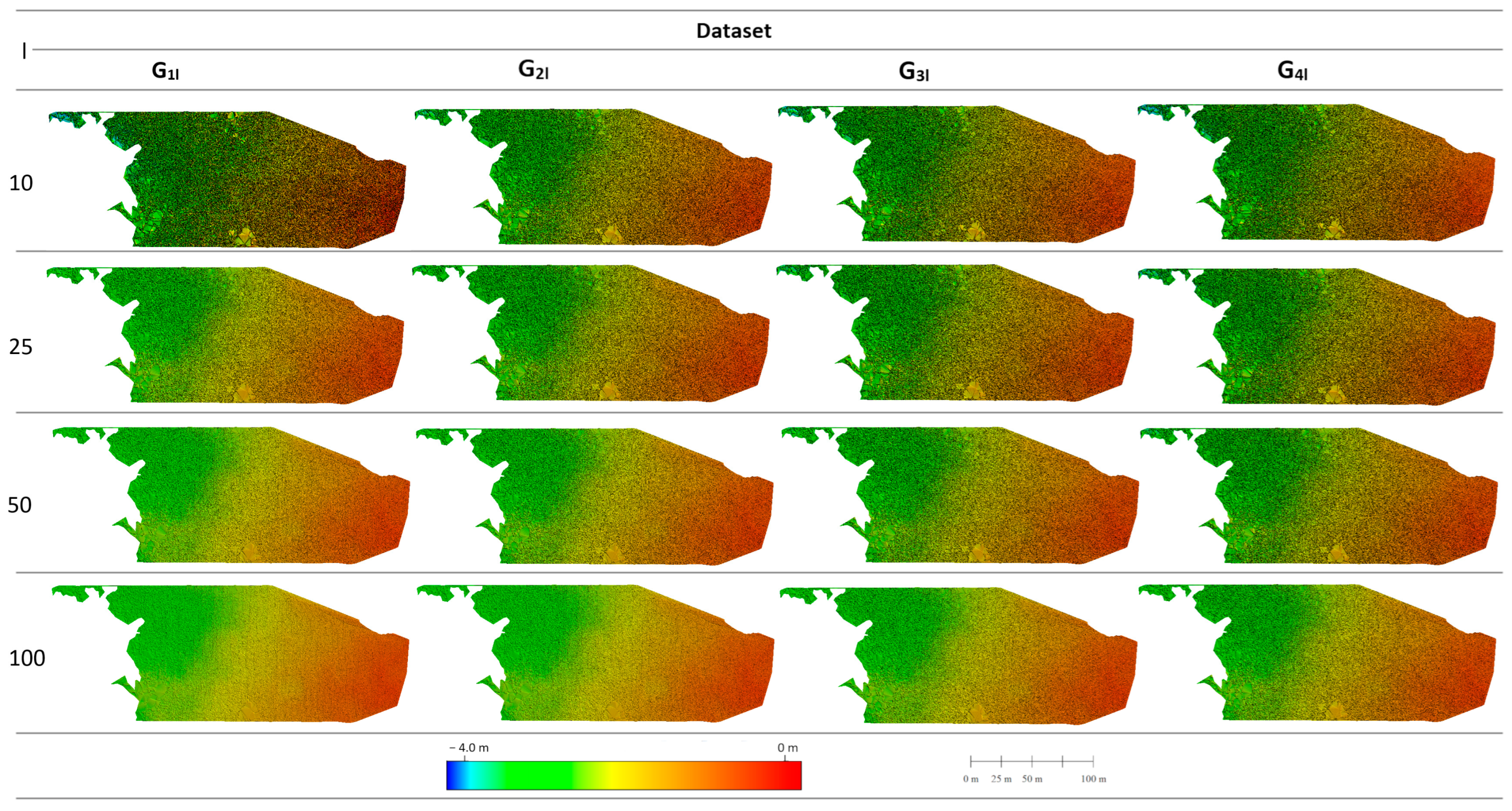
3.2. Creating GLR Surfaces (Stage 2)
3.3. Creation of Training Datasets (Stage 3)
3.4. Creation of Neural Digital Bathymetric Models (Stage 4)
4. Results
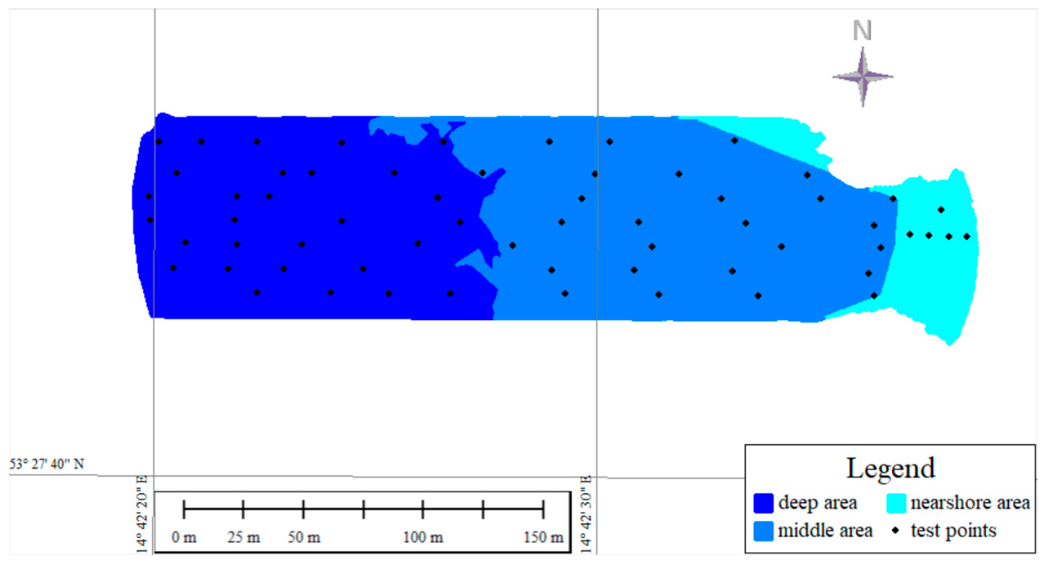
4.1. Test Dataset
4.2. Qualitative Assessment
4.3. Datasets for Results Analysis
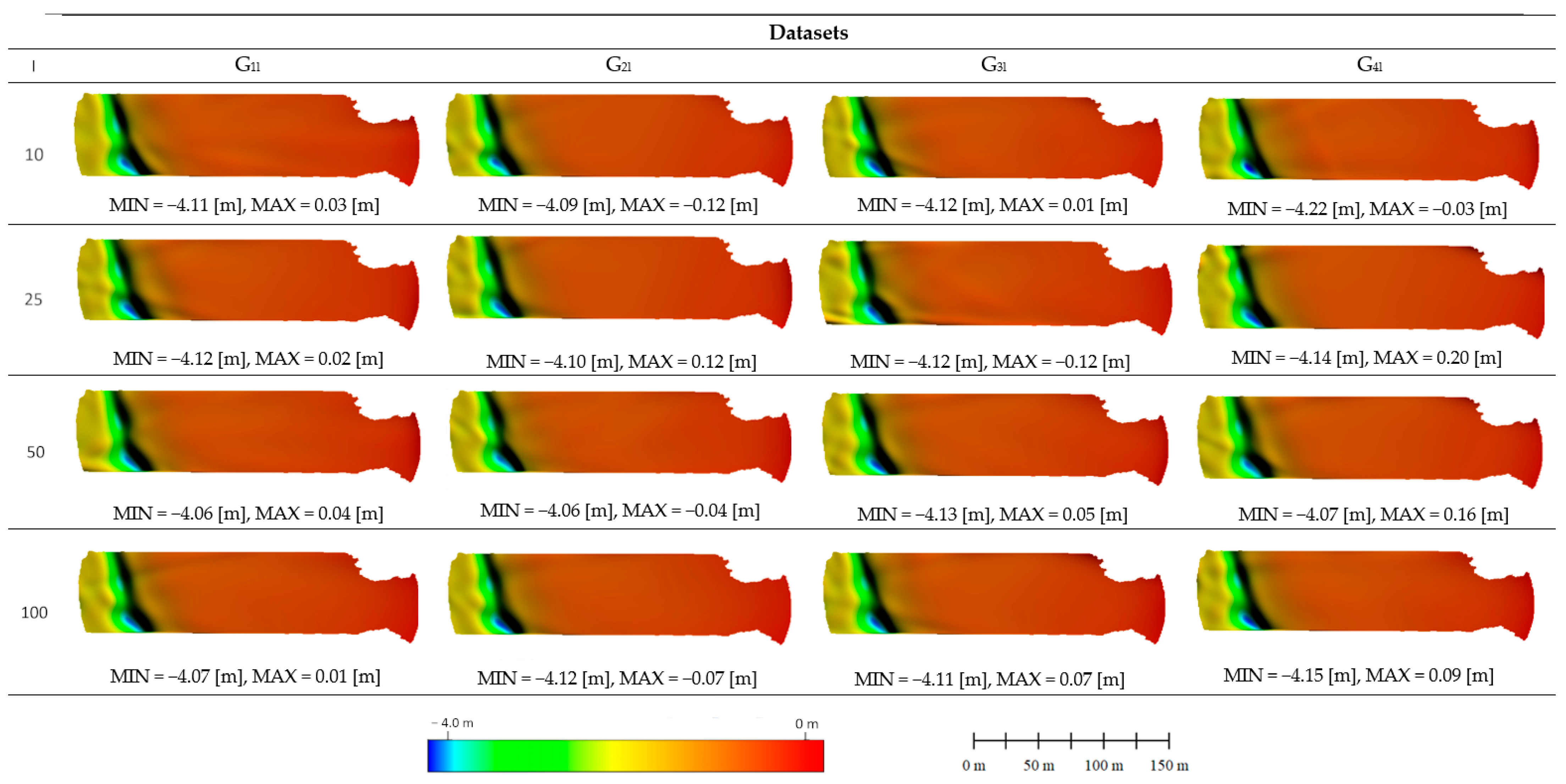
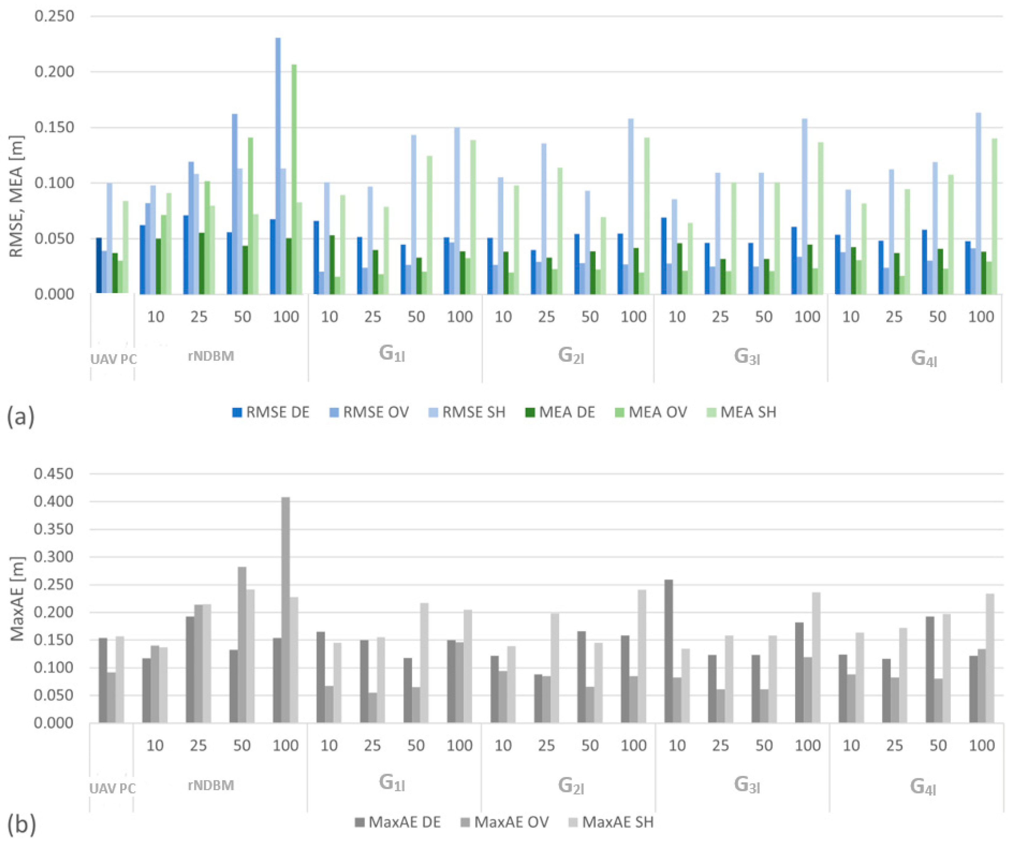
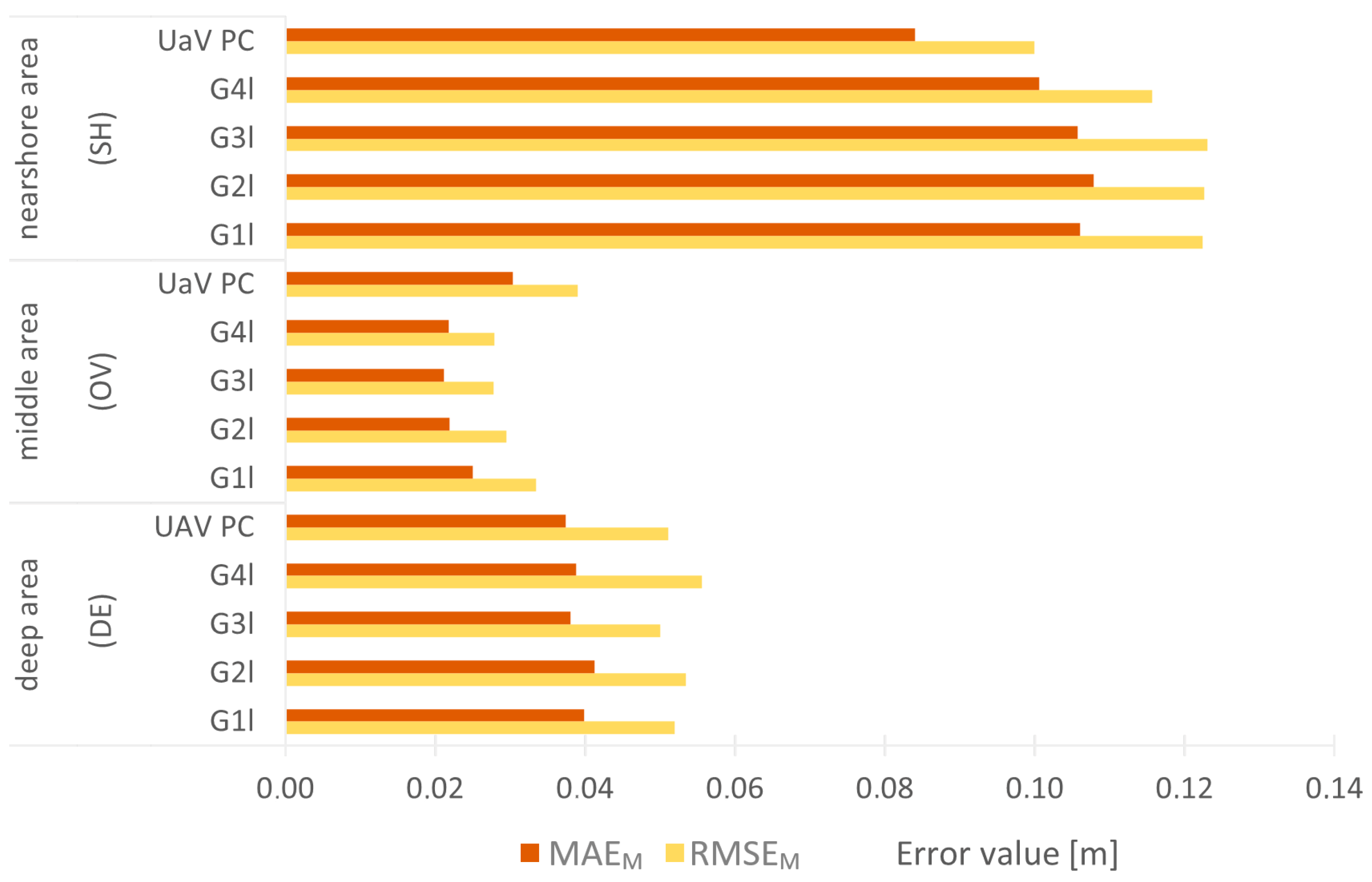
4.4. Results
5. Discussion
6. Conclusions
- The final accuracy of the calculated depths varies for each of the examined areas and depends on the input dataset;
- The filtering performed using the linear regression allowed the removal of outlier observations for the middle area;
- The reduction in the multi-million photogrammetric dataset is a most important step in creating a learning set;
- MLP neural networks allow depth calculation but may not preserve the true boundary values; the usefulness of such obtained models for navigation purposes may be limited, especially in shallow water areas.
Author Contributions
Funding
Institutional Review Board Statement
Informed Consent Statement
Data Availability Statement
Conflicts of Interest
Appendix A

References
- Mandlburger, G.; Pfennigbauer, M.; Schwarz, R.; Flöry, S.; Nussbaumer, L. Concept and Performance Evaluation of a Novel UAV-Borne Topo-Bathymetric LiDAR Sensor. Remote Sens. 2020, 12, 986. [Google Scholar] [CrossRef]
- Kasvi, E.; Salmela, J.; Lotsari, E.; Kumpula, T.; Lane, S.N. Comparison of Remote Sensing Based Approaches for Mapping Bathymetry of Shallow, Clear Water Rivers. Geomorphology 2019, 333, 180–197. [Google Scholar] [CrossRef]
- Bagheri, O.; Ghodsian, M.; Saadatseresht, M. Reach Scale Application of UAV+SfM Method in Shallow Rivers Hyperspatial Bathymetry. Int. Arch. Photogramm. Remote Sens. Spatial Inf. Sci. 2015, 40, 77–81. [Google Scholar] [CrossRef]
- Visser, F.; Woodget, A.; Skellern, A.; Forsey, J.; Warburton, J.; Johnson, R. An Evaluation of a Low-Cost Pole Aerial Photography (PAP) and Structure from Motion (SfM) Approach for Topographic Surveying of Small Rivers. Int. J. Remote Sens. 2019, 40, 9321–9351. [Google Scholar] [CrossRef]
- Dietrich, J.T. Bathymetric Structure-from-Motion: Extracting Shallow Stream Bathymetry from Multi-View Stereo Photogrammetry. Earth Surf. Process Landf. 2016, 42, 355–364. [Google Scholar] [CrossRef]
- David, C.G.; Kohl, N.; Casella, E.; Rovere, A.; Ballesteros, P.; Schlurmann, T. Structure-from-Motion on Shallow Reefs and Beaches: Potential and Limitations of Consumer-Grade Drones to Reconstruct Topography and Bathymetry. Coral Reefs 2021, 40, 835–851. [Google Scholar] [CrossRef]
- Lubczonek, J.; Kazimierski, W.; Zaniewicz, G.; Lacka, M. Methodology for Combining Data Acquired by Unmanned Surface and Aerial Vehicles to Create Digital Bathymetric Models in Shallow and Ultra-Shallow Waters. Remote Sens. 2022, 14, 105. [Google Scholar] [CrossRef]
- Starek, M.J.; Giessel, J. Fusion of Uas-Based Structure-from-Motion and Optical Inversion for Seamless Topo-Bathymetric Mapping. In Proceedings of the 2017 IEEE International Geoscience and Remote Sensing Symposium (IGARSS), Fort Worth, TX, USA, 2–28 July 2017; pp. 2999–3002. [Google Scholar]
- Agrafiotis, P.; Skarlatos, D.; Georgopoulos, A.; Karantzalos, K. Shallow Water Bathymetry Mapping from UAV Imagery Based on Machine Learning. Int. Arch. Photogramm. Remote Sens. Spatial Inf. 2019, 42, 9–16. [Google Scholar] [CrossRef]
- Del Savio, A.A.; Luna Torres, A.; Vergara Olivera, M.A.; Llimpe Rojas, S.R.; Urday Ibarra, G.T.; Neckel, A. Using UAVs and Photogrammetry in Bathymetric Surveys in Shallow Waters. Appl. Sci. 2023, 13, 3420. [Google Scholar] [CrossRef]
- Rossi, L.; Mammi, I.; Pelliccia, F. UAV-Derived Multispectral Bathymetry. Remote Sens. 2020, 12, 3897. [Google Scholar] [CrossRef]
- Stumpf, R.P.; Holderied, K.; Sinclair, M. Determination of Water Depth with High-Resolution Satellite Imagery over Variable Bottom Types. Limnol. Oceanogr. 2003, 48, 547–556. [Google Scholar] [CrossRef]
- Lyzenga, D.R. Passive Remote Sensing Techniques for Mapping Water Depth and Bottom Features. Appl. Opt. 1978, 17, 379–383. [Google Scholar] [CrossRef] [PubMed]
- Gentile, V.; Mróz, M.; Spitoni, M.; Lejot, J.; Piégay, H.; Demarchi, L. Bathymetric Mapping of Shallow Rivers with UAV Hyperspectral Data. In Proceedings of the Fifth International Conference on Telecommunications and Remote Sensing, Milan, Italy, 10–11 October 2016; pp. 43–49. [Google Scholar]
- Hodúl, M.; Bird, S.; Knudby, A.; Chénier, R. Satellite Derived Photogrammetric Bathymetry. ISPRS J. Photogramm. Remote Sens. 2018, 142, 268–277. [Google Scholar] [CrossRef]
- Amini, L.; Kakroodi, A.A. Bathymetry of Shallow Coastal Environment Using Multi-Spectral Passive Data under Rapid Sea–Level Change. J. Sea Res. 2023, 194, 102403. [Google Scholar] [CrossRef]
- Ashphaq, M.; Srivastava, P.K.; Mitra, D. Review of Near-Shore Satellite Derived Bathymetry: Classification and Account of Five Decades of Coastal Bathymetry Research. J. Ocean. Eng. Sci. 2021, 6, 340–359. [Google Scholar] [CrossRef]
- Szafarczyk, A.; Toś, C. The Use of Green Laser in LiDAR Bathymetry: State of the Art and Recent Advancements. Sensors 2023, 23, 292. [Google Scholar] [CrossRef]
- Wang, D.; Xing, S.; He, Y.; Yu, J.; Xu, Q.; Li, P. Evaluation of a New Lightweight UAV-Borne Topo-Bathymetric LiDAR for Shallow Water Bathymetry and Object Detection. Sensors 2022, 22, 1379. [Google Scholar] [CrossRef]
- Janowski, L.; Wroblewski, R.; Rucinska, M.; Kubowicz-Grajewska, A.; Tysiac, P. Automatic Classification and Mapping of the Seabed Using Airborne LiDAR Bathymetry. Eng. Geol. 2022, 301, 106615. [Google Scholar] [CrossRef]
- Soeksmantono, B.; Utama, Y.P.; Syaifudin, F. Utilization of Airborne Topo-Bathymetric LiDAR Technology for Coastline Determination in Western Part of Java Island. In Proceedings of the IOP Conference Series: Earth and Environmental Science; IOP Publishing Ltd.: Bristol, UK, 2021; Volume 925. [Google Scholar]
- Lee, Z.; Shangguan, M.; Garcia, R.A.; Lai, W.; Lu, X.; Wang, J.; Yan, X. Confidence Measure of the Shallow-Water Bathymetry Map Obtained through the Fusion of Lidar and Multiband Image Data. J. Remote Sens. 2021, 2021, 1–16. [Google Scholar] [CrossRef]
- Tysiac, P. Bringing Bathymetry Lidar to Coastal Zone Assessment: A Case Study in the Southern Baltic. Remote Sens. 2020, 12, 3740. [Google Scholar] [CrossRef]
- Andersen, M.S.; Gergely, Á.; Al-Hamdani, Z.; Steinbacher, F.; Larsen, L.R.; Ernstsen, V.B. Processing and Performance of Topobathymetric Lidar Data for Geomorphometric and Morphological Classification in a High-Energy Tidal Environment. Hydrol. Earth Syst. Sci. 2017, 21, 43–63. [Google Scholar] [CrossRef]
- Quadros, N.D.; Collier, P.A.; Fraser, C.S. Integration of bathymetric and topographic LiDAR: A preliminary investigation. Remote Sens. Spat. Inf. Sci. 2008, 37, 1299–1304. [Google Scholar]
- Alvarez, L.V.; Moreno, H.A.; Segales, A.R.; Pham, T.G.; Pillar-Little, E.A.; Chilson, P.B. Merging Unmanned Aerial Systems (UAS) Imagery and Echo Soundings with an Adaptive Sampling Technique for Bathymetric Surveys. Remote Sens. 2018, 10, 1362. [Google Scholar] [CrossRef]
- Zhang, C. Applying Data Fusion Techniques for Benthic Habitat Mapping and Monitoring in a Coral Reef Ecosystem. ISPRS J. Photogramm. Remote Sens. 2015, 104, 213–223. [Google Scholar] [CrossRef]
- Yang, H.; Guo, H.; Dai, W.; Nie, B.; Qiao, B.; Zhu, L. Bathymetric Mapping and Estimation of Water Storage in a Shallow Lake Using a Remote Sensing Inversion Method Based on Machine Learning. Int. J. Digit. Earth 2022, 15, 789–812. [Google Scholar] [CrossRef]
- Forfinski-Sarkozi, N.A.; Parrish, C.E. Active-Passive Spaceborne Data Fusion for Mapping Nearshore Bathymetry. Photogramm. Eng. Remote Sens. 2019, 85, 281–295. [Google Scholar] [CrossRef]
- Yunus, A.P.; Dou, J.; Song, X.; Avtar, R. Improved Bathymetric Mapping of Coastal and Lake Environments Using Sentinel-2 and Landsat-8 Images. Sensors 2019, 19, 2788. [Google Scholar] [CrossRef]
- Villalpando, F.; Tuxpan, J.; Ramos-Leal, J.A.; Marin, A.E. Towards of Multi-Source Data Fusion Framework of Geo-Referenced and Non-Georeferenced Data: Prospects for Use in Surface Water Bodies. Geocarto Int. 2023, 2172215. [Google Scholar] [CrossRef]
- Noman, J.; Cassol, W.N.; Daniel, S.; Pham Van Bang, D. Bathymetric Data Integration Approach to Study Bedforms in the Estuary of the Saint-Lawrence River. Front. Remote Sens. 2023, 4, 1125898. [Google Scholar] [CrossRef]
- Joe, H.; Cho, H.; Sung, M.; Kim, J.; Yu, S.c. Sensor Fusion of Two Sonar Devices for Underwater 3D Mapping with an AUV. Auton. Robot. 2021, 45, 543–560. [Google Scholar] [CrossRef]
- Cooper, I.; Hotchkiss, R.H.; Williams, G.P. Extending Multi-Beam Sonar with Structure from Motion Data of Shorelines for Complete Pool Bathymetry of Reservoirs. Remote Sens. 2021, 13, 35. [Google Scholar] [CrossRef]
- Sotelo-Torres, F.; Alvarez, L.V.; Roberts, R.C. An Unmanned Surface Vehicle (USV): Development of an Autonomous Boat with a Sensor Integration System for Bathymetric Surveys. Sensors 2023, 23, 4420. [Google Scholar] [CrossRef]
- Alevizos, E.; Oikonomou, D.; Argyriou, A.V.; Alexakis, D.D. Fusion of Drone-Based RGB and Multi-Spectral Imagery for Shallow Water Bathymetry Inversion. Remote Sens. 2022, 14, 1127. [Google Scholar] [CrossRef]
- Chormański, J.; Nowicka, B.; Wieckowski, A.; Ciupak, M.; Jóźwiak, J.; Figura, T. Coupling of Dual Channel Waveform Als and Sonar for Investigation of Lake Bottoms and Shore Zones. Remote Sens. 2021, 13, 1833. [Google Scholar] [CrossRef]
- Ferreira, F.; Machado, D.; Ferri, G.; Dugelay, S.; Potter, J. Underwater Optical and Acoustic Imaging: A Time for Fusion? A Brief Overview of the State-of-the-Art. In Proceedings of the OCEANS 2016 MTS/IEEE Monterey, Monterey, CA, USA, 19–23 September 2016; pp. 1–6. [Google Scholar]
- Włodarczyk-Sielicka, M.; Bodus-Olkowska, I.; Łącka, M. The Process of Modelling the Elevation Surface of a Coastal Area Using the Fusion of Spatial Data from Different Sensors. Oceanologia 2022, 64, 22–34. [Google Scholar] [CrossRef]
- Lubczonek, J.; Wlodarczyk-Sielicka, M.; Lacka, M.; Zaniewicz, G. Methodology for Developing a Combined Bathymetric and Topographic Surface Model Using Interpolation and Geodata Reduction Techniques. Remote Sens. 2021, 13, 4427. [Google Scholar] [CrossRef]
- Genchi, S.A.; Vitale, A.J.; Perillo, G.M.E.; Seitz, C.; Delrieux, C.A. Mapping Topobathymetry in a Shallow Tidal Environment Using Low-Cost Technology. Remote Sens. 2020, 12, 1394. [Google Scholar] [CrossRef]
- Sonogashira, M.; Shonai, M.; Iiyama, M. High-Resolution Bathymetry by Deep-Learning-Based Image Superresolution. PLoS ONE 2020, 15, e0235487. [Google Scholar] [CrossRef]
- Slocum, R.K.; Parrish, C.E.; Simpson, C.H. Combined Geometric-Radiometric and Neural Network Approach to Shallow Bathymetric Mapping with UAS Imagery. ISPRS J. Photogramm. Remote Sens. 2020, 169, 351–363. [Google Scholar] [CrossRef]
- Liu, S.; Wang, L.; Liu, H.; Su, H.; Li, X.; Zheng, W. Deriving Bathymetry from Optical Images with a Localized Neural Network Algorithm. IEEE Trans. Geosci. Remote Sens. 2018, 56, 5334–5342. [Google Scholar] [CrossRef]
- Kaloop, M.R.; El-Diasty, M.; Hu, J.W.; Zarzoura, F. Hybrid Artificial Neural Networks for Modeling Shallow-Water Bathymetry via Satellite Imagery. IEEE Trans. Geosci. Remote Sens. 2022, 60, 5403811. [Google Scholar] [CrossRef]
- Al Najar, M.; Thoumyre, G.; Bergsma, E.W.J.; Almar, R.; Benshila, R.; Wilson, D.G. Satellite Derived Bathymetry Using Deep Learning. Mach. Learn. 2023, 112, 1107–1130. [Google Scholar] [CrossRef]
- ArcGIS Pro Help, Generalized Linear Regression. Available online: https://pro.arcgis.com/en/pro-app/latest/tool-reference/spatial-statistics/generalized-linear-regression.htm (accessed on 10 September 2023).
- Becker, C.; Rosinskaya, E.; Häni, N.; d’Angelo, E.; Strecha, C. Classification of Aerial Photogrammetric 3D Point Clouds. Photogramm. Eng. Remote Sens. 2018, 84, 287–295. [Google Scholar] [CrossRef]
- ArcGIS Pro Help, Reduce Point Density. Available online: https://pro.arcgis.com/en/pro-app/latest/tool-reference/maritime/reduce-point-density.htm (accessed on 10 September 2023).
- ArcGIS Pro Help, Create Random Points (Data Management). Available online: https://pro.arcgis.com/en/pro-app/latest/tool-reference/data-management/create-random-points.htm (accessed on 10 September 2023).
- Chuchro, M. Environmental Data Analysis Using Data Mining Methods (Analiza danych środowiskowych metodami eksploracji danych). Stud. Inform. 2011, 32, 417–428. (in Polish). [Google Scholar]
- Broyden, C.G. The convergence of a class of double-rank minimization algorithms 1. General Considerations. IMA J. Appl. Math. 1970, 6, 76–90. [Google Scholar] [CrossRef]
- Fletcher, R. A New Approach to Variable Metric Algorithms. Comput. J. 1970, 13, 317–322. [Google Scholar] [CrossRef]
- Goldfarb, D. A family of variable-metric methods derived by variational means. Math. Comput. 1970, 24, 23–26. [Google Scholar] [CrossRef]
- Shanno, D.F. Conditioning of quasi-Newton methods for function minimization. Math. Comput. 1970, 24, 647–656. [Google Scholar] [CrossRef]
- StatSoft. Electronic Statistics Handbook. (In Polish: Elektroniczny Podręcznik Statystyki PL), Krakow. 2006. Available online: http://www.statsoft.pl/textbook/stathome.html (accessed on 10 September 2023).
- Lubczonek, J.; Zaniewicz, G. Application of Filtering Techniques to Smooth a Surface of Hybrid Digital Bathymetric Model. Remote Sens. 2023, 15, 4737. [Google Scholar] [CrossRef]
- International Hydrographic Organization (IHO). IHO Standards for Hydrographic Surveys, 6th ed.; International Hydrographic Bureau: Monaco, Monaco, 2020. [Google Scholar]


| Input Dataset | Reduction Ratio | ||||
|---|---|---|---|---|---|
| 10 cm | 25 cm | 50 cm | 100 cm | ||
| Number of points | 438,843 | 183,204 | 45,556 | 12,868 | 3221 |
| Maximum value (m) | −1.7 | −1.7 | −1.1 | −1.0 | −0.7 |
| Mean value (m) | −0.4 | −0.4 | −0.4 | −0.4 | −0.3 |
| Standard deviation (m) | 0.16 | 0.16 | 0.16 | 0.17 | 0.17 |
| Dataset | S1 | S2 | S3 | S4 |
|---|---|---|---|---|
| Number of points | 1,679,496 | 1,836,494 | 1,972,763 | 2,021,762 |
| Max value (m) | 0.12 | 0.16 | 0.25 | 0.335 |
| Mean value (m) | 0.04 | 0.05 | 0.06 | 0.07 |
| Standard deviation (m) | 0.03 | 0.04 | 0.05 | 0.06 |
| Reduction Ratio (l) [cm] | Neural Network Name | Quality (Learning) | Quality (Testing) | Quality (Validation) | Learning Algorithm | Error Function | |
|---|---|---|---|---|---|---|---|
| G1l | 10 | MLP 2-30-1 | 0.997579 | 0.997687 | 0.997110 | BFGS 1286 | SOS |
| 25 | MLP 2-28-1 | 0.998315 | 0.998366 | 0.998245 | BFGS 1115 | SOS | |
| 50 | MLP 2-29-1 | 0.998106 | 0.997959 | 0.997642 | BFGS 1516 | SOS | |
| 100 | MLP 2-28-1 | 0.998130 | 0.997679 | 0.998229 | BFGS 1075 | SOS | |
| G2l | 10 | MLP 2-30-1 | 0.997940 | 0.998245 | 0.998116 | BFGS 844 | SOS |
| 25 | MLP 2-28-1 | 0.998107 | 0.998055 | 0.998017 | BFGS 1074 | SOS | |
| 50 | MLP 2-30-1 | 0.998215 | 0.998124 | 0.998015 | BFGS 1132 | SOS | |
| 100 | MLP 2-29-1 | 0.998046 | 0.998050 | 0.998328 | BFGS 944 | SOS | |
| G3l | 10 | MLP 2-30-1 | 0.997976 | 0.998204 | 0.997950 | BFGS 1370 | SOS |
| 25 | MLP 2-29-1 | 0.998249 | 0.998507 | 0.997931 | BFGS 1227 | SOS | |
| 50 | MLP 2-28-1 | 0.998282 | 0.997973 | 0.997875 | BFGS 1307 | SOS | |
| 100 | MLP 2-30-1 | 0.998332 | 0.998146 | 0.998344 | BFGS 1126 | SOS | |
| G4l | 10 | MLP 2-27-1 | 0.997582 | 0.997774 | 0.997705 | BFGS 1113 | SOS |
| 25 | MLP 2-30-1 | 0.998351 | 0.998232 | 0.998221 | BFGS 1399 | SOS | |
| 50 | MLP 2-28-1 | 0.998390 | 0.998508 | 0.998470 | BFGS 1323 | SOS | |
| 100 | MLP 2-30-1 | 0.998217 | 0.998513 | 0.998259 | BFGS 1428 | SOS |
Disclaimer/Publisher’s Note: The statements, opinions and data contained in all publications are solely those of the individual author(s) and contributor(s) and not of MDPI and/or the editor(s). MDPI and/or the editor(s) disclaim responsibility for any injury to people or property resulting from any ideas, methods, instructions or products referred to in the content. |
© 2023 by the authors. Licensee MDPI, Basel, Switzerland. This article is an open access article distributed under the terms and conditions of the Creative Commons Attribution (CC BY) license (https://creativecommons.org/licenses/by/4.0/).
Share and Cite
Łącka, M.; Łubczonek, J. Methodology for Creating a Digital Bathymetric Model Using Neural Networks for Combined Hydroacoustic and Photogrammetric Data in Shallow Water Areas. Sensors 2024, 24, 175. https://doi.org/10.3390/s24010175
Łącka M, Łubczonek J. Methodology for Creating a Digital Bathymetric Model Using Neural Networks for Combined Hydroacoustic and Photogrammetric Data in Shallow Water Areas. Sensors. 2024; 24(1):175. https://doi.org/10.3390/s24010175
Chicago/Turabian StyleŁącka, Małgorzata, and Jacek Łubczonek. 2024. "Methodology for Creating a Digital Bathymetric Model Using Neural Networks for Combined Hydroacoustic and Photogrammetric Data in Shallow Water Areas" Sensors 24, no. 1: 175. https://doi.org/10.3390/s24010175