
Microbiological Quality Estimation of Meat Using Deep CNNs on Embedded Hardware Systems
 , and
, and
Abstract
:1. Introduction
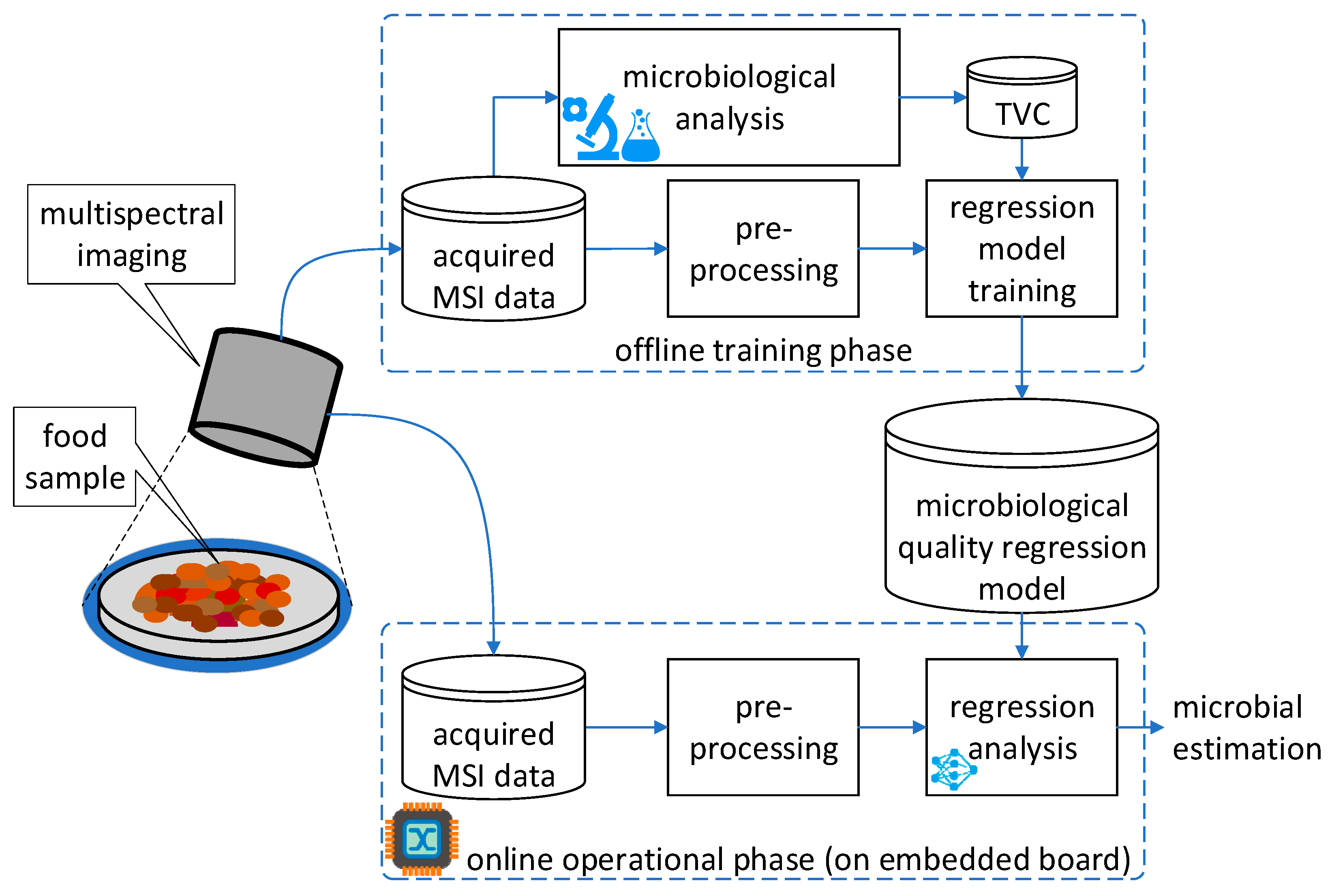
2. System Architecture
2.1. Acquisition of Food Imaging Data and Estimation of Microbial Population
2.2. Offline Training Phase
2.3. Online Operation Phase
3. Experimental Setup
3.1. Evaluation Datasets
3.2. Models
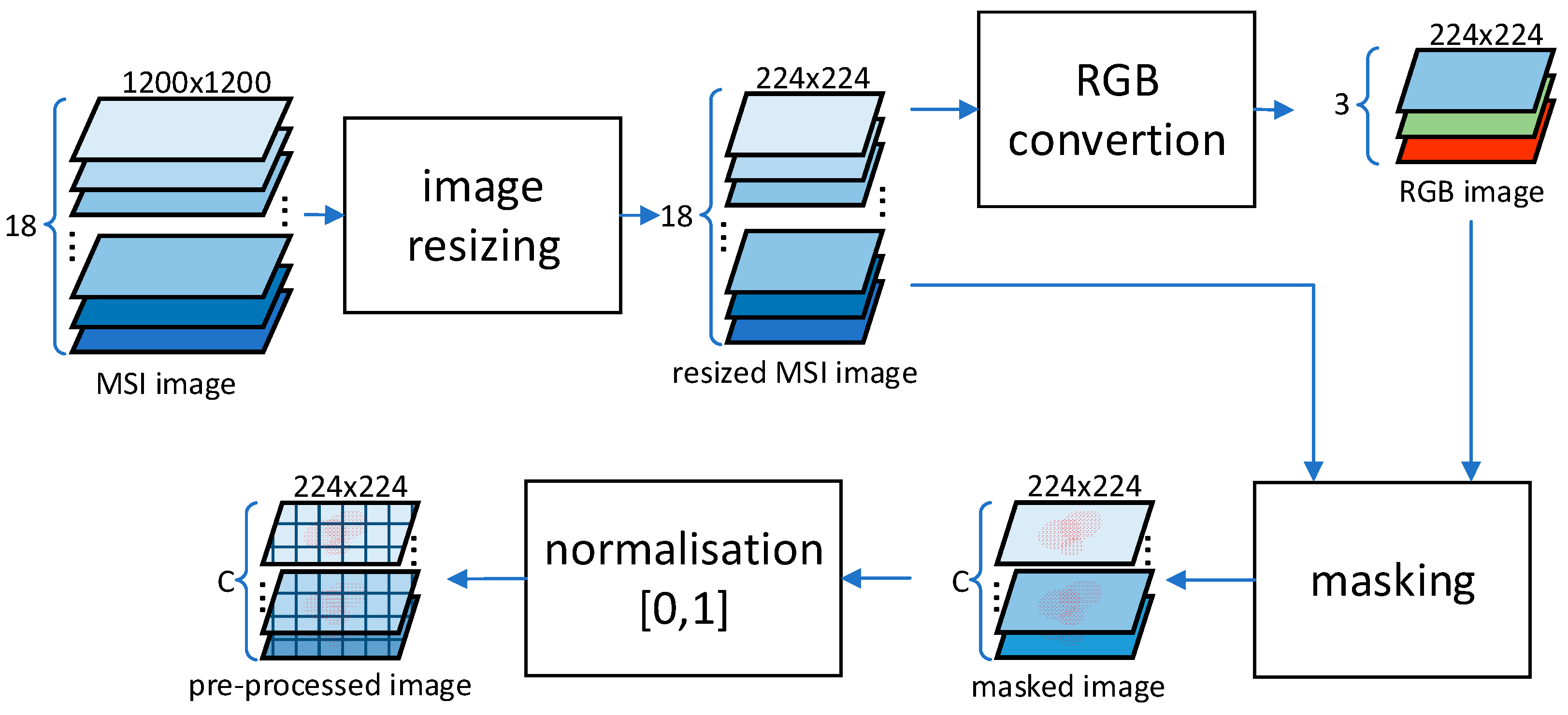
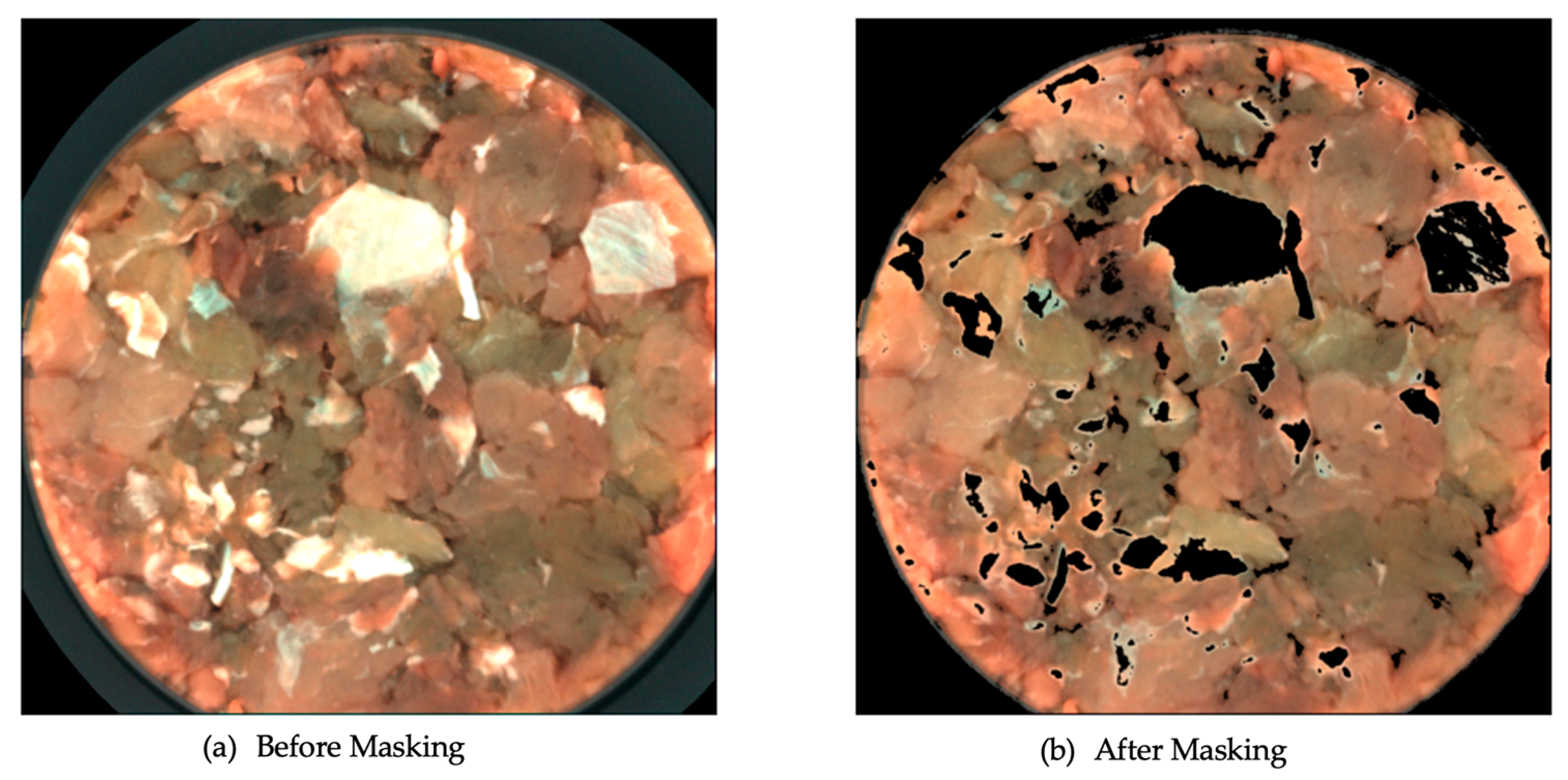
3.2.1. K-Means Masking
3.2.2. CNN Regression Models
3.3. Embedded Systems
- RP4_64bit (Raspberry Pi 4 Model B 8 GB)
- 2.
- NCS2 (Raspberry Pi 4 Model B 4 GB + Intel Neural Compute Stick 2)
- 3.
- IMX8P (NXP i.MX 8M Plus)
- 4.
- Nano (NVIDIA Jetson Nano)
- 5.
- XavierNX (NVIDIA Jetson Xavier NX)
- 6.
- Ultra96 (Avnet Ultra96-V1)
- 7.
- KV260 (Xilinx Kria KV260 Starter Kit)
4. Experimental Results
4.1. Microbial Population Estimation
4.1.1. Accuracy Metrics
4.1.2. CNN-Based Microbial Population Estimation
4.1.3. CNN Performance with Data Quantization
4.2. Embedded Systems Performance
4.2.1. Hardware Performance Metrics
- Latency: Execution time from start to finish of a specific stage. To accurately extract this measurement, the application was run multiple times, and the average latency time was calculated for each stage. The overall test time was at least 30 s; apart from the target application process, other OS processes use the hardware resources too (such as CPU cores, cache memory, etc.), which may add noise to the experimental results. Stages of interest included loading MSI data, pre-processing, and model inference.
- Throughput
- 3.
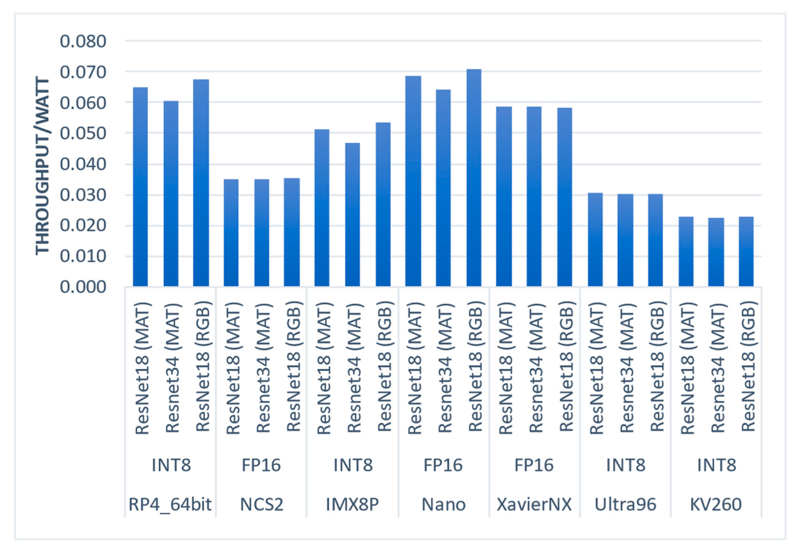
- Efficiency (Throughput/Watt)
- 4.
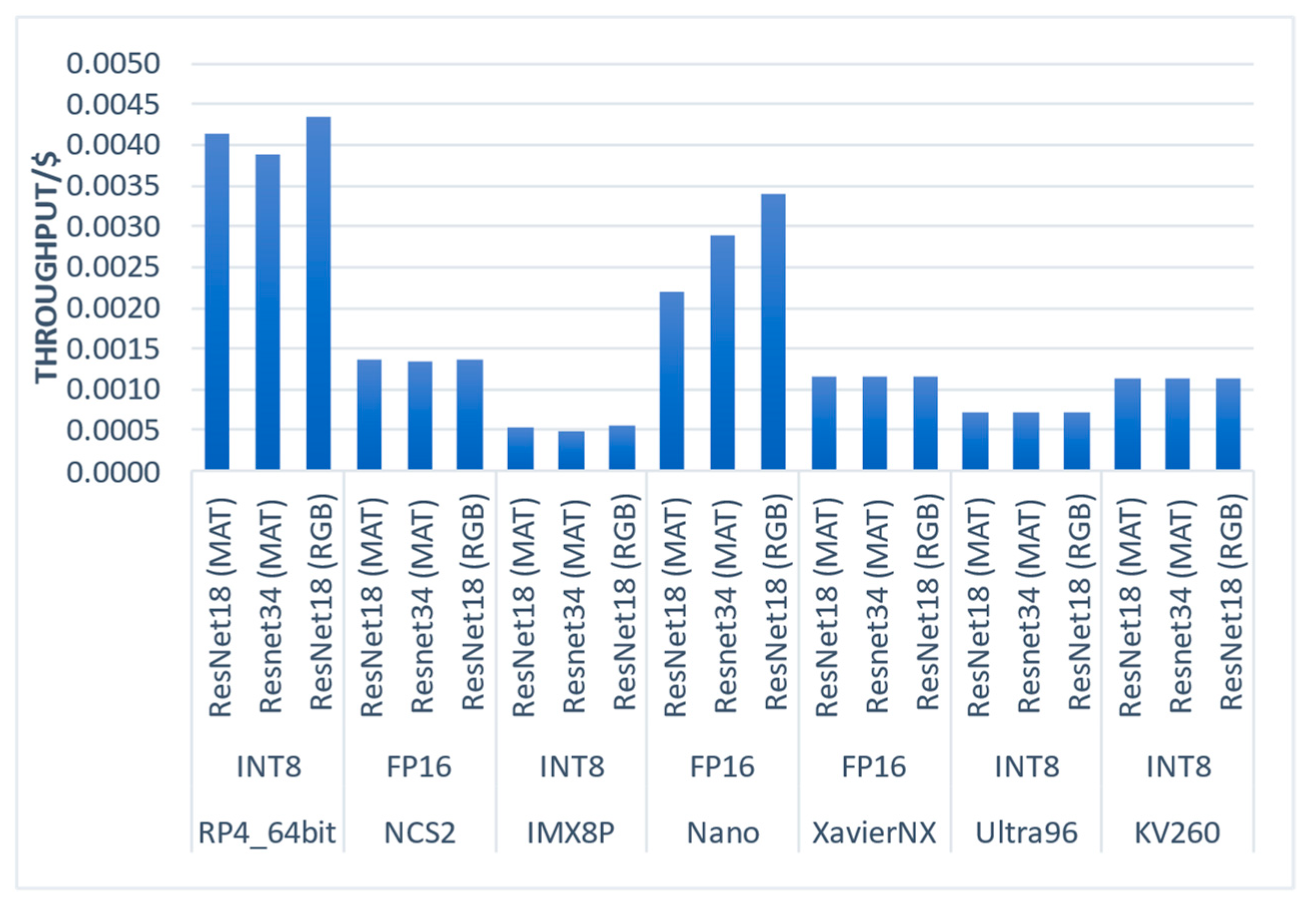
- Value (Throughput/Cost)
4.2.2. Hardware Evaluation Results
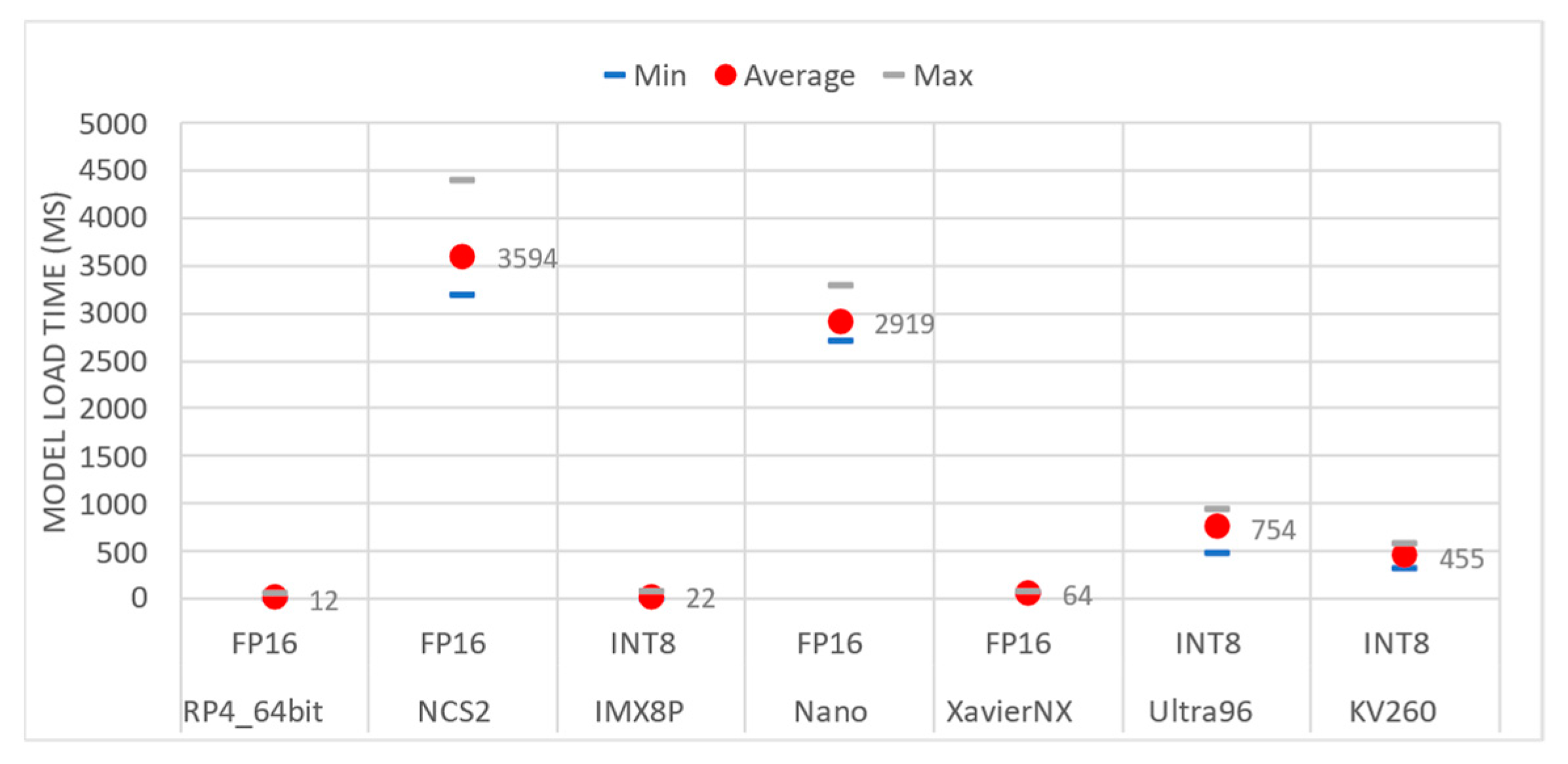
- Load CNN Model (Latency)
- 2.
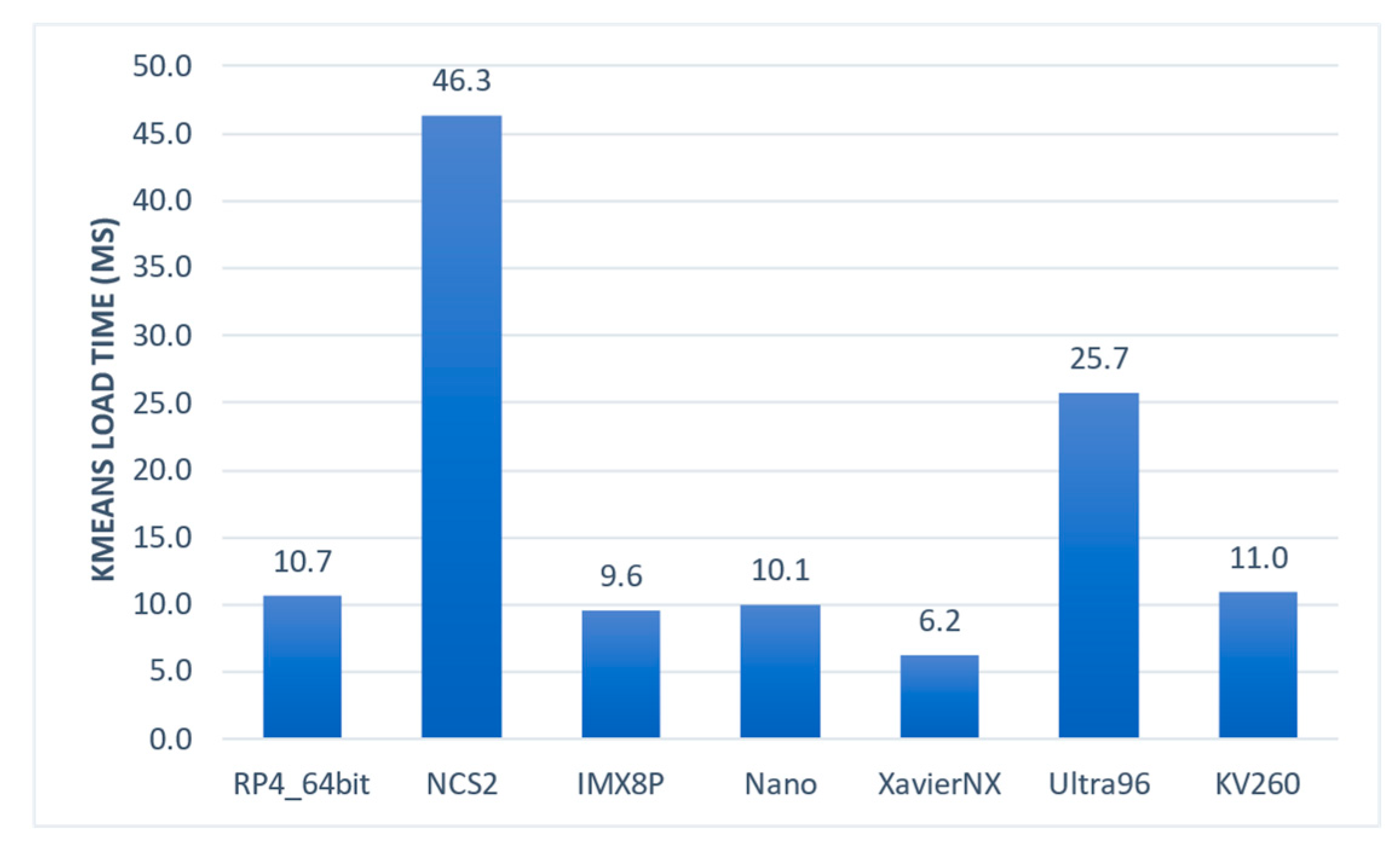
- Load k-means Model (Latency)
- 3.
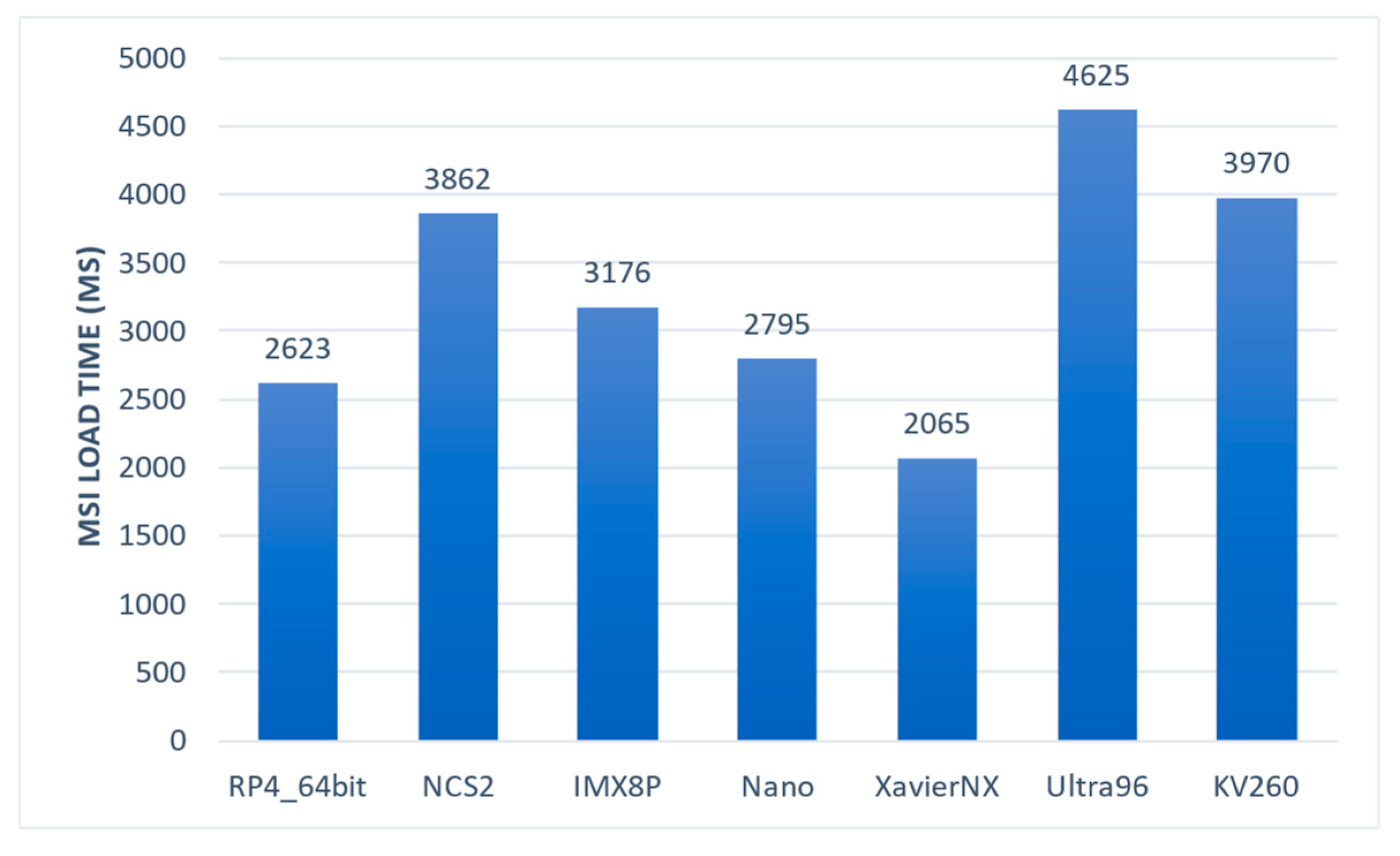
- Read MSI Samples (Latency)
- 4.
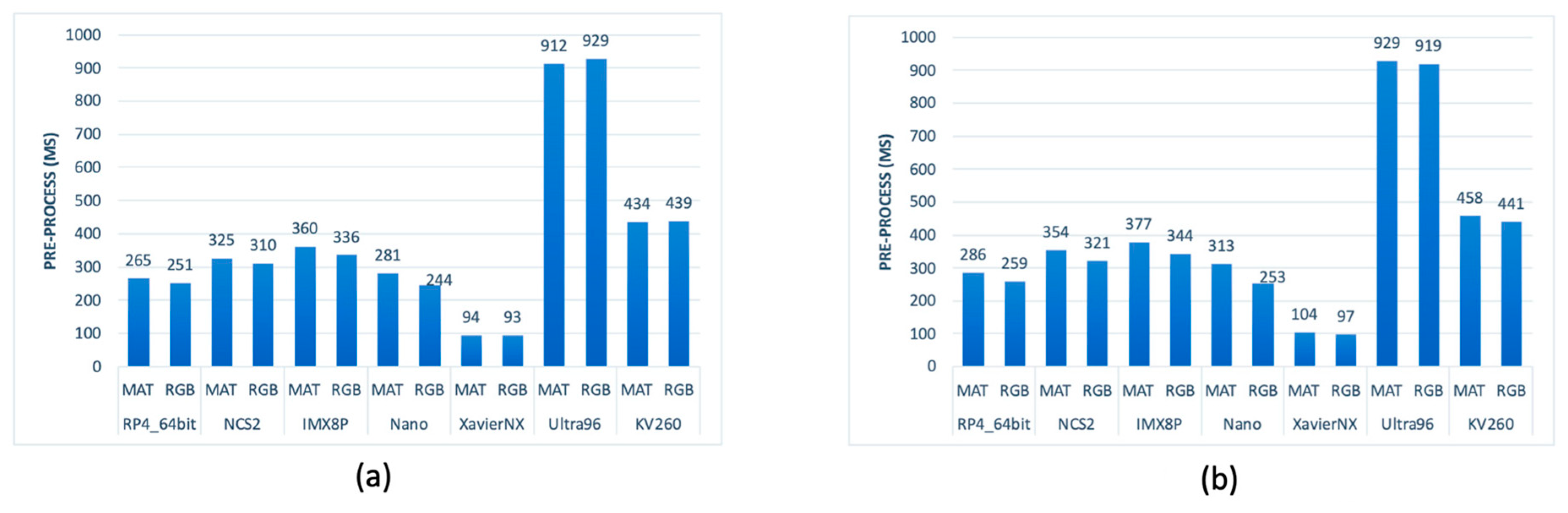
- Pre-Processing (Latency)
- 5.
- CNN Regression Model Inference Time (Latency)
- 6.
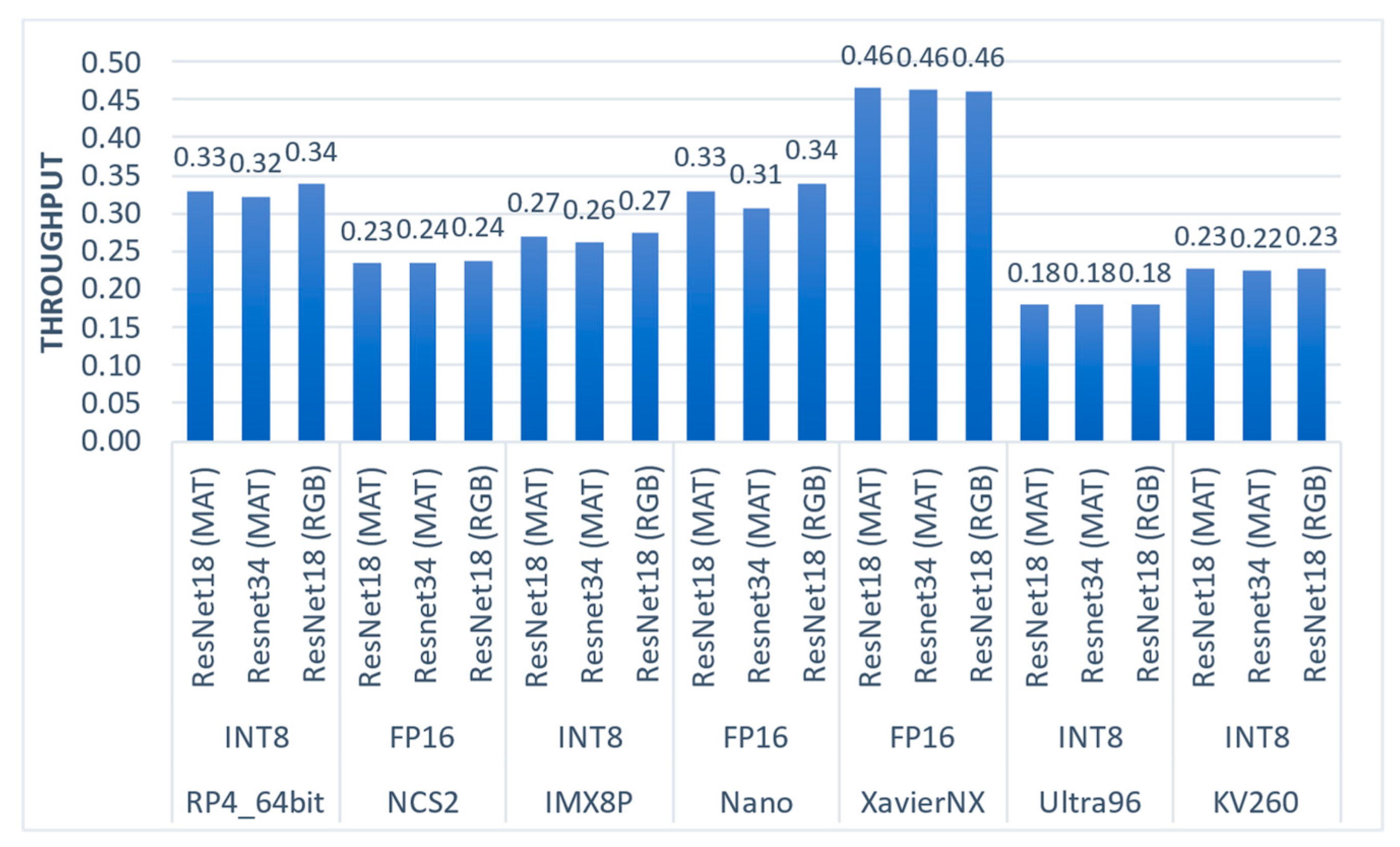
- Throughput (samples per second)
- 7.
- Efficiency (throughput per watt)
- 8.
- Value (throughput per dollar)
5. Conclusions
Author Contributions
Funding
Institutional Review Board Statement
Informed Consent Statement
Data Availability Statement
Conflicts of Interest
References
- Zhu, L.; Spachos, P.; Pensini, E.; Plataniotis, K.N. Deep learning and machine vision for food processing: A survey. Curr. Res. Food Sci. 2021, 4, 233–249. [Google Scholar] [CrossRef] [PubMed]
- Bodirsky, B.L.; Rolinski, S.; Biewald, A.; Weindl, I.; Popp, A.; Lotze-Campen, H. Global Food Demand Scenarios for the 21st Century. PLoS ONE 2015, 10, e0139201. [Google Scholar] [CrossRef] [PubMed]
- Fengou, L.-C.; Mporas, I.; Spyrelli, E.; Lianou, A.; Nychas, G.-J. Estimation of the Microbiological Quality of Meat Using Rapid and Non-Invasive Spectroscopic Sensors. IEEE Access 2020, 8, 106614–106628. [Google Scholar] [CrossRef]
- Nychas, G.-J.E.; Panagou, E.Z.; Mohareb, F. Novel approaches for food safety management and communication. Curr. Opin. Food Sci. 2016, 12, 13–20. [Google Scholar] [CrossRef]
- Bhunia, A.K. One day to one hour: How quickly can foodborne pathogens be detected? Future Microbiol. 2014, 9, 935–946. [Google Scholar] [CrossRef] [PubMed]
- Doulgeraki, A.I.; Nychas, G.-J.E. Monitoring the succession of the biota grown on a selective medium for pseudomonads during storage of minced beef with molecular-based methods. Food Microbiol. 2013, 34, 62–69. [Google Scholar] [CrossRef] [PubMed]
- Munir, M.T.; Yu, W.; Young, B.R.; Wilson, D.I. The current status of process analytical technologies in the dairy industry. Trends Food Sci. Technol. 2015, 43, 205–218. [Google Scholar] [CrossRef]
- van den Berg, F.; Lyndgaard, C.B.; Sørensen, K.M.; Engelsen, S.B. Process Analytical Technology in the food industry. Trends Food Sci. Technol. 2013, 31, 27–35. [Google Scholar] [CrossRef]
- Govari, M.; Tryfinopoulou, P.; Parlapani, F.F.; Boziaris, I.S.; Panagou, E.Z.; Nychas, G.-J.E. Quest of Intelligent Research Tools for Rapid Evaluation of Fish Quality: FTIR Spectroscopy and Multispectral Imaging Versus Microbiological Analysis. Foods 2021, 10, 264. [Google Scholar] [CrossRef]
- El Orche, A.; Mamad, A.; Elhamdaoui, O.; Cheikh, A.; El Karbane, M.; Bouatia, M. Comparison of Machine Learning Classification Methods for Determining the Geographical Origin of Raw Milk Using Vibrational Spectroscopy. J. Spectrosc. 2021, 2021, 5845422. [Google Scholar] [CrossRef]
- Ozturk, S.; Bowler, A.; Rady, A.; Watson, N.J. Near-infrared spectroscopy and machine learning for classification of food powders during a continuous process. J. Food Eng. 2023, 341, 111339. [Google Scholar] [CrossRef]
- Zhao, H.; Zhan, Y.; Xu, Z.; Nduwamungu, J.J.; Zhou, Y.; Powers, R.; Xu, C. The application of machine-learning and Raman spectroscopy for the rapid detection of edible oils type and adulteration. Food Chem. 2022, 373, 131471. [Google Scholar] [CrossRef] [PubMed]
- Nychas, G.-J.; Sims, E.; Tsakanikas, P.; Mohareb, F. Data Science in the Food Industry. Annu. Rev. Biomed. Data Sci. 2021, 4, 341–367. [Google Scholar] [CrossRef] [PubMed]
- Rodriguez-Saona, L.; Aykas, D.P.; Borba, K.R.; Urtubia, A. Miniaturization of optical sensors and their potential for high-throughput screening of foods. Curr. Opin. Food Sci. 2020, 31, 136–150. [Google Scholar] [CrossRef]
- McVey, C.; Elliott, C.T.; Cannavan, A.; Kelly, S.D.; Petchkongkaew, A.; Haughey, S.A. Portable spectroscopy for high throughput food authenticity screening: Advancements in technology and integration into digital traceability systems. Trends Food Sci. Technol. 2021, 118, 777–790. [Google Scholar] [CrossRef]
- Chen, X.; Cheng, G.; Liu, S.; Meng, S.; Jiao, Y.; Zhang, W.; Liang, J.; Zhang, W.; Wang, B.; Xu, X.; et al. Probing 1D convolutional neural network adapted to near-infrared spectroscopy for efficient classification of mixed fish. Spectrochim. Acta Part A Mol. Biomol. Spectrosc. 2022, 279, 121350. [Google Scholar] [CrossRef]
- Pu, H.; Yu, J.; Sun, D.-W.; Wei, Q.; Shen, X.; Wang, Z. Distinguishing fresh and frozen-thawed beef using hyperspectral imaging technology combined with convolutional neural networks. Microchem. J. 2023, 189, 108559. [Google Scholar] [CrossRef]
- Moon, E.J.; Kim, Y.; Xu, Y.; Na, Y.; Giaccia, A.J.; Lee, J.H. Evaluation of Salmon, Tuna, and Beef Freshness Using a Portable Spectrometer. Sensors 2020, 20, 4299. [Google Scholar] [CrossRef]
- Karunathilaka, S.R.; Yakes, B.J.; He, K.; Brückner, L.; Mossoba, M.M. First use of handheld Raman spectroscopic devices and on-board chemometric analysis for the detection of milk powder adulteration. Food Control. 2018, 92, 137–146. [Google Scholar] [CrossRef]
- Kolosov, D.; Mporas, I. Face Masks Usage Monitoring for Public Health Security using Computer Vision on Hardware. In Proceedings of the 2021 International Carnahan Conference on Security Technology (ICCST), Hatfield, UK, 11–15 October 2021; pp. 1–6. [Google Scholar] [CrossRef]
- Kolosov, D.; Kelefouras, V.; Kourtessis, P.; Mporas, I. Anatomy of Deep Learning Image Classification and Object Detection on Commercial Edge Devices: A Case Study on Face Mask Detection. IEEE Access 2022, 10, 109167–109186. [Google Scholar] [CrossRef]
- Carstensen, J.M.; Folm-Hansen, J. An Apparatus and a Method of Recording an Image of an Object. Google Patents WO1999042900, 26 August 1999. [Google Scholar]
- Sandler, M.; Howard, A.; Zhu, M.; Zhmoginov, A.; Chen, L.-C. MobileNetV2: Inverted Residuals and Linear Bottlenecks. In Proceedings of the 2018 IEEE/CVF Conference on Computer Vision and Pattern Recognition, Salt Lake City, UT, USA, 18–23 June 2018; pp. 4510–4520. [Google Scholar] [CrossRef]
- Huang, G.; Liu, Z.; Van Der Maaten, L.; Weinberger, K.Q. Densely Connected Convolutional Networks. In Proceedings of the 2017 IEEE Conference on Computer Vision and Pattern Recognition (CVPR), Honolulu, HI, USA, 21–26 July 2017; pp. 2261–2269. [Google Scholar] [CrossRef]
- Tan, M.; Le, Q.V. EfficientNet: Rethinking Model Scaling for Convolutional Neural Networks. In Proceedings of the International conference on Machine Learning (PMLR), Long Beach, CA, USA, 9–15 June 2019; pp. 6105–6114. [Google Scholar]
- Simonyan, K.; Zisserman, A. Very Deep Convolutional Networks for Large-Scale Image Recognition. In Proceedings of the International Conference on Learning Representations (ICLR), San Diego, CA, USA, 7–9 May 2015. [Google Scholar]
- He, K.; Zhang, X.; Ren, S.; Sun, J. Deep Residual Learning for Image Recognition. In Proceedings of the 2016 IEEE Conference on Computer Vision and Pattern Recognition (CVPR), Las Vegas, NV, USA, 27–30 June 2016; pp. 770–778. [Google Scholar] [CrossRef]
- Raspberry Pi 4 Model B Specifications. Available online: https://www.raspberrypi.org/products/raspberry-pi-4-model-b/ (accessed on 13 March 2023).
- Intel Neural Compute Stick 2 Product Specifications. Available online: https://ark.intel.com/content/www/us/en/ark/products/140109/intel-neural-compute-stick-2.html (accessed on 13 March 2023).
- Evaluation Kit for the i.MX 8M Plus Applications Processor. Available online: https://www.nxp.com/design/development-boards/i-mx-evaluation-and-development-boards/evaluation-kit-for-the-i-mx-8m-plus-applications-processor:8MPLUSLPD4-EVK (accessed on 13 March 2023).
- Jetson Nano Developer Kit. Available online: https://developer.nvidia.com/blog/jetson-nano-ai-computing/ (accessed on 13 March 2023).
- Jetson Xavier NX Series. Available online: https://www.nvidia.com/en-us/autonomous-machines/embedded-systems/jetson-xavier-nx/ (accessed on 13 March 2023).
- Ultra96. Available online: https://www.96boards.org/product/ultra96/ (accessed on 13 March 2023).
- Kria KV260 Vision AI Starter Kit. Available online: https://www.xilinx.com/products/som/kria/kv260-vision-starter-kit.html (accessed on 13 March 2023).
- Fengou, L.-C.; Lianou, A.; Tsakanikas, P.; Gkana, E.N.; Panagou, E.Z.; Nychas, G.-J.E. Evaluation of Fourier transform infrared spectroscopy and multispectral imaging as means of estimating the microbiological spoilage of farmed sea bream. Food Microbiol. 2019, 79, 27–34. [Google Scholar] [CrossRef] [PubMed]
- Tsakanikas, P.; Fengou, L.-C.; Manthou, E.; Lianou, A.; Panagou, E.Z.; Nychas, G.-J.E. A unified spectra analysis workflow for the assessment of microbial contamination of ready-to-eat green salads: Comparative study and application of non-invasive sensors. Comput. Electron. Agric. 2018, 155, 212–219. [Google Scholar] [CrossRef]
- Ropodi, A.I.; Panagou, E.Z.; Nychas, G.-J.E. Data mining derived from food analyses using non-invasive/non-destructive analytical techniques; determination of food authenticity, quality & safety in tandem with computer science disciplines. Trends Food Sci. Technol. 2016, 50, 11–25. [Google Scholar] [CrossRef]
- He, H.-J.; Sun, D.-W. Microbial evaluation of raw and processed food products by Visible/Infrared, Raman and Fluorescence spectroscopy. Trends Food Sci. Technol. 2015, 46, 199–210. [Google Scholar] [CrossRef]
- Zhao, H.-T.; Feng, Y.-Z.; Chen, W.; Jia, G.-F. Application of invasive weed optimization and least square support vector machine for prediction of beef adulteration with spoiled beef based on visible near-infrared (Vis-NIR) hyperspectral imaging. Meat Sci. 2019, 151, 75–81. [Google Scholar] [CrossRef]
- Cheng, J.-H.; Sun, D.-W. Rapid and non-invasive detection of fish microbial spoilage by visible and near infrared hyperspectral imaging and multivariate analysis. LWT-Food Sci. Technol. 2015, 62, 1060–1068. [Google Scholar] [CrossRef]
- Feng, C.-H.; Makino, Y.; Oshita, S.; Martín, J.F.G. Hyperspectral imaging and multispectral imaging as the novel techniques for detecting defects in raw and processed meat products: Current state-of-the-art research advances. Food Control 2018, 84, 165–176. [Google Scholar] [CrossRef]
- Yang, D.; Lu, A.; Ren, D.; Wang, J. Detection of total viable count in spiced beef using hyperspectral imaging combined with wavelet transform and multiway partial least squares algorithm. J. Food Saf. 2018, 38, e12390. [Google Scholar] [CrossRef]
- Baek, I.; Lee, H.; Cho, B.; Mo, C.; Chan, D.E.; Kim, M.S. Shortwave infrared hyperspectral imaging system coupled with multivariable method for TVB-N measurement in pork. Food Control 2021, 124, 107854. [Google Scholar] [CrossRef]
- Guo, T.; Huang, M.; Zhu, Q.; Guo, Y.; Qin, J. Hyperspectral image-based multi-feature integration for TVB-N measurement in pork. J. Food Eng. 2018, 218, 61–68. [Google Scholar] [CrossRef]
- Zhuang, Q.; Peng, Y.; Yang, D.; Nie, S.; Guo, Q.; Wang, Y.; Zhao, R. UV-fluorescence imaging for real-time non-destructive monitoring of pork freshness. Food Chem. 2022, 396, 133673. [Google Scholar] [CrossRef] [PubMed]


| Train Set (Number of Samples) | Train TVC Range log CFU/g | Test Set (Number of Samples) | Test TVC Range log CFU/g |
|---|---|---|---|
| R1, R2, R3 (312) | 3.08–10.32 | R4 (112) | 3.08–9.45 |
| R1, R2, R4 (312) | 2.00–9.93 | R3 (112) | 3.60–9.90 |
| R1, R3, R4 (324) | 2.00–10.32 | R2 (100) | 3.36–9.93 |
| R2, R3, R4 (324) | 2.00–10.32 | R1 (100) | 3.08–9.80 |
| Train Set (Number of Samples) | Train TVC Range log CFU/g | Test Set (Number of Samples) | Test TVC Range log CFU/g |
|---|---|---|---|
| R1, R2, R3 (308) | 3.76–9.45 | R4 (115) | 3.81–9.37 |
| R1, R2, R4 (307) | 2.30–9.37 | R3 (116) | 3.76–9.22 |
| R1, R3, R4 (323) | 2.30–9.45 | R2 (100) | 4.60–8.90 |
| R2, R3, R4 (331) | 2.30–9.45 | R1 (92) | 4.70–8.70 |
| Layer Name | Output Size | ResNet-18 | ResNet-34 |
|---|---|---|---|
| input | - | ||
| conv_1x | |||
| conv_2x | |||
| conv_3x | |||
| conv_4x | |||
| conv_5x | |||
| output | average pool, linear | ||
| # | Hardware | CPU | Memory | AI Accelerator | AI Runtime Engine |
|---|---|---|---|---|---|
| 1 | RP4_64bit [28] | ARM Cortex-A72 | 8 GB (LPDDR4) | N/A * | TFLITE |
| 2 | RP4_32bit [28] | ARM Cortex-A72 | 4 GB (LPDDR4) | N/A * | OpenVINO |
| NCS2 [29] | N/A | 500 MB (Internal) | VPU | ||
| 3 | IMX8P [30] | ARM Cortex-A53 | 4 GB (LPDDR4) | NPU | TFLITE |
| 4 | Nano [31] | ARM Cortex-A57 | 4 GB (LPDDR4) | GPU: 128-core Maxwell | TensorRT |
| 5 | XavierNX [32] | Carmel ARM®v8.2 | 8 GB (LPDDR4) | GPU: 384-core Volta | TensorRT |
| 6 | Ultra96 [33] | ARM Cortex-A53 | 2 GB (LPDDR4) | PL: DPU (B1600) | VART |
| 7 | KV260 [34] | ARM Cortex-A53 | 4 GB (LPDDR4) | PL: DPU (B4096) | VART |
| Model | Parameters | Type | Masking | r | RMSE | MAE | RPD |
|---|---|---|---|---|---|---|---|
| ResNet-18 | 11,186,625 | RGB | NO | 0.86 | 0.07 | 0.08 | 1.71 |
| ResNet-18 | 11,233,665 | MSI | NO | 0.95 | 0.07 | 0.05 | 2.83 |
| ResNet-34 | 21,349,249 | MSI | NO | 0.95 | 0.07 | 0.05 | 2.72 |
| ResNet-18 | 11,186,625 | RGB | YES | 0.86 | 0.11 | 0.08 | 1.76 |
| ResNet-18 | 11,233,665 | MSI | YES | 0.94 | 0.07 | 0.05 | 2.90 |
| ResNet-34 | 21,349,249 | MSI | YES | 0.95 | 0.09 | 0.05 | 2.68 |
| Model | Parameters | Type | Masking | r | RMSE | MAE | RPD |
|---|---|---|---|---|---|---|---|
| ResNet-18 | 11,186,625 | RGB | NO | 0.80 | 0.09 | 0.07 | 1.37 |
| ResNet-18 | 11,233,665 | MSI | NO | 0.90 | 0.06 | 0.05 | 1.81 |
| ResNet-34 | 21,349,249 | MSI | NO | 0.89 | 0.07 | 0.05 | 1.84 |
| ResNet-18 | 11,186,625 | RGB | YES | 0.76 | 0.08 | 0.07 | 1.29 |
| ResNet-18 | 11,233,665 | MSI | YES | 0.89 | 0.09 | 0.05 | 1.88 |
| ResNet-34 | 21,349,249 | MSI | YES | 0.89 | 0.11 | 0.06 | 1.68 |
| Type | Data Type | r | RMSE | MAE | RPD |
|---|---|---|---|---|---|
| TF | FP32 (original) | 0.89 | 0.08 | 0.06 | 2.04 |
| TFLITE | FP16 | 0.00 | 0.00 | 0.00 | 0.00 |
| TFLITE | DINT8 | 0.00 | 0.00 | 0.00 | 0.01 |
| TFLITE | PTQ-INT8 * | 0.03 | −0.03 | −0.03 | 0.35 |
| OpenVINO | FP16 | 0.00 | 0.00 | 0.00 | 0.04 |
| TRT | FP16 | 0.00 | 0.00 | 0.00 | 0.00 |
| TRT | PTQ-INT8 | 0.27 | −0.07 | −0.06 | 1.33 |
| VITIS | PTQ-INT8 | 0.02 | −0.02 | −0.02 | 0.30 |
| VART | PTQ-INT8 | 0.01 | −0.02 | −0.02 | 0.25 |
| Platform | Data Type | Model | Type | Inference Time (ms) | |||
|---|---|---|---|---|---|---|---|
| 1× | 2× | 3× | 4× | ||||
| RP4_64bit * | INT8 | ResNet-18 | MSI | 316.6 | 189.0 | 144.0 | 125.9 |
| ResNet-34 | MSI | 530.3 | 312.3 | 231.9 | 200.0 | ||
| ResNet-18 | RGB | 238.2 | 140.7 | 105.6 | 92.8 | ||
| NCS2 | FP16 | ResNet-18 | MSI | 61.7 | - | - | - |
| ResNet-34 | MSI | 79.2 | - | - | - | ||
| ResNet-18 | RGB | 24.5 | - | - | - | ||
| IMX8P * | INT8 | ResNet-18 | MSI | 534.7 | 293.7 | 212.8 | 174.8 |
| ResNet-34 | MSI | 913.5 | 493.6 | 352.7 | 281.7 | ||
| ResNet-18 | RGB | 404.9 | 221.9 | 160.2 | 129.3 | ||
| Nano | FP16 | ResNet-18 | MSI | 18.3 | - | - | - |
| ResNet-34 | MSI | 26.9 | - | - | - | ||
| ResNet-18 | RGB | 12.1 | - | - | - | ||
| XavierNX | FP16 | ResNet-18 | MSI | 4.3 | - | - | - |
| ResNet-34 | MSI | 5.9 | - | - | - | ||
| ResNet-18 | RGB | 3.0 | - | - | - | ||
| Ultra96 | INT8 | ResNet-18 | MSI | 39.0 | - | - | - |
| ResNet-34 | MSI | 52.7 | - | - | - | ||
| ResNet-18 | RGB | 20.6 | - | - | - | ||
| KV260 | INT8 | ResNet-18 | MSI | 19.7 | - | - | - |
| ResNet-34 | MSI | 22.8 | - | - | - | ||
| ResNet-18 | RGB | 6.9 | - | - | - | ||
Disclaimer/Publisher’s Note: The statements, opinions and data contained in all publications are solely those of the individual author(s) and contributor(s) and not of MDPI and/or the editor(s). MDPI and/or the editor(s) disclaim responsibility for any injury to people or property resulting from any ideas, methods, instructions or products referred to in the content. |
© 2023 by the authors. Licensee MDPI, Basel, Switzerland. This article is an open access article distributed under the terms and conditions of the Creative Commons Attribution (CC BY) license (https://creativecommons.org/licenses/by/4.0/).
Share and Cite
Kolosov, D.; Fengou, L.-C.; Carstensen, J.M.; Schultz, N.; Nychas, G.-J.; Mporas, I. Microbiological Quality Estimation of Meat Using Deep CNNs on Embedded Hardware Systems. Sensors 2023, 23, 4233. https://doi.org/10.3390/s23094233
Kolosov D, Fengou L-C, Carstensen JM, Schultz N, Nychas G-J, Mporas I. Microbiological Quality Estimation of Meat Using Deep CNNs on Embedded Hardware Systems. Sensors. 2023; 23(9):4233. https://doi.org/10.3390/s23094233
Chicago/Turabian StyleKolosov, Dimitrios, Lemonia-Christina Fengou, Jens Michael Carstensen, Nette Schultz, George-John Nychas, and Iosif Mporas. 2023. "Microbiological Quality Estimation of Meat Using Deep CNNs on Embedded Hardware Systems" Sensors 23, no. 9: 4233. https://doi.org/10.3390/s23094233