
Towards Real-Time Analysis of Gas-Liquid Pipe Flow: A Wire-Mesh Sensor for Industrial Applications
 , , and
Abstract
:1. Introduction
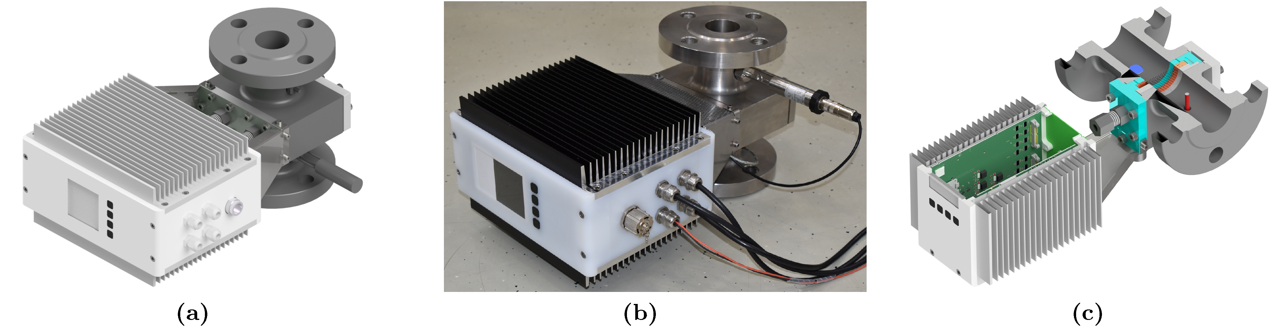
2. Design of an Industrial Wire-Mesh Sensor
2.1. Design of a Robust Sensor Body
2.2. Electronics Design
2.3. Data Processing
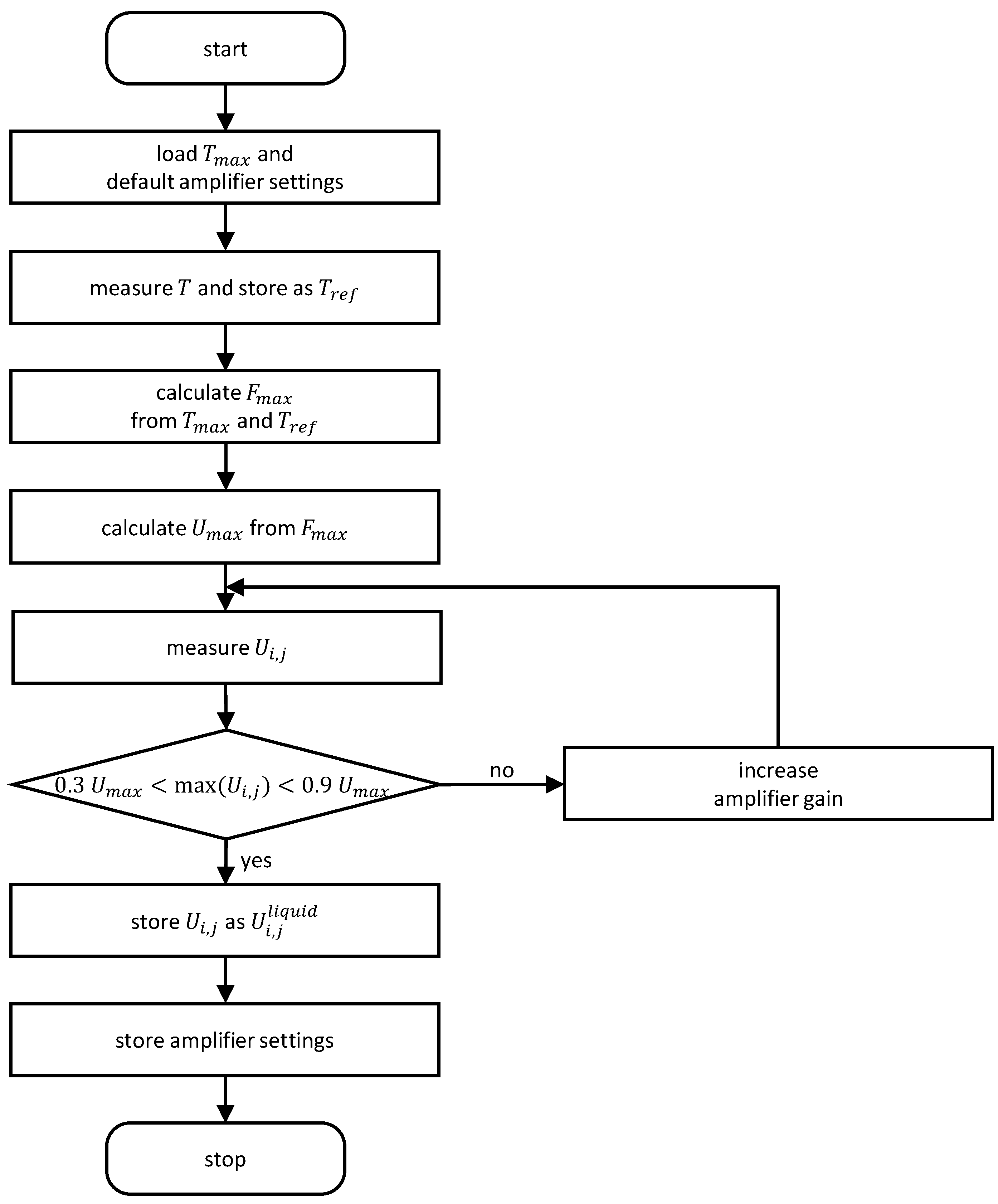
2.3.1. Temperature Compensation and Calculation of Cross-Sectionally Averaged Phase Fraction
2.3.2. Flow Pattern Identification
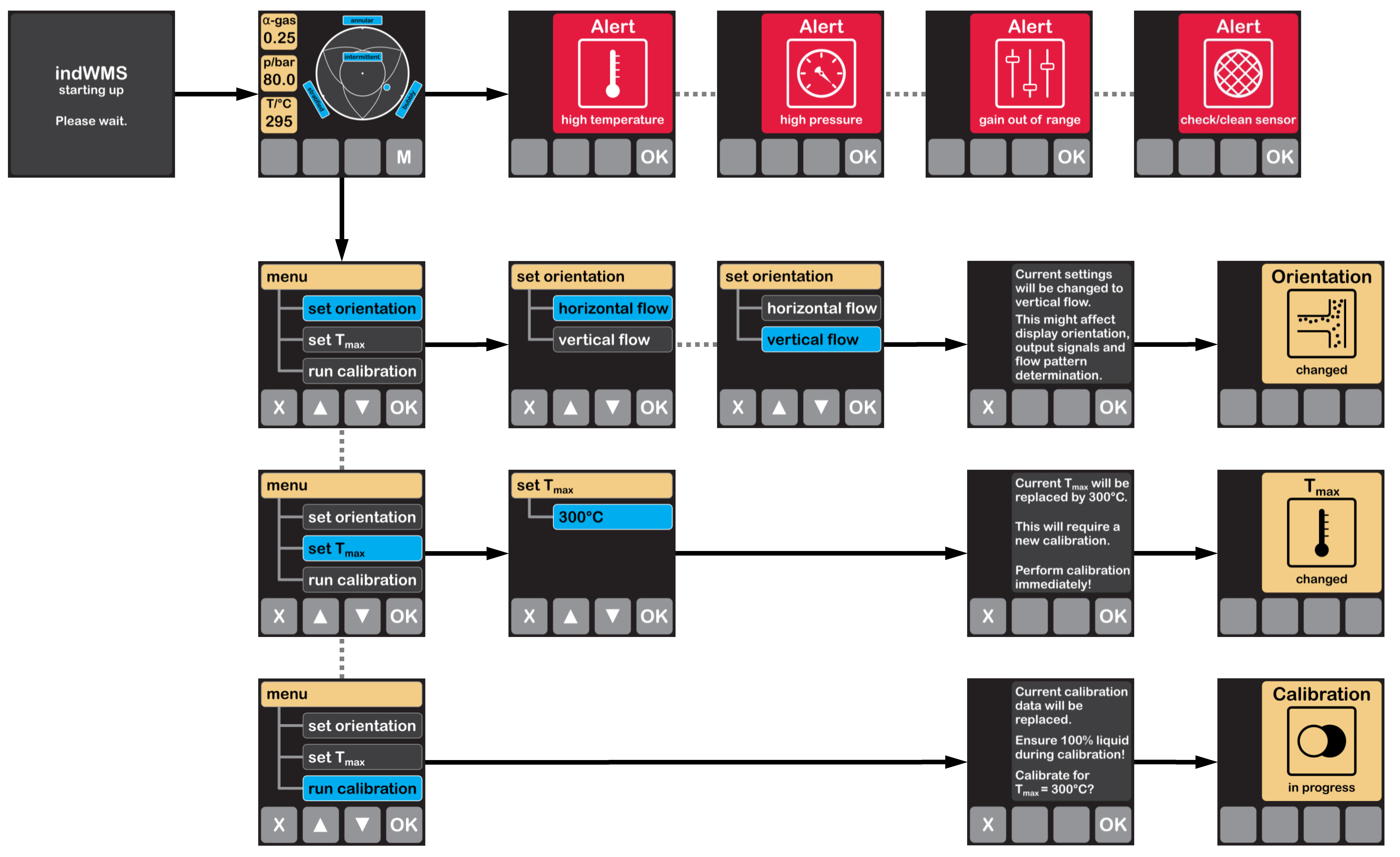
2.4. User Interface
- Switching between horizontal and vertical orientations leads to activation of the respective flow pattern identification algorithm and its visualization scheme on the main screen as well as to a change in the display orientation.
- Adjusting the expected maximum temperature of the two-phase flow is required for the calibration routine, which is explained below.
- Running the calibration routine.
3. Experimental Verification
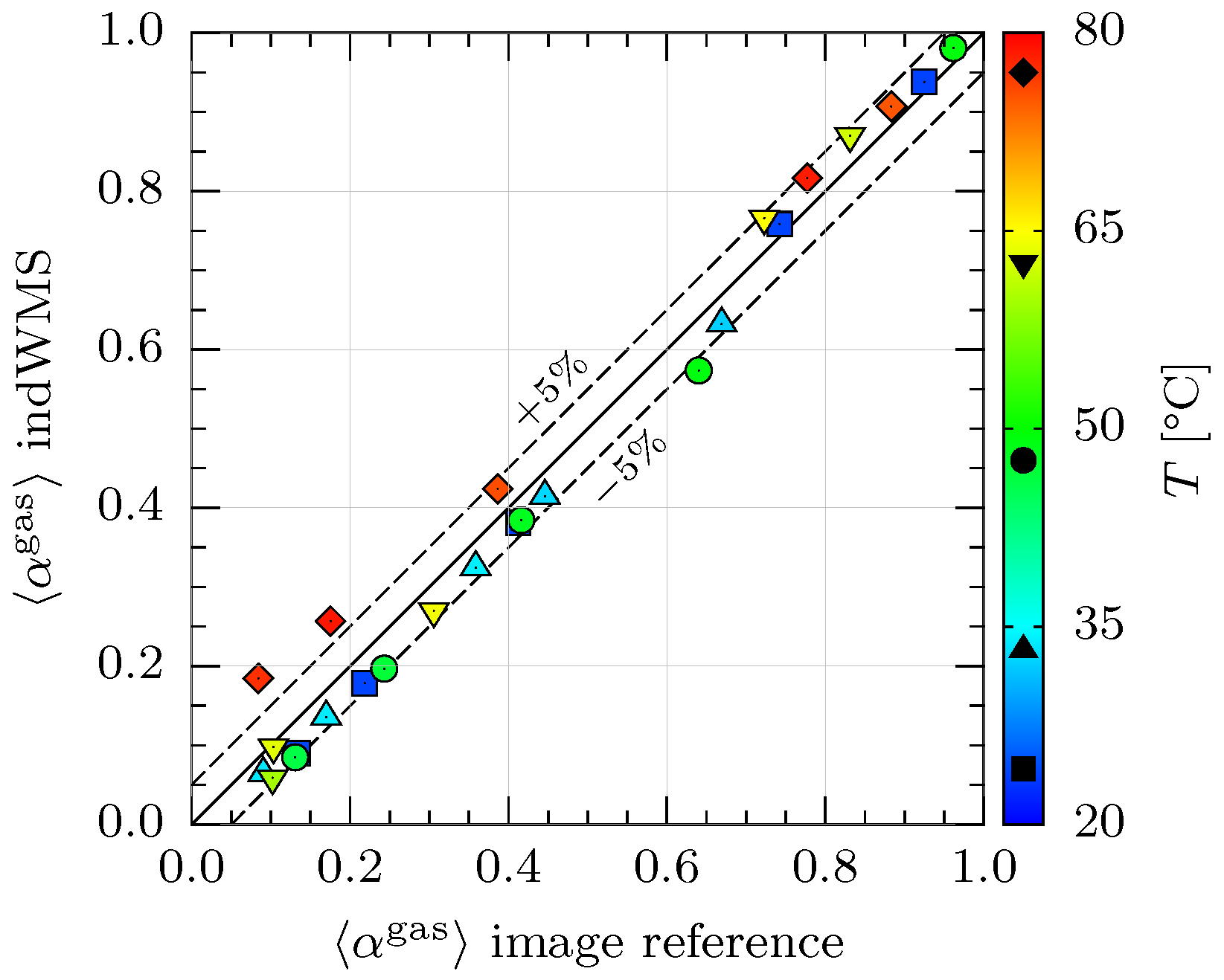
3.1. Temperature Compensation
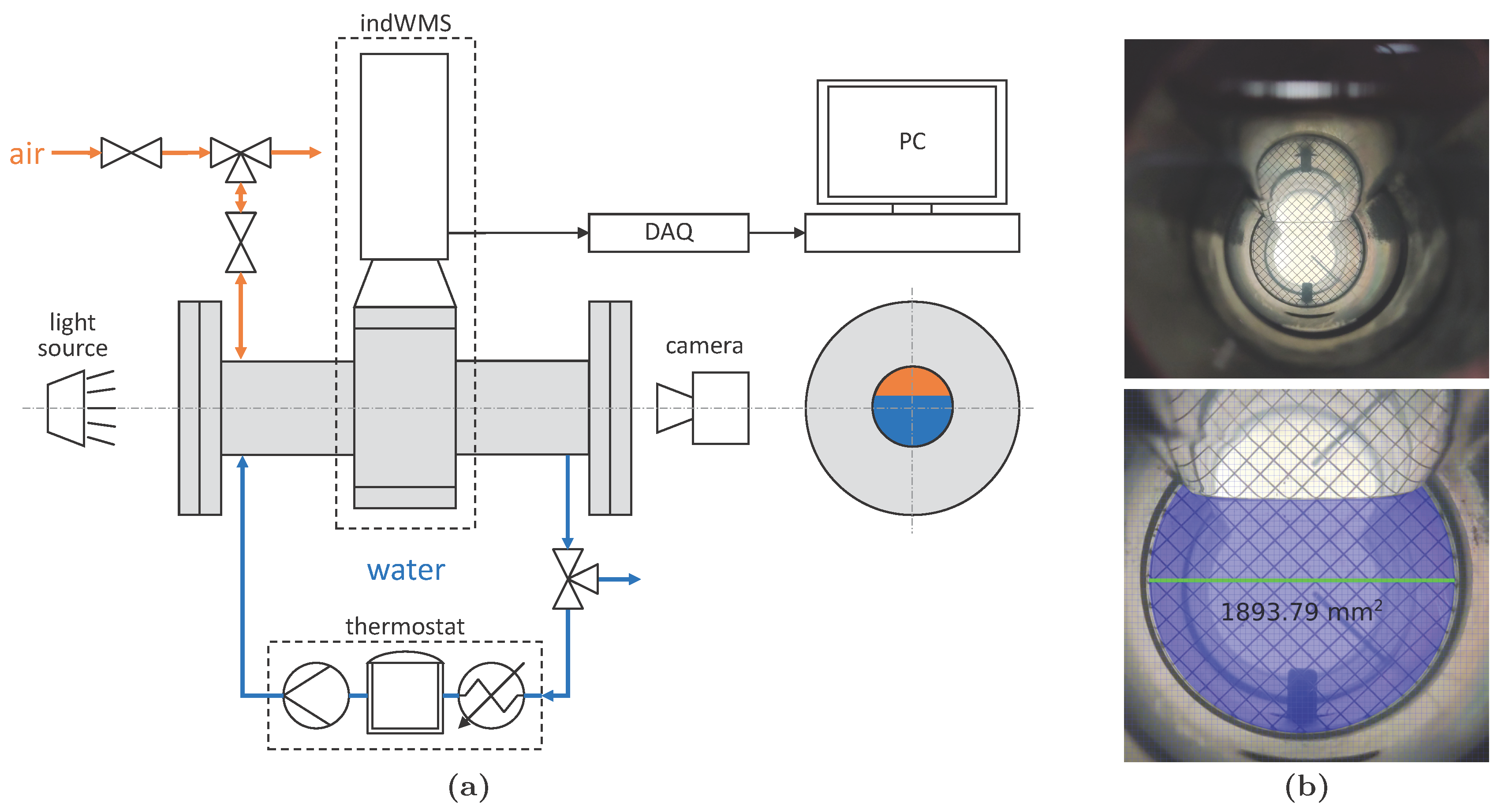
3.1.1. Experimental Procedure
- Image cropping;
- Image scaling according to the pipe’s inner diameter (green line in Figure 5b);
- Approximating the gas–liquid interface in the stratified state within a concentric circle of the pipe’s inner diameter (taking menisci at the pipe wall into consideration);
- Calculating the area or of the remaining geometry (blue area in Figure 5b).
3.1.2. Results and Discussion
3.2. Real-Time Flow Pattern Identification
3.2.1. Experimental Procedure
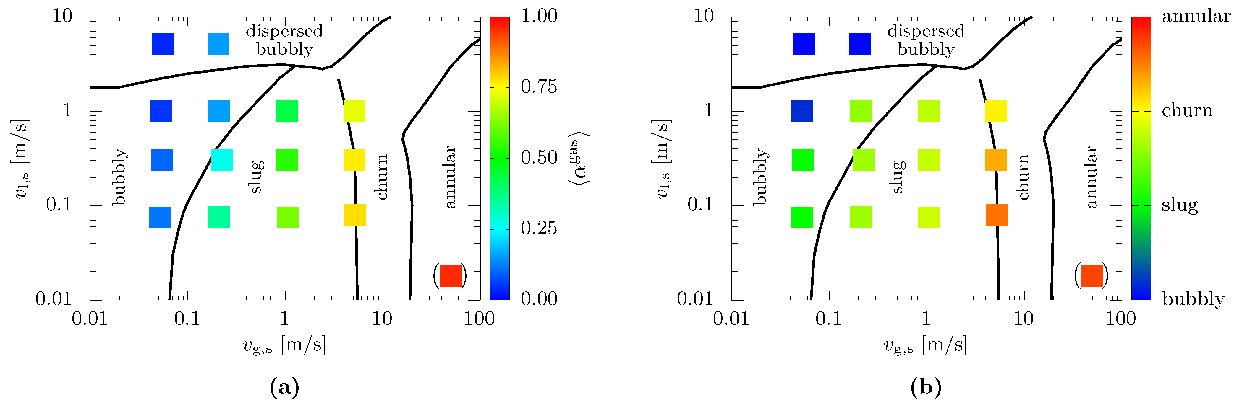
3.2.2. Results of Cross-Sectional Phase Fraction and Flow Pattern Identification in Vertical Pipes
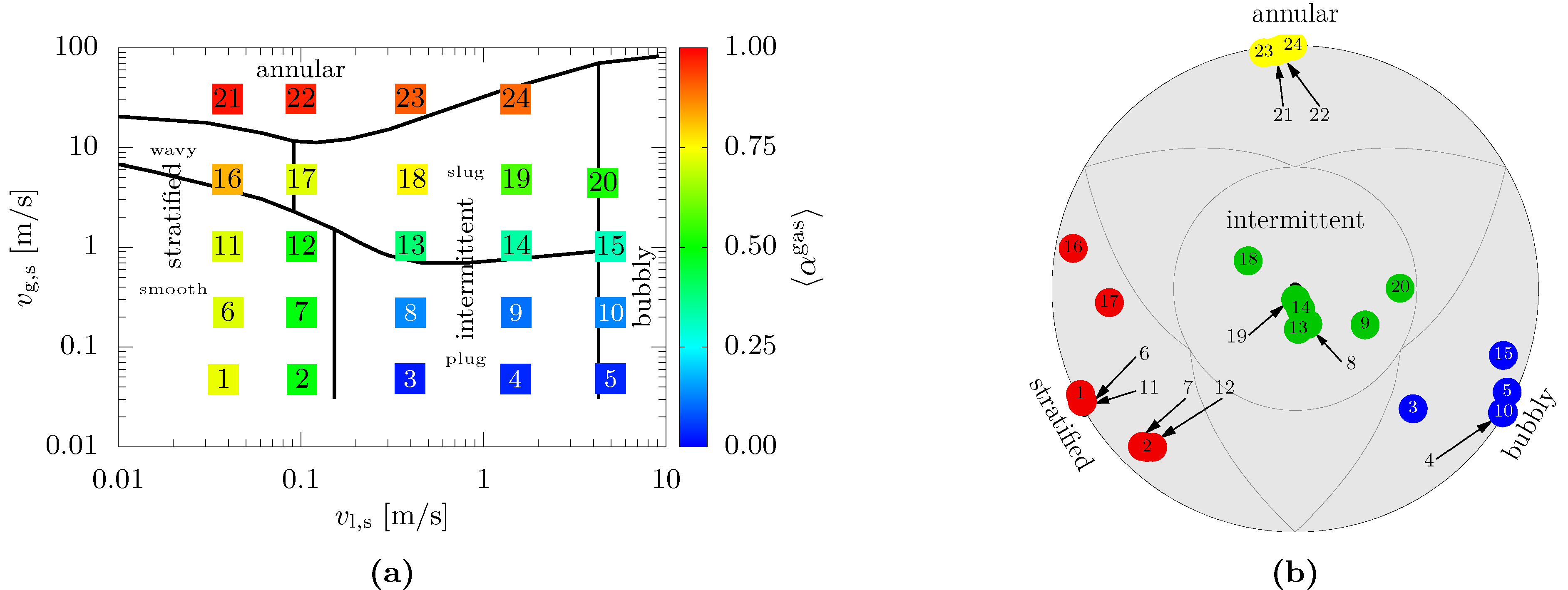
3.2.3. Results of Cross-Sectional Phase Fraction and Flow Pattern Identification in Horizontal Pipes
4. Conclusions
Author Contributions
Funding
Data Availability Statement
Acknowledgments
Conflicts of Interest
References
- Hansen, L.S.; Pedersen, S.; Durdevic, P. Multi-Phase Flow Metering in Offshore Oil and Gas Transportation Pipelines: Trends and Perspectives. Sensors 2019, 19, 2184. [Google Scholar] [CrossRef]
- Hampel, U.; Babout, L.; Banasiak, R.; Schleicher, E.; Soleimani, M.; Wondrak, T.; Vauhkonen, M.; Lähivaara, T.; Tan, C.; Hoyle, B.; et al. A Review on Fast Tomographic Imaging Techniques and Their Potential Application in Industrial Process Control. Sensors 2022, 22, 2309. [Google Scholar] [CrossRef] [PubMed]
- Prasser, H.-M.; Böttger, A.; Zschau, J. A new electrode-mesh tomograph for gas-liquid flows. Flow Meas. Instrum. 1998, 9, 111–119. [Google Scholar] [CrossRef]
- Wangjiraniran, W.; Motegi, Y.; Richter, S.; Kikura, M.; Aritomi, M.; Yamamoto, K. Intrusive Effect of Wire Mesh Tomography on Gas-liquid Flow Measurement. J. Nucl. Sci. Technol. 2003, 40, 932–940. [Google Scholar] [CrossRef]
- Ito, D.; Prasser, H.-M.; Kikura, H.; Aritomi, M. Uncertainty and intrusiveness of three-layer wire-mesh sensor. Flow Meas. Instrum. 2011, 22, 249–256. [Google Scholar] [CrossRef]
- Tompkins, C.; Prasser, H.-M.; Corradini, M. Wire-mesh sensors: A review of methods and uncertainty in multiphase flows relative to other measurement techniques. Nucl. Eng. Des. 2018, 337, 205–220. [Google Scholar] [CrossRef]
- Dias, F.D.A.; Ripa, D.R.; Morales, R.E.M.; da Silva, M.J. Wire-Mesh Sensor Super-Resolution Based on Statistical Reconstruction. IEEE Trans. Instrum. Meas. 2021, 70, 4503212. [Google Scholar] [CrossRef]
- Prasser, H.-M.; Grunwald, G.; Höhne, T.; Kliem, S.; Rohde, U.; Weiss, F.-P. Coolant Mixing in a Pressurized Water Reactor: Deboration Transients, Steam-Line Breaks, and Emergency Core Cooling Injection. Nucl. Technol. 2017, 143, 37–56. [Google Scholar] [CrossRef]
- Parsi, M.; Vieira, R.E.; Torres, C.F.; Kesana, N.R.; McLaury, B.S.; Shirazi, S.A.; Schleicher, E.; Hampel, U. On the effect of liquid viscosity on interfacial structures within churn flow: Experimental study using wire mesh sensor. Chem. Eng. Sci. 2015, 130, 221–238. [Google Scholar] [CrossRef]
- Kesana, N.R.; Parsi, M.; Vieira, R.E.; Azzopardi, B.; Schleicher, E.; McLaury, B.S.; Shirazi, S.A.; Hampel, U. Visualization of gas-liquid multiphase pseudo-slug flow using Wire-Mesh Sensor. J. Nat. Gas Sci. Eng. 2017, 46, 477–490. [Google Scholar] [CrossRef]
- Timaeus, R.; Berger, R.; Schleicher, E.; Hampel, U.; Schubert, M. Liquid Flow Visualization in Packed-Bed Multiphase Reactors: Wire-Mesh Sensor Design and Data Analysis for Rotating Fixed Beds. Chem. Ing. Tech. 2019, 91, 1812–1821. [Google Scholar] [CrossRef]
- Brinkmann, J.H.; Plate, D.; Merkel, A.; Seithümmer, V.B.; Biessey, P.; Grünewald, M. Application of a wire-mesh sensor for the experimental characterization of liquid distribution in packed columns. Chem. Eng. Sci. 2021, 242, 116721. [Google Scholar] [CrossRef]
- Vishwakarma, V.; Schleicher, E.; Bieberle, A.; Schubert, M.; Hampel, U. Advanced flow profiler for two-phase flow imaging on distillation trays. Chem. Eng. Sci. 2021, 231, 116280. [Google Scholar] [CrossRef]
- Hoffmann, A.; Schleicher, E.; Keller, L.; León Alonso, J.; Pitz-Paal, R. Application of a single wire-mesh sensor in a parabolic trough facility with direct steam generation. Sol. Energy 2018, 159, 1016–1030. [Google Scholar] [CrossRef]
- Kipping, R.; Brito, R.; Schleicher, E.; Hampel, U. Developments for the application of the Wire-Mesh Sensor in industries. Int. J. Multiph. Flow 2016, 85, 86–95. [Google Scholar] [CrossRef]
- Schleicher, E.; Tschofen, M.; Pietruske, H. Gittersensor-System Zum Charakterisieren Einer Fluidströmung. German Patent DE102015117084B3, 19 May 2016. [Google Scholar]
- Pietruske, H.; Prasser, H.-M. Wire-mesh sensors for high-resolving two-phase flow studies at high pressures and temperatures. Flow Meas. Instrum. 2007, 18, 87–94. [Google Scholar] [CrossRef]
- Pietruske, H.; Sühnel, T.; Prasser, H.-M. Gittersensor. German Patent DE102005019739B3, 26 October 2006. [Google Scholar]
- da Silva, M.J.; Schleicher, E.; Hampel, U. Capacitance wire-mesh sensor for fast measurement of phase fraction distributions. Meas. Sci. Technol. 2007, 18, 2245–2251. [Google Scholar] [CrossRef]
- dos Santos, E.N.; Vendruscolo, T.P.; Morales, R.E.M.; Schleicher, E.; Hampel, U.; Da Silva, M.J. Dual-modality wire-mesh sensor for the visualization of three-phase flows. Meas. Sci. Technol. 2015, 26, 105302. [Google Scholar] [CrossRef]
- Dias, F.D.A.; dos Santos, E.N.; da Silva, M.J.; Schleicher, E.; Morales, R.E.; Hewakandamby, B.; Hampel, U. New Algorithm to Discriminate Phase Distribution of Gas-Oil-Water Pipe Flow with Dual-Modality Wire-Mesh Sensor. IEEE Access 2020, 8, 125163–125178. [Google Scholar] [CrossRef]
- Wiedemann, P.; de Assis Dias, F.; Schleicher, E.; Hampel, U. Temperature Compensation for Conductivity-Based Phase Fraction Measurements with Wire-Mesh Sensors in Gas-Liquid Flows of Dilute Aqueous Solutions. Sensors 2020, 20, 7114. [Google Scholar] [CrossRef]
- Deutsches Institut für Normung. Water Quality—Determination of Electrical Conductivity, German Version EN 27888: 1993. ISO 7888: 1985; Beuth Verlag: Berlin, Germany, 1993. [Google Scholar]
- Wiedemann, P.; Döß, A.; Schleicher, E.; Hampel, U. Fuzzy flow pattern identification in horizontal air-water two-phase flow based on wire-mesh sensor data. Int. J. Multiph. Flow 2019, 117, 153–162. [Google Scholar] [CrossRef]
- Drahoš, J.; Čermák, J. Diagnostics of gas-liquid flow patterns in chemical engineeing systems. Chem. Eng. Process. 1989, 26, 147–164. [Google Scholar] [CrossRef]
- Barnea, D. A unified model for predicting flow-pattern transitions for the whole range of pipe inclinations. Int. J. Multiph. Flow 1987, 13, 1–12. [Google Scholar] [CrossRef]
- Jones, O.C., Jr.; Zuber, N. The interrelation between void fraction fluctuations and flow patterns in two-phase flow. Int. J. Multiph. Flow 1975, 2, 273–306. [Google Scholar] [CrossRef]
- Rosa, E.S.; Salgado, R.M.; Ohishi, T.; Mastelari, N. Performance comparison of artificial neural networks and expert systems applied to flow pattern identification in vertical ascendant gas-liquid flows. Int. J. Multiph. Flow 2010, 36, 738–754. [Google Scholar] [CrossRef]
- Mandhane, J.M.; Gregory, G.A.; Aziz, K. A flow pattern map for gas-liquid flow in horizontal pipes. Int. J. Multiph. Flow 1974, 1, 537–553. [Google Scholar] [CrossRef]
- Abbagoni, B.M.; Yeung, H. Non-invasive classification of gas-liquid two-phase horizontal flow regimes using an ultrasonic doppler sensor and a neural network. Meas. Sci. Technol. 2016, 27, 084002. [Google Scholar] [CrossRef]
- Roman, A.J.; Kreitzer, P.J.; Ervin, J.S.; Hanchak, M.S.; Byrd, L.W. Flow pattern identification of horizontal two-phase refrigerant flow using neural networks. Int. Commun. Heat Mass Transf. 2016, 71, 254–264. [Google Scholar] [CrossRef]
- Sun, Z.; Chen, Y.; Gong, H. Classification of gas-liquid flow patterns by the norm entropy of wavelet decomposed pressure fluctuations across a bluff body. Meas. Sci. Technol. 2012, 23, 125301. [Google Scholar] [CrossRef]


Disclaimer/Publisher’s Note: The statements, opinions and data contained in all publications are solely those of the individual author(s) and contributor(s) and not of MDPI and/or the editor(s). MDPI and/or the editor(s) disclaim responsibility for any injury to people or property resulting from any ideas, methods, instructions or products referred to in the content. |
© 2023 by the authors. Licensee MDPI, Basel, Switzerland. This article is an open access article distributed under the terms and conditions of the Creative Commons Attribution (CC BY) license (https://creativecommons.org/licenses/by/4.0/).
Share and Cite
Wiedemann, P.; de Assis Dias, F.; Trepte, M.; Schleicher, E.; Hampel, U. Towards Real-Time Analysis of Gas-Liquid Pipe Flow: A Wire-Mesh Sensor for Industrial Applications. Sensors 2023, 23, 4067. https://doi.org/10.3390/s23084067
Wiedemann P, de Assis Dias F, Trepte M, Schleicher E, Hampel U. Towards Real-Time Analysis of Gas-Liquid Pipe Flow: A Wire-Mesh Sensor for Industrial Applications. Sensors. 2023; 23(8):4067. https://doi.org/10.3390/s23084067
Chicago/Turabian StyleWiedemann, Philipp, Felipe de Assis Dias, Manuel Trepte, Eckhard Schleicher, and Uwe Hampel. 2023. "Towards Real-Time Analysis of Gas-Liquid Pipe Flow: A Wire-Mesh Sensor for Industrial Applications" Sensors 23, no. 8: 4067. https://doi.org/10.3390/s23084067