
An Improvement Strategy for Indoor Air Quality Monitoring Systems †

Abstract
:1. Introduction
2. Methods and Applications
2.1. Monitored Parameter
2.2. IAQ Index Calculation
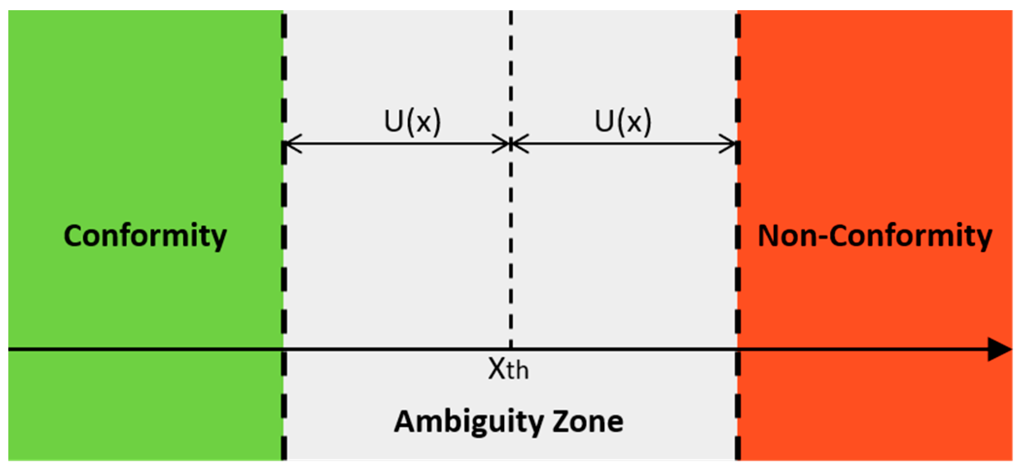
3. Data Uncertainty and Decision Making
3.1. Data Uncertainty and Decision-Making Problems
3.2. Decision-Making Algorithms
3.2.1. Utility Cost Test
- u++ when the value is below the threshold and is correctly classified as such;
- u+− when the value is below the threshold and is incorrectly classified above
- the threshold;
- u−+ when the value is above the threshold and is incorrectly classified below
- the threshold;
- u−− when the value is above the threshold and is correctly classified as such,
- with u++ > u+− e u−− > u−+.
3.2.2. Fixed Risk
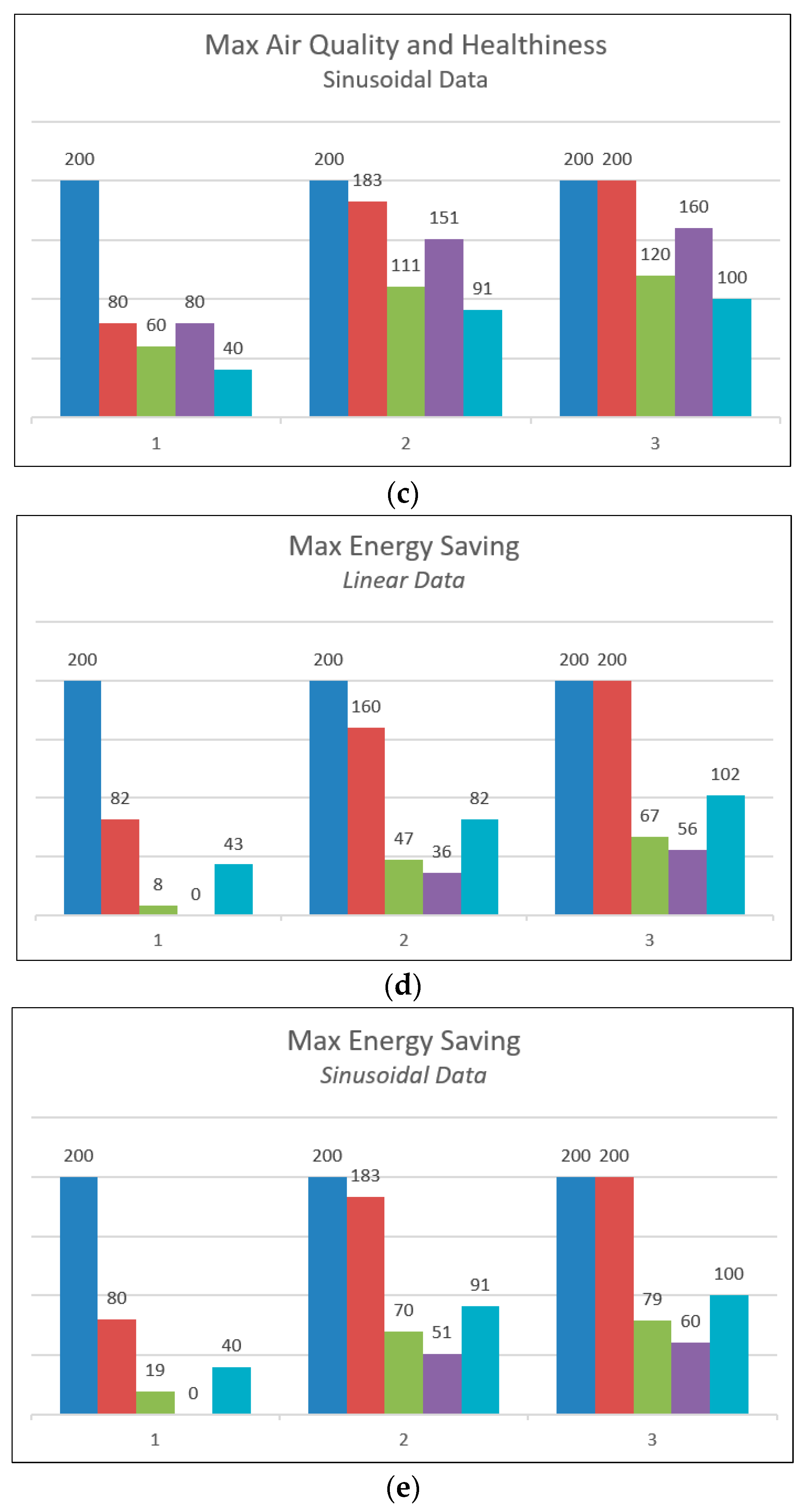
3.3. Validation of Decision-Making Algorithms
- Max Air Quality and Healthiness
- Max Energy Saving
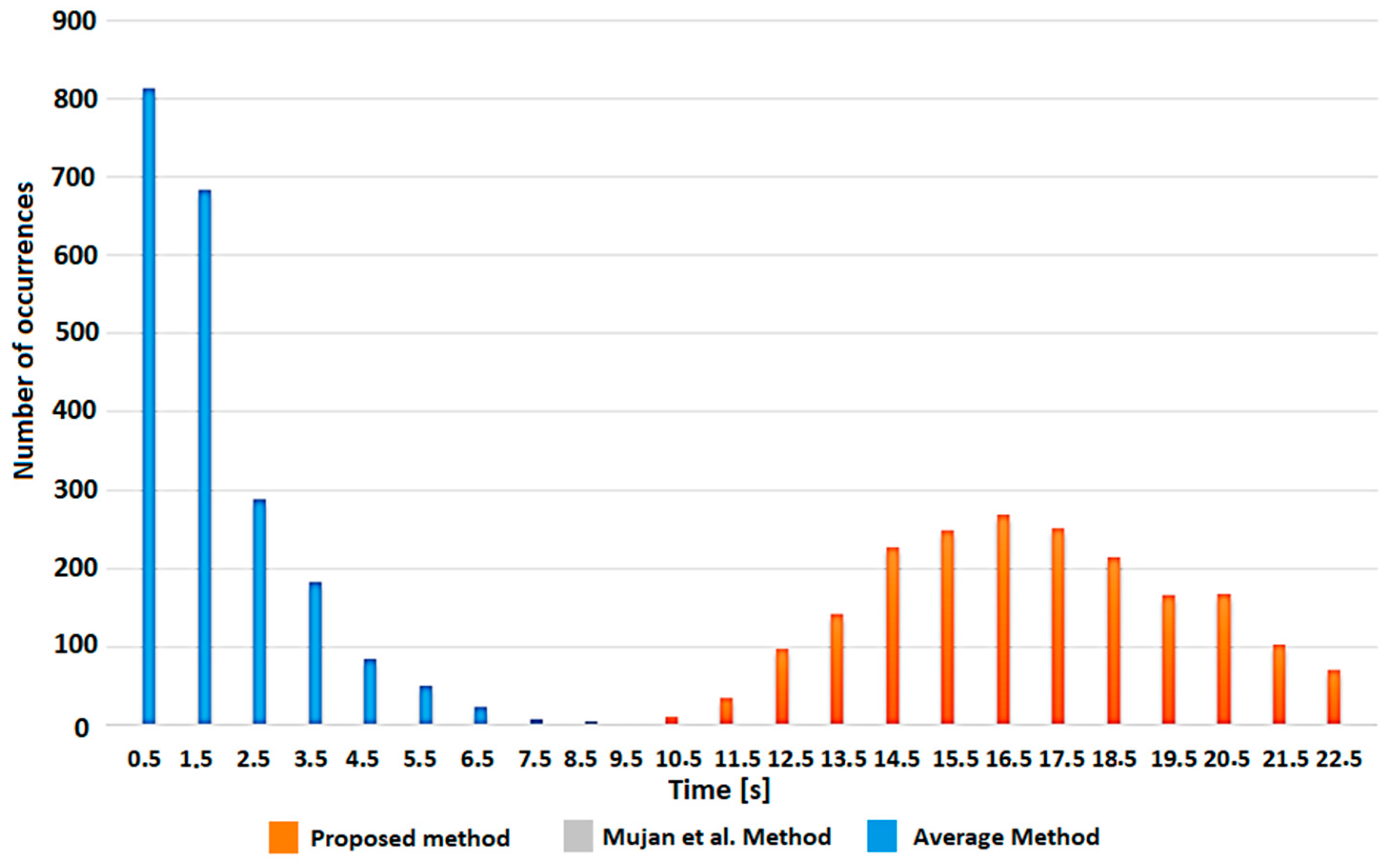
4. Results
5. Conclusions and Future Perspectives
Author Contributions
Funding
Institutional Review Board Statement
Informed Consent Statement
Data Availability Statement
Conflicts of Interest
Appendix A
| Listing A1. Pseudo-code of the control station algorithm |
| define COthreshold, CO2threshold,VOCthreshold,PMthreshold; define COuncertainty, CO2uncertainty, VOCuncertainty, PMuncertainty; define alfa0CO, alfa1CO, alfa2CO, alfa0CO2, alfa1CO2, alfa2CO2, alfa0VOC, alfa1VOC, alfa2VOC, alfa0PM, alfa1PM, alfa2PM; define optimalCO, optimalCO2, optimalVOC, optimalPM; define comfortThreshold; define acquisitionRate; setup(){ \* select strategy and set activateVentilation to FALSE (ventilation OFF) strategy=keyboard.in(); decisionMakingType=keyboard.in(); startTime=getTime(); activateVentilation=FALSE; } main(){ while(STOP){ previoustime = time; COreading[] = CO.insert(sensorRead(sensor1)); CO2reading[] = CO2.insert(sensorRead(sensor2)); VOCreading[] = VOC.insert(sensorRead(sensor3)); PMreading[] = PM.insert(sensorRead(sensor4)); outdoorCOreading[] = outdoorCOreading.insert(sensorRead(sensor5)); outdoorCO2reading[] = outdoorCO2reading.insert (sensorRead(sensor6)); outdoorVOCreading[] = outdoorVOCreading.insert(sensorRead(sensor7)); outdoorPMreading[] = outdoorPMreading.insert(sensorRead(sensor8)); time = getTime(); maxdimension 900/acquisitionRate; /* number of samples in 15m if(outdoorCOreading.size()>maxdimension){ COreading.delete(0); CO2reading.delete(0); VOCreading.delete(0); PMreading.delete(0); outdoorCOreading.delete(0); outdoorCO2reading.delete(0); outdoorVOCreading.delete(0); outdoorPMreading.delete(0); } \*Calculate cumulative values of pollutants during monitoring interval cumulativeCO=cumulativeCO+TrapezoidalRuleIntegral(COreading.lastElement(), COreading.lastElement()-1, time, previousTime); cumulativeCO2=cumulativeCO2+TrapezoidalRuleIntegral(CO2reading.lastElement(), CO2reading.lastElement()-1, time, previousTime); cumulativeVOC=cumulativeVOC+TrapezoidalRuleIntegral(VOCreading.lastElement(), VOCreading.lastElement()-1, time, previousTime); cumulativePM=cumulativePM+TrapezoidalRuleIntegral(PMreading.lastElement(), PMreading.lastElement()-1, time, previousTime); \*Calculate the optimal cumulative value of pollutants (ideal case) cumulativeOptimalCO=cumulativeOptimalCO+TrapezoidalRuleIntegral(optimalCO, optimalCO, time, previousTime); cumulativeOptimalCO2=cumulativeOptimalCO2+TrapezoidalRuleIntegral(optimalCO2, optimalCO2, time, previousTime); cumulativeOptimalVOC=cumulativeOptimalVOC+TrapezoidalRuleIntegral(optimalVOC, optimalVOC, time, previousTime); cumulativeOptimalPM=cumulativeOptimalPM+TrapezoidalRuleIntegral(optimalPM, optimalPM, time, previousTime); \* if values in ambiguity zone call DecisionMaking subroutine to assign a value to activateVentilation if(COreading.lastElement()>=COthreshold-COuncertainty && COreading.lastElement()<=COthreshold+COuncertainty){ activateVentilation=DecisionMaking(strategy, decisionMakingType, COreading.lastElement(), COuncertainty, COthreshold);} else if(CO2reading.lastElement()>=CO2threshold-CO2uncertainty && CO2reading.lastElement()<=CO2threshold+CO2uncertainty){ activateVentilation=DecisionMaking(strategy, decisionMakingType, CO2reading.lastElement(), CO2uncertainty, CO2threshold);} else if(VOCreading.lastElement()>=VOCthreshold-VOCuncertainty && VOCreading.lastElement()<=VOCthreshold+VOCuncertainty){ activateVentilation=DecisionMaking(strategy, decisionMakingType, VOCreading.lastElement(), VOCuncertainty, VOCthreshold);} else if(PMreading.lastElement()>=PMthreshold-PMuncertainty && PMreading.lastElement()<=PMthreshold+PMuncertainty){ activateVentilation=DecisionMaking(strategy, decisionMakingType, PMreading.lastElement(), PMuncertainty, PMthreshold);} \* if not in ambiguity zone verify if one or more pollutant levels are above safety thresholds and if it is the case activate ventilation. else if (COreading.lastElement()>COthreshold+COuncertainty || CO2reading.lastElement()>CO2threshold+CO2uncertainty ||VOCreading.lastElement()>VOCthreshold+VOCuncertainty || PMreading.lastElement()>PMthreshold+PMuncertainty){ activateVentilation=TRUE; } else{ \* calculate cumulative indices as in Equation (3) and IAQ index as in equation 5, if IAQ level is below comfortThreshold, calculate relative indices as in equation 6, referring to the last 15 min, and relative IAQ as in Equation (7). If relative IAQ is less than zero activate ventilation. alfaCOt = alfa0CO + alfa1CO*time+ alfa2CO*time^2; ICO = 100 − alfaCOt*log(cumulativeCO/cumulativeOptimalCO); alfaCO2t = alfa0CO2 + alfa1CO2*time + alfa2CO2*time^2; ICO2 = 100 − alfaCO2t*log(cumulativeCO2/cumulativeOptimalCO2); alfaVOCt = alfa0VOC + alfa1VOC*time + alfa2VOC*time^2; IVOC = 100-alfaVOCt*log(cumulativeVOC/cumulativeOptimalVOC); alfaPMt = alfa0PM + alfa1PM*time alfa2PM*time^2; IPM = 100-alfaPMt*log(cumulativePM/cumulativeOptimalPM); IAQ = min(ICO, ICO2, IVOC, IPM); if(IAQ < comfortThreshold){ ICOrelative = 100-alfaCOt*log(Integral(COreading, time, time-900)/Integral(outdoorCOreading, time, time-900)); ICO2relative = 100-alfaCO2t*log(Integral(CO2reading, time, time-900)/Integral(outdoorCO2reading, time, time-900)); IVOCrelative = 100-alfaVOCt*log(Integral(VOCreading, time, time-900)/Integral(outdoorVOCreading, time, time-900)); IPMrelative = 100-alfaPMt*log(Integral(PMreading, time, time-900)/Integral(outdoorPMreading, time, time-900)); relativeIAQ = min(ICOrelative, ICO2relative, IVOCrelative, IPMrelative); if(relativeIAQ < 0){ activateVentilation = TRUE; } } } if(activateVentilation==TRUE){ VentilationON(); wait(900s); VentilationOFF(); activateVentilation=FALSE; resetAllVariables(); } } } subroutine boolean DecisionMaking(strategy, decisionMakingType, measurementData, uncertainty, threshold){ \*chose between the two algorithms and call the specific subroutine if(decisionMakingType==“UtilityCostTest”){ return UtilityCostTest(strategy, measurementData, uncertainty, threshold);} else return FixedRisk(strategy, measurementData, uncertainty, threshold); } |
| Listing A2. Pseudo-code of Utility Cost Test algorithm |
| subroutine boolean UtilityCostTest (strategy, measurementData, uncertainty, threshold){ u[] = UtilitySetParameters(strategy); pdf[] = ProbabilityDensityFunction(measurementData, uncertainty) pA = Integral(pdf,threshold,-infty); p0 = (u[3] − u[2])/(u[0] − u[1] − u[2] + u[3]) if(pA > p0) return FALSE; else return TRUE; } |
| Listing A3. Pseudo-code of Fixed Risk algorithm |
| subroutine boolean FixedRisk (strategy, measurementData, uncertainty, threshold){ mra=FixedSetParameters(strategy); pdf[]=ProbabilityDensityFunction(measurementData, uncertainty) cumulativePdf[]= Integral(pdf); xmra=cumulativePdf.getIndexAtElement(mra); if(measurementData>xmra) return TRUE; else return FALSE; } |
References
- Palco, V.; Fulco, G.; De Capua CRuffa, F.; Lugara, M. IoT and IAQ monitoring systems for healthiness of dwelling. In Proceedings of the 2022 IEEE International Workshop on Metrology for Living Environment, MetroLivEn 2022—Proceedings, Cosenza, Italy, 25–27 May 2022; pp. 105–109. [Google Scholar] [CrossRef]
- Fulco, G.; Ruffa, F.; Lugarà, M.; Filianoti, P.; De Capua, C. Automatic station for monitoring a microgrid. In Proceedings of the 24th IMEKO TC4 International Symposium and 22nd International Workshop on ADC and DAC Modelling and Testing, Palermo, Italy, 14–16 September 2022; pp. 309–314. [Google Scholar]
- Kwok, A.G.; Rajkovich, N.B. Addressing climate change in comfort standards. Build. Environ. 2010, 45, 18–22. [Google Scholar] [CrossRef]
- De Capua, A. La qualità ambientale indoor nella riqualificazione edilizia. In Legislazione Tecnica 1 Edizione; Legislazione Tecnica: Roma, Italy, October 2019; ISBN 978-88-6219-319-1. [Google Scholar]
- Fulco, G.; Palco, V. Sensoring e Iot: Abitare Smart. In Design in the Digital Age. Technology, Nature, Culture; Maggioli Editore: Emilia-Romagna, Italy, 2022; ISBN 978-88-916-4327-8. [Google Scholar]
- Yousef, A.H.; Arif, M.; Katafygiotou, M.; Mazroei, A.; Kaushik, A.; Elsarrag, E. Impact of indoor environmental quality on occupant well-being and comfort: A review of the literature. Int. J. Sustain. Built Environ. 2016, 5, 1–11. [Google Scholar] [CrossRef]
- Morawska, L.; Tang, J.W.; Bahnfleth, W.; Bluyssen, P.M.; Boerstra, A.; Buonanno, G.; Cao, J.; Dancer, S.; Floto, A.; Franchimon, F.; et al. How can airborne transmission of COVID-19 indoors be minimised? Environ. Int. 2020, 142, 105832. [Google Scholar] [CrossRef]
- Ashton, K. That ‘Internet of things’ Thing: In the Real World Things Matter More than Ideas. RFID Journal. Available online: http://www.rfidjournal.com/articles/view?4986 (accessed on 25 February 2020).
- Morello, R.; De Capua, C.; Lugarà, M. The Design of a Sensor Network Based on IoT Technology for Landslide Hazard Assessment. In Proceedings of the 4th Imeko TC19 Symposium on Environmental Instrumentation and Measurements Protecting Environment, Climate Changes and Pollution Control, Lecce, Italy, 3–4 June 2013; Volume 1, pp. 99–103. [Google Scholar]
- Daponte, P.; De Capua, C.; Liccardo, A. A technique for remote management of instrumentation based on Web Service. In Proceedings of the 13th IMEKO TC4 Symposium on Measurements for Research and Industrial Applications 2004, Held Together with the 9th Workshop on ADC Modeling and Testing, Athens, Greece, 29 September–1 October 2004; pp. 657–662. [Google Scholar]
- Catalina, T.; Iordache, V. IEQ assessment on schools in the design stage. Build. Environ. 2012, 49, 129–140. [Google Scholar] [CrossRef]
- Abdul-Wahab, S.A. Sick Building Syndrome in Public Buildings and Workplaces; Springer: Berlin/Heidelberg, Germany, 2011. [Google Scholar] [CrossRef]
- Olli, A.; Seppänen, W. Some Quantitative Relations between Indoor Environmental Quality and Work Performance or Health. ASHRAE Res. J. 2006, 12, 957–973. [Google Scholar] [CrossRef] [Green Version]
- Ahlawat, A.; Wiedensohler, A.; Mishra, S. An Overview on the Role of Relative Humidity in Airborne Transmission of SARS-CoV-2 in Indoor Environments. Aerosol Air Qual. Res. 2020, 20, 1856–1861. [Google Scholar] [CrossRef]
- Chan, K.H.; Malik Peiris, J.S.; Lam, S.Y.; Poon, L.M.; Yuen, K.Y.; Seto, W.H. The effects of temperature and relative humidity on the viability of the SARS coronavirus. Adv. Virol. 2011, 2011, 734690. [Google Scholar] [CrossRef] [PubMed]
- Wolkoff, P. Indoor air humidity, air quality, and health—An overview. Int. J. Hyg. Environ. Health 2018, 221, 376–390. [Google Scholar] [CrossRef] [PubMed]
- Serroni, S.; Arnesano, M.; Violini, L.; Revel, G.M. An IoT measurement solution for continuous indoor environmental quality monitoring for buildings renovation. Acta Imeko 2021, 10, 230–238. [Google Scholar] [CrossRef]
- Argunhan, Z.; Serkan Avci, A. Statistical Evaluation of Indoor Air Quality Parameters in Classrooms of a University. Adv. Meteorol. 2018, 2018, 4391579. [Google Scholar] [CrossRef]
- Fang, B.; Xu, Q.; Park, T.; Zhang, M. AirSense: An intelligent home-based sensing system for indoor air quality analytics. In Proceedings of the 2016 ACM International Joint Conference on Pervasive and Ubiquitous Computing Association for Computing Machinery, New York, NY, USA, 12–16 September 2016. [Google Scholar]
- Konstantinou, C.; Constantinou, V.; Kleovoulou, E.G.; Kyriacou, A.; Kakoulli, C.; Milis, G.; Michaelides, M.; Makris, K.C. Assessment of indoor and outdoor air quality in primary schools of Cyprus during the COVID–19 pandemic measures in May–July 2021. Heliyon 2022, 8, e09354. [Google Scholar] [CrossRef] [PubMed]
- Song, Y.; Mao, F.; Liu, Q. Human Comfort in Indoor Environment: A Review on Assessment Criteria, Data Collection and Data Analysis Methods. IEEE Access 2019, 7, 119774–119786. [Google Scholar] [CrossRef]
- Rodrigues dos Santos, R.; Gregório, J.; Castanheira, L.; Fernandes, A.S. Exploring Volatile Organic Compound Exposure and Its Association with Wheezing in Children under 36 Months: A Cross-Sectional Study in South Lisbon, Portugal. Int. J. Environ. Res. Public Health 2020, 17, 6929. [Google Scholar] [CrossRef]
- Lay-Ekuakille, A.; Vergallo, P.; Morello, R.; De Capua, C. Indoor air pollution system based on LED technology. Measurement 2014, 47, 749–755. [Google Scholar] [CrossRef]
- Lay-Ekuakille, A.; Ikezawa, S.; Mugnaini, M.; Morello, R.; De Capua, C. Detection of specific macro and micropollutants in air monitoring: Review of methods and techniques. Measurement 2017, 98, 49–59. [Google Scholar] [CrossRef]
- Chiesa, G.; Cesari, S.; Garcia, M.; Issa, M.; Li, S. Multisensor IoT Platform for Optimising IAQ Levels in Buildings through a Smart Ventilation System. Sustainability 2019, 11, 5777. [Google Scholar] [CrossRef] [Green Version]
- ISO 17772-1:2017; Energy Performance of Buildings. Indoor Environmental Quality. Indoor Environmental Input Parameters for the Design and Assessment of Energy Performance of Buildings. International Organization for Standardization (ISO): Geneva, Switzerland, 2017.
- Küçükhüseyin, Ö. CO2 monitoring and indoor air quality. REHVA Eur. HVAC J. 2021, 58, 55–59. [Google Scholar]
- Shin, M.S.; Rhee, K.N.; Lee, E.T.; Jung, G.J. Performance evaluation of CO2-based ventilation control to reduce CO2 concentration and condensation risk in residential buildings. Build. Environ. 2018, 142, 451–463. [Google Scholar] [CrossRef]
- Habeebullah, T.M.; Abd El-Rahim, I.H.; Morsy, E.A. Impact of outdoor and indoor meteorological conditions on the COVID-19 transmission in the western region of Saudi Arabia. J. Environ. Manag. 2021, 288, 112392. [Google Scholar] [CrossRef]
- Doremalen, N.; Bushmaker, T.; Morris, D.H.; Holbrook, M.G.; Gamble, A.; Williamson, B.N. Aerosol and surface stability of SARS-CoV-2 as compared with SARS-CoV-1. N. Engl. J. Med. 2020, 382, 1564–1567. [Google Scholar] [CrossRef]
- Khan, A.U.; Khan, M.E.; Hasan, M.; Zakri, W.; Alhazmi, W.; Islam, T. An Efficient Wireless Sensor Network Based on the ESP-MESH Protocol for Indoor and Outdoor Air Quality Monitoring. Sustainability 2022, 14, 16630. [Google Scholar] [CrossRef]
- Schiewecka, A.; Uhdea, E.; Salthammera, T.; Salthammerb, L.; Morawskac, L.; Mazaheric, M.; Kumard, P. Smart homes and the control of indoor air quality. Renew. Sustain. Energy Rev. 2018, 94, 705–718. [Google Scholar] [CrossRef]
- Costanzo, V.; Yao, R.; Xu, T.; Xiong, J.; Zhang, Q.; Li, B. Natural ventilation potential for residential buildings in a densely built-up and highly polluted environment. A case study. Renew. Energy 2019, 138, 340–353. [Google Scholar] [CrossRef]
- Mujan, I.; Licina, D.; Kljajic, M.; Culic, A.; Anđelkovic, A.S. Development of indoor environmental quality index using a low-cost monitoring platform. J. Clean. Prod. 2021, 312, 127846. [Google Scholar] [CrossRef]
- Abdul-Wahab, S.; Chin Fah En, S.; Elkamel, A.; Ahmadi, L.; Yetilmezsoy, K. A review os standard and guidelines set by international bodies for the parameters of indoor air quality. Atmos. Pollut. Res. 2015, 6, 751–767. [Google Scholar] [CrossRef]
- Baudet, A.; Baurès, E.; Blanchard, O.; Le Cann, P.; Gangneux, J.; Florentin, A. Indoor Carbon Dioxide, Fine Particulate Matter and Total Volatile Organic Compounds in Private Healthcare and Elderly Care Facilities. Toxics 2022, 10, 136. [Google Scholar] [CrossRef]
- Hapsari, A.A.; Hajamydeen, A.I.; Vresdian, D.J.; Manfaluthy, M.; Prameswono, L.; Yusuf, E. Real Time Indoor Air Quality Monitoring System Based on IoT using MQTT and Wireless Sensor Network. In Proceedings of the IEEE 6th International Conference on Engineering Technologies and Applied Sciences (ICETAS), Kuala Lumpur, Malaysia, 20–21 December 2019; pp. 1–7. [Google Scholar] [CrossRef]
- Pietrogrande, M.C.; Casari, L.; Demaria, G.; Russo, M. Indoor Air Quality in Domestic Environments during Periods Close to Italian COVID-19 Lockdown. Int. J. Environ. Res. Public Health 2021, 18, 4060. [Google Scholar] [CrossRef]
- Moreno-Rangel, A.; Sharpe, T.; Musau, F.; Mcgill, G. Field evaluation of a low-cost indoor air quality monitor to quantify exposure to pollutants in residential environments. J. Sens. Sens. Syst. 2018, 7, 373–388. [Google Scholar] [CrossRef] [Green Version]
- Shrestha, B.; Tiwari, S.; Bajracharya, S.; Keitsch, M. Role of gender participation in urban household energy technology for sustainability: A case of Kathmandu. Discov. Sustain. 2021, 2, 19. [Google Scholar] [CrossRef]
- Fernández-Agüera, J.; Dominguez-Amarillo, S.; Fornaciari, M.; Orlandi, F. TVOCs and PM 2.5 in Naturally Ventilated Homes: Three Case Studies in a Mild Climate. Sustainability 2019, 11, 6225. [Google Scholar] [CrossRef] [Green Version]
- Pongboonkhumlarp, N.; Jinsart, W. Health risk analysis from volatile organic compounds and fine particulate matter in the printing industry. Int. J. Environ. Sci. Technol. 2021, 19, 8633–8644. [Google Scholar] [CrossRef] [PubMed]
- Residential Indoor Air Quality Guidelines: Carbon Dioxide; Health Canada: Ottawa, ON, Canada, 2021; ISBN 978-0-660-37419-2.
- Zoran, M.A.; Savastru, R.S.; Savastru, D.M.; Tautan, M.N. Assessing the relationship between surface levels of PM2.5 and PM10 particulate matter impact on COVID-19 in Milan, Italy. Sci. Total Environ. 2020, 738, 139825. [Google Scholar] [CrossRef] [PubMed]
- World Health Organization. Health Effects of Particulate Matter, Policy Implications for Countries in Eastern Europe, Caucasus and Central Asia; World Health Organization: Geneva, Switzerland, 2013.
- EPA Victoria. Air Pollution in Victoria—A Summary of the State of Knowledge; EPA Victoria: Melbourne, Australia, 2018.
- Bari, M.A.; Kindzierski, W.B.; Wheeler, A.J.; Héroux, M.E.; Wallace, L.A. Source apportionment of indoor and outdoor volatile organic compounds at homes in Edmonton, Canada. Build. Environ. 2015, 90, 114–124. [Google Scholar] [CrossRef]
- Jones, A.P. Indoor air quality and health. Atmos. Environ. 1999, 33, 4535–4564. [Google Scholar] [CrossRef]
- UNI CEI 70098-3:2016; Incertezza di Misura—Parte 3: Guida All’espressione Dell’incertezza di Misura. CEI (Comitato Elettrotecnico Italiano): Milano, Italy, 2016.
- Silva Hack, P.; Schwengber ten Caten, C. Measurement Uncertainty: Literature Review and Research Trends. IEEE Trans. Instrum. Meas. 2012, 61, 2116–2124. [Google Scholar] [CrossRef]
- ISO 14253-1:1998; Geometrical Product Specifications (GPS)—Inspection by Measurement of Workpieces and Measuring Equipment—Part 1: Decision Rules for Proving Conformance or Non-Conformance with Specifications, (UNI EN ISO 14253-1:2001). International Organization for Standardization (ISO): Geneva, Switzerland, 1998.
- ASME B89.7.3.1:2001; Guidelines for Decision Rules: Considering Measurement Uncertainty in Determining Conformance to Specifications. The American Society of Mechanical Engineers: New York, NY, USA, 2001.
- Huynh, K.T.; Barros, A.; Bérenguer, C. Maintenance Decision-Making for Systems Operating Under Indirect Condition Monitoring: Value of Online Information and Impact of Measurement Uncertainty. IEEE Trans. Reliab. 2012, 61, 410–425. [Google Scholar] [CrossRef] [Green Version]
- De Capua, C.; Morello, R.; Pasquino, N. A Fuzzy Approach to Decision Making About Compliance of Environmental Electromagnetic Field with Exposure Limits. IEEE Trans. Instrum. Meas. 2009, 58, 612–617. [Google Scholar] [CrossRef]
- Morello, R.; De Capua, C. An ISO/IEC/IEEE 21451 Compliant Algorithm for Detecting Sensor Faults. IEEE Sens. J. 2015, 15, 2541–2548. [Google Scholar] [CrossRef]
- Kreinovich, V.; Hung, T.; Niwitpong, S. Statistical Hypothesis Testing Under Interval Uncertainty: An Overview. Int. J. Intell. Technol. Appl. Stat. 2008, 1, 1–32. [Google Scholar]
- Hurwicz, L. Optimaility Criteria for Decision Making Under Ignorance. Cowles Commission Discussion Paper, Statistics, No. 370, 1951; Wiley: Hoboken, NJ, USA, 1957; pp. 282–284. [Google Scholar]
- D’Antona, G. Incertezza di misura e decisioni incerte. Proposta di un criterio decisionale applicabile in ambito sanitario e ambientale. Tutto Misure 2000, 2, 273–277. [Google Scholar]
- De Vettori, F.; Menegozzi, S.; Duò, L. Come Prendere Decisioni in Condizioni di Incertezza. Tutto Misure 2007. Available online: https://www.affidabilita.eu/tuttomisure/articolo.aspx?idArt=193 (accessed on 2 February 2023).
- Keeney, R.L.; Raiffa, H. Decisions with Multiple Objectives; John Wiley and Sons: New York, NY, USA, 1976. [Google Scholar]
- Luce, R.D.; Raiffa, H. Games and Decisions: Introduction and Critical Survey; Dover: New York, NY, USA, 1989. [Google Scholar]
- Raiffa, H. Decision Analysis; Addison-Wesley: Reading, MA, USA, 1970. [Google Scholar]
- Krishnamachari, B.; Iyengar, S. Distributed Bayesian Algorithms for Fault- Tolerant Event Detection in Wireless Sensor Networks. IEEE Trans. Comput. 2004, 53, 241–250. [Google Scholar] [CrossRef]


| Sensor | Model | Unit | Range | Accuracy |
|---|---|---|---|---|
| CO | TGS3870 | mg/m3 | 50–1000 | ±20 |
| CO2 | USEQGCCAC82S00 | ppm | 0–10,000 | ±40 |
| VOC | PS1-VOC-1000 | ppm | 0–1000 | ±0.1 |
| PM2.5 | SPS30 | µg/m3 | 0–1000 | ±10 |
| Standard | CO2 | TVOC | PM2.5 |
|---|---|---|---|
| BES | Yes | Yes | |
| BREEAM | Yes | ||
| DGMB | Yes | ||
| EN 16798 | Yes | Yes | |
| HQE | Yes | Yes | |
| KLIMA | Yes | Yes | |
| LEED | Yes | Yes | Yes |
| NABERS | Yes | Yes | |
| OsmoZ | Yes | Yes | Yes |
| WELL | Yes | Yes |
| α_0 | α_1 | α_2 | |
|---|---|---|---|
| CO2 | 63.84 | 0.02 | 8.04 × 10⁻⁵ |
| TVOC | 209.60 | 0.00 | 0 |
| PM2.5 | 89.14 | 0.18 | −4.97 × 10⁻⁵ |
| CO | 48.58 | 0.68 | −100.36 × 10⁻⁵ |
| CO2 | 415 ppm |
| TVOC | 186 ppb |
| PM2.5 | 10 µg/m3 |
| CO | 1.7 ppm |
| Monitored Parameters | IAQ Level Is Function of Exposure Time | Considers Measurement Uncertainty during Comparison with Reference Threshold | |
|---|---|---|---|
| Proposed Methodology | CO2, TVOC, PM and CO | YES | YES |
| Serroni et al. [17] | CO2 and PM | NO | NO |
| Mujan et al. [34] | CO2, TVOC and PM | NO | NO |
| Hapsari et al. [37] | CO2 and PM | NO | NO |
| Pietrogrande et al. [38] | CO2, TVOC and PM | NO | NO |
Disclaimer/Publisher’s Note: The statements, opinions and data contained in all publications are solely those of the individual author(s) and contributor(s) and not of MDPI and/or the editor(s). MDPI and/or the editor(s) disclaim responsibility for any injury to people or property resulting from any ideas, methods, instructions or products referred to in the content. |
© 2023 by the authors. Licensee MDPI, Basel, Switzerland. This article is an open access article distributed under the terms and conditions of the Creative Commons Attribution (CC BY) license (https://creativecommons.org/licenses/by/4.0/).
Share and Cite
De Capua, C.; Fulco, G.; Lugarà, M.; Ruffa, F. An Improvement Strategy for Indoor Air Quality Monitoring Systems. Sensors 2023, 23, 3999. https://doi.org/10.3390/s23083999
De Capua C, Fulco G, Lugarà M, Ruffa F. An Improvement Strategy for Indoor Air Quality Monitoring Systems. Sensors. 2023; 23(8):3999. https://doi.org/10.3390/s23083999
Chicago/Turabian StyleDe Capua, Claudio, Gaetano Fulco, Mariacarla Lugarà, and Filippo Ruffa. 2023. "An Improvement Strategy for Indoor Air Quality Monitoring Systems" Sensors 23, no. 8: 3999. https://doi.org/10.3390/s23083999