
Extreme-Low-Speed Heavy Load Bearing Fault Diagnosis by Using Improved RepVGG and Acoustic Emission Signals


Abstract
:1. Introduction
2. Proposed Method
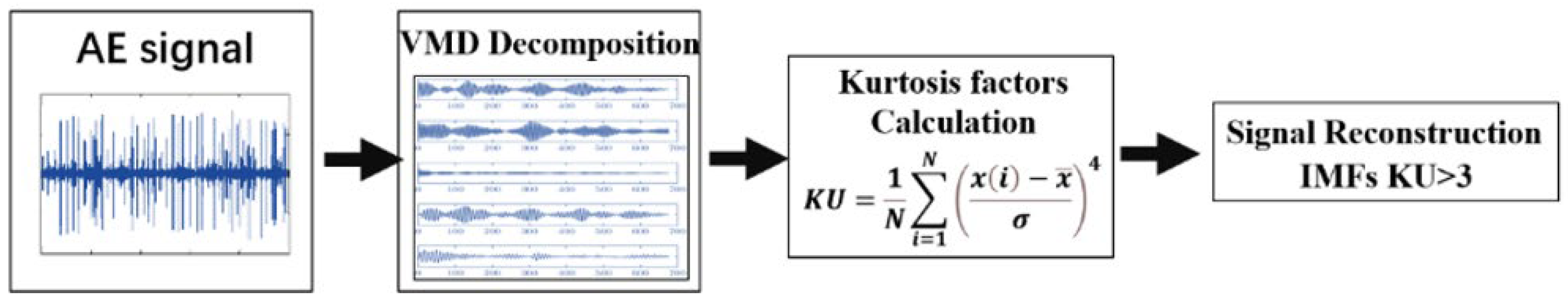
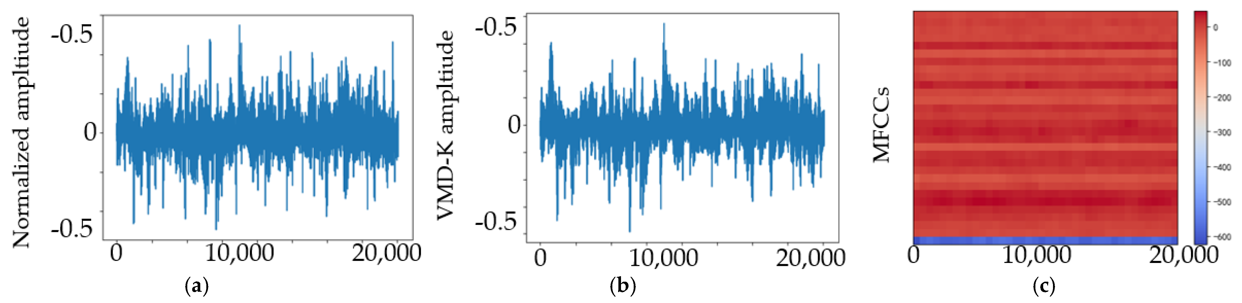
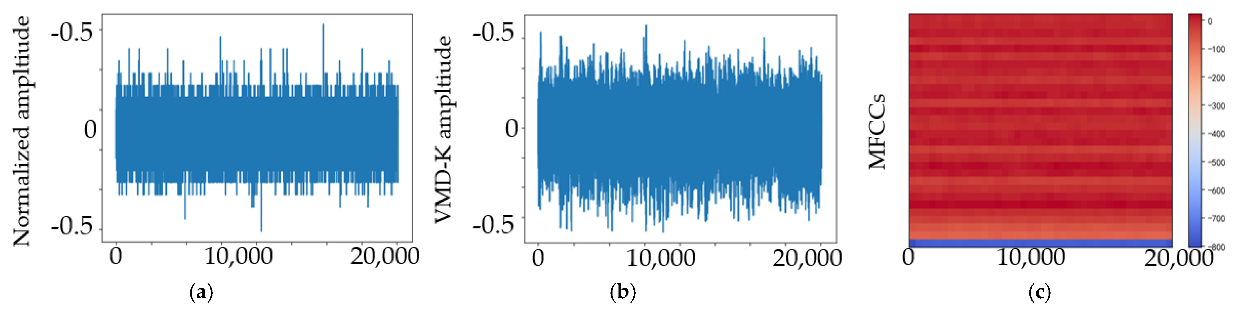
2.1. VMD-Kurtosis Denoising
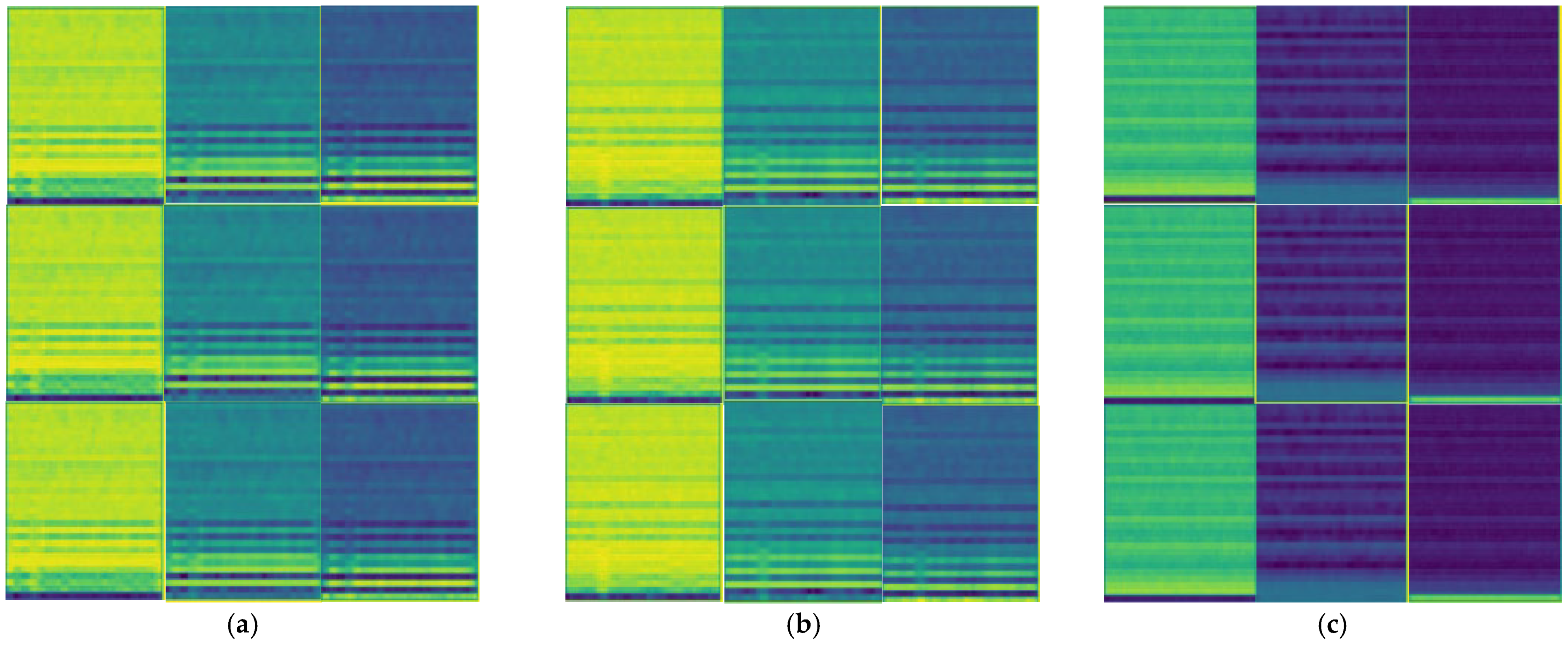
2.2. MFCCs
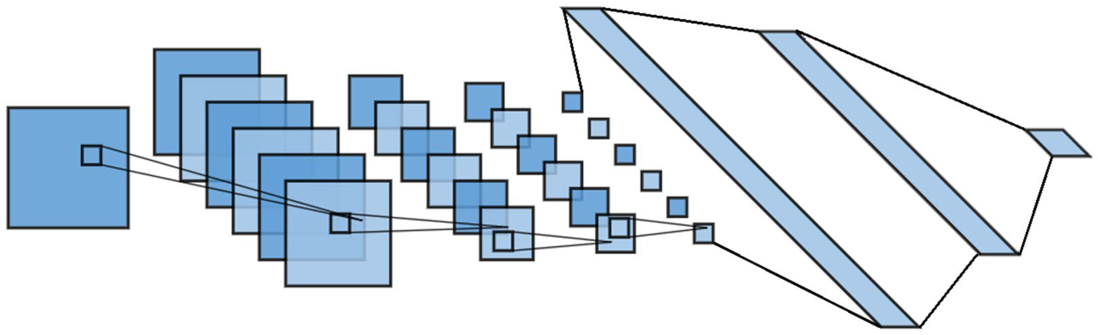
2.3. CNNs
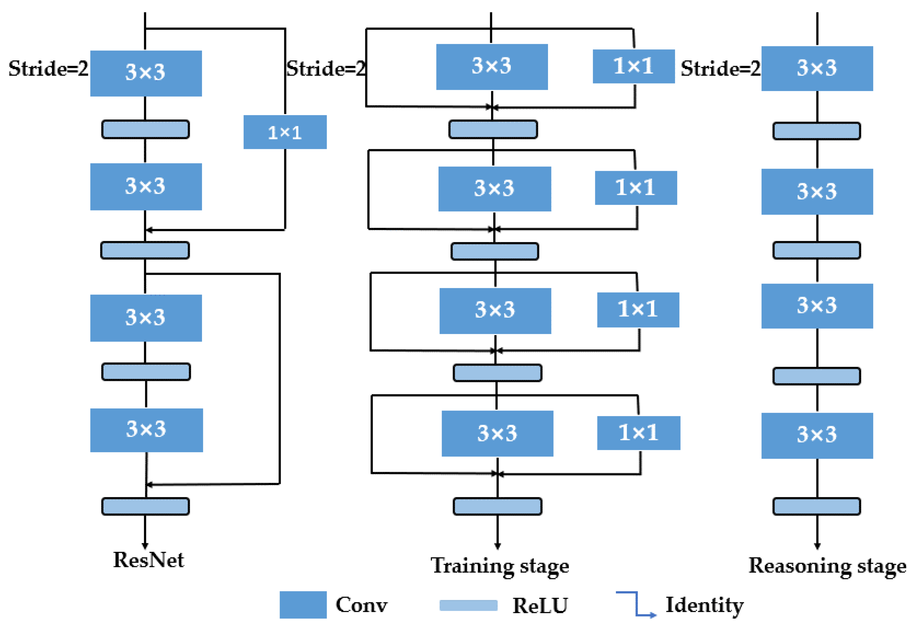
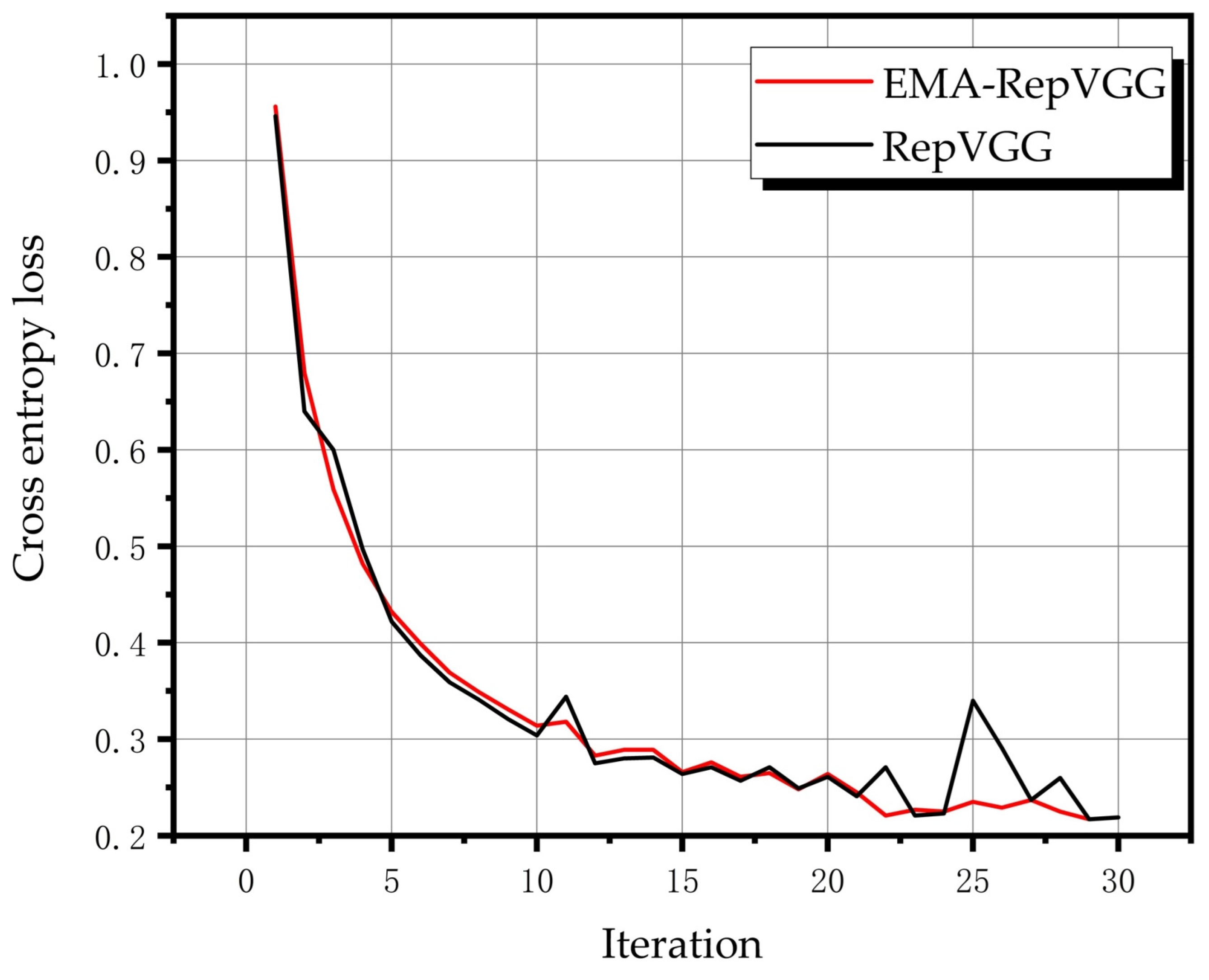
2.4. EMA-RepVGG
3. Experimental Setup and Data Acquisition
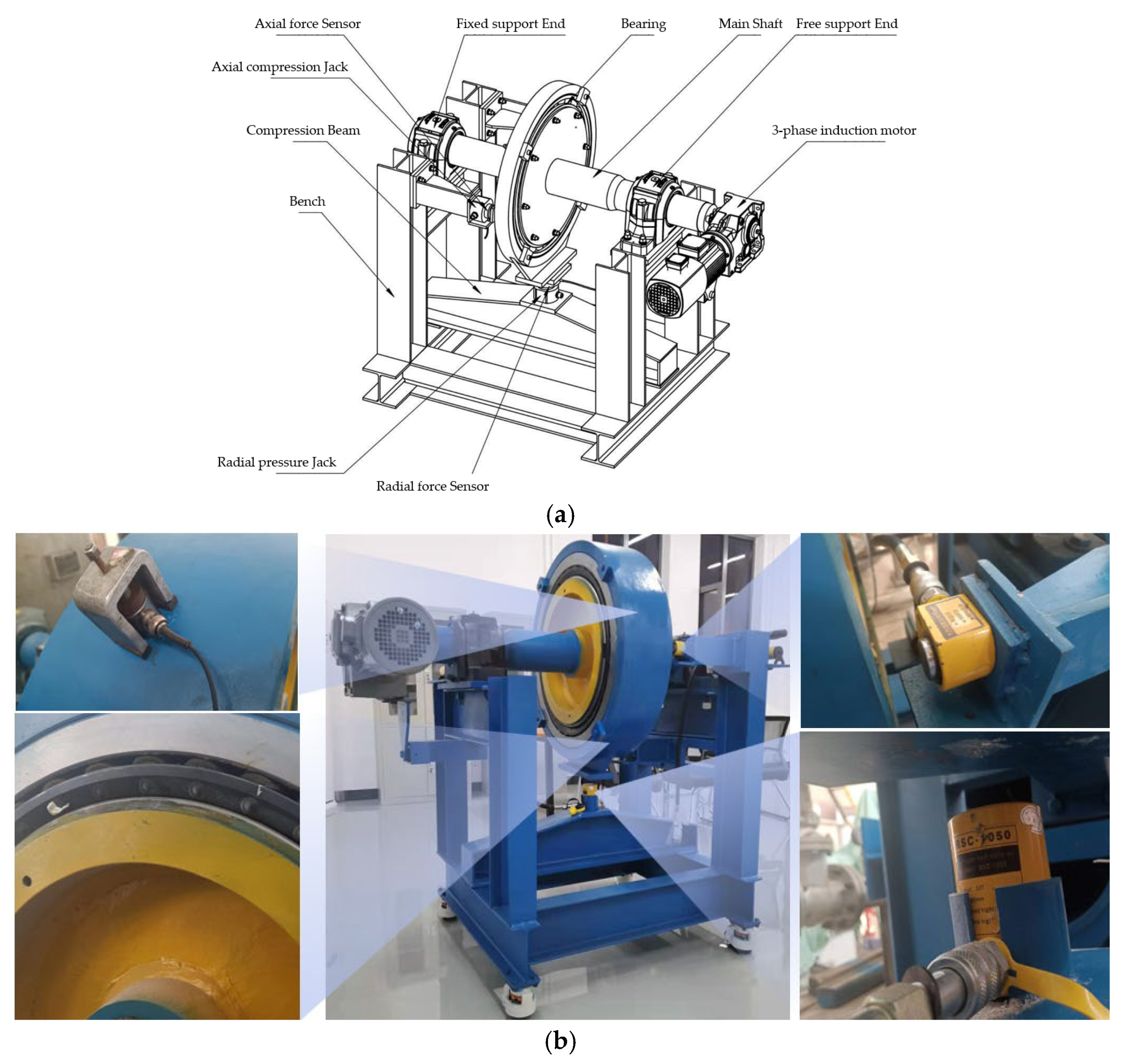
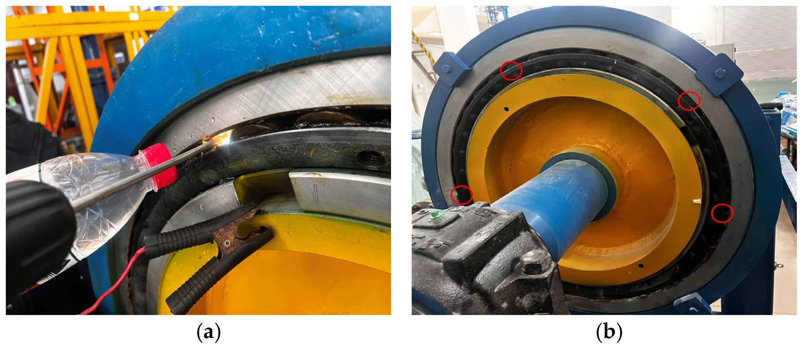
3.1. Bearing Fault Simulator Experiment
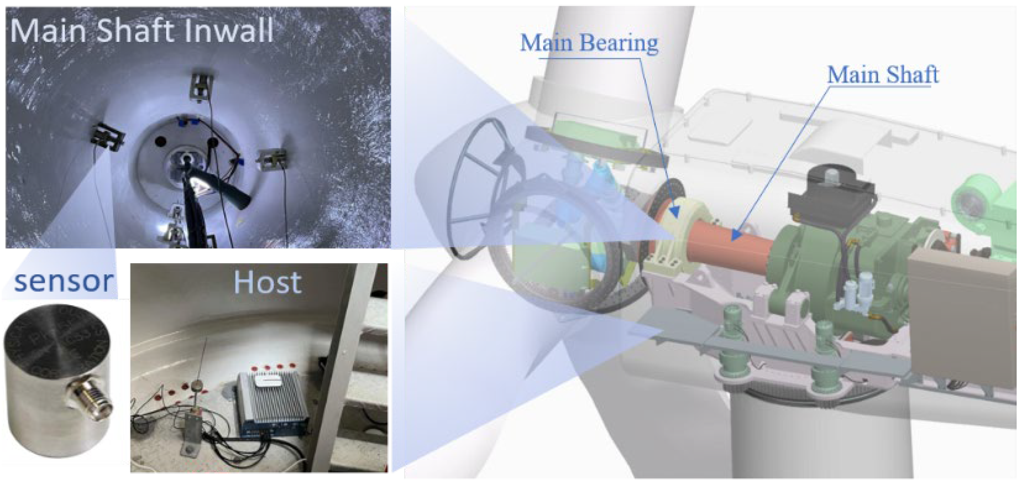
3.2. Wind Turbine Spindle Bearing on-Line Experiment
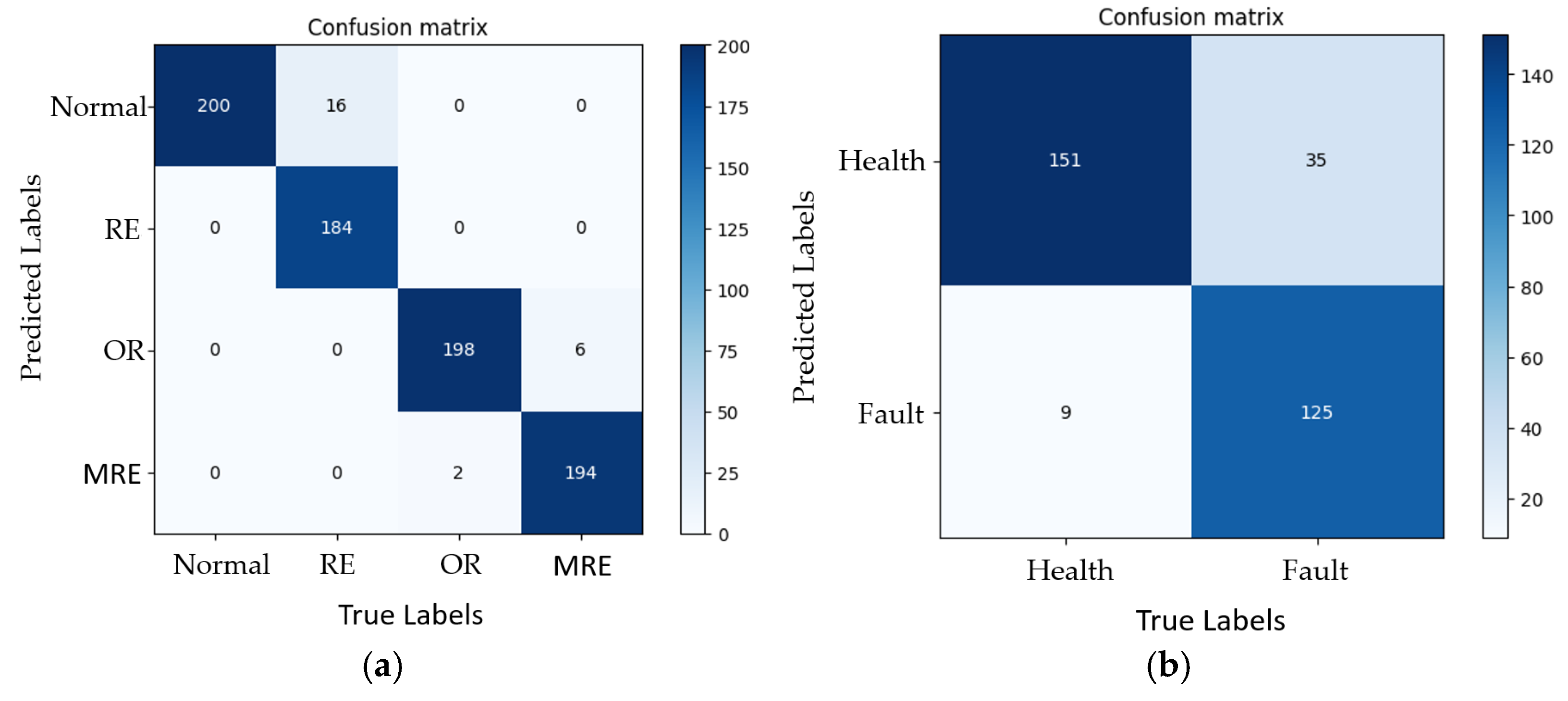
4. Experimental Results and Discussion
5. Conclusions
- AE technology can be employed for the signal acquisition of low-speed heavy load bearings.
- DL CNNs can be used for industrial condition monitoring.
- The EMA-RepVGG model is an industrial application model suitable for remote deployment and embedded development.
- MFCCs focus on low-frequency signals in AE signals, which is beneficial for low-speed bearing failure detection.
- Denoising the model input aids in the optimization of the training process under specific circumstances.
Author Contributions
Funding
Institutional Review Board Statement
Informed Consent Statement
Data Availability Statement
Conflicts of Interest
References
- Rogelj, J.; Schaeffer, M.; Meinshausen, M.; Knutti, R.; Alcamo, J.; Riahi, K.; Hare, W. Zero emission targets as long-term global goals for climate protection. Environ. Res. Lett. 2015, 10, 105007. [Google Scholar] [CrossRef]
- Chen, H.; Chen, J.; Han, G.; Cui, Q. Winding down the wind power curtailment in China: What made the difference? Renew. Sustain. Energy Rev. 2022, 167, 112725. [Google Scholar] [CrossRef]
- Brusa, E. Design of a kinematic vibration energy harvester for a smart bearing with piezoelectric/magnetic coupling. Mech. Adv. Mater. Struct. 2020, 27, 1322–1330. [Google Scholar] [CrossRef]
- Garcia-Calva, T.; Morinigo-Sotelo, D.; Fernandez-Cavero, V.; Romero-Troncoso, R. Early detection of faults in induction motors—A review. Energies 2022, 15, 7855. [Google Scholar] [CrossRef]
- Bharadwaj, S.; Singh, S.; Kumar, R. A review on acoustic emission analysis for bearing fault detection and classification. Measurement 2019, 145, 800–819. [Google Scholar] [CrossRef]
- Ali, Y.H.; Abd Rahman, R.; Hamzah, R.I.R. Acoustic emission signal analysis and artificial intelligence techniques in machine condition monitoring and fault diagnosis: A review. J. Teknol. 2014, 69, 121–126. [Google Scholar] [CrossRef] [Green Version]
- Wu, G.; Yan, T.; Yang, G.; Chai, H.; Cao, C. A review on rolling bearing fault signal detection methods based on different sensors. Sensors 2022, 22, 8330. [Google Scholar] [CrossRef]
- Kim, J.Y.; Kim, J.M. Bearing fault diagnosis using grad-CAM and acoustic emission signals. App. Sci. 2020, 10, 2050. [Google Scholar] [CrossRef] [Green Version]
- Cooley, J.W.; Tukey, J.W. An algorithm for the machine calculation of complex Fourier series. Math. Comput. 1965, 19, 297–301. [Google Scholar] [CrossRef]
- Kraśny, M.J.; Bowen, C.R. A system for characterisation of piezoelectric materials and associated electronics for vibration powered energy harvesting devices. Measurement 2021, 168, 108285. [Google Scholar] [CrossRef]
- Zhang, L.; Zhang, X.; Lu, G. Application of improved Hilbert envelope analysis for incipient fault diagnosis of rolling bearings. Mech. Syst. Signal Process. 2018, 99, 731–747. [Google Scholar] [CrossRef]
- Lu, Q.; Shen, X.; Wang, X.; Li, M.; Li, J.; Zhang, M. Fault diagnosis of rolling bearing based on improved VMD and KNN. Math. Probl. Eng. 2021, 2021, 2530315. [Google Scholar] [CrossRef]
- Baccarini, L.M.R.; e Silva, V.V.R.; de Menezes, B.R.; Caminhas, W.M. SVM practical industrial application for mechanical faults diagnostic. Expert Syst. Appl. 2011, 38, 6980–6984. [Google Scholar] [CrossRef]
- Breiman, L. Random forests. Mach. Learn. 2001, 45, 5–32. [Google Scholar] [CrossRef] [Green Version]
- Rumelhart, D.E.; Hinton, G.E.; Williams, R.J. Learning representations by back-propagating errors. Nature 1986, 323, 533–536. [Google Scholar] [CrossRef]
- Hinton, G.E.; Osindero, S.; Teh, Y.-W. A fast learning algorithm for deep belief nets. Neural Comput. 2006, 18, 1527–1554. [Google Scholar] [CrossRef]
- Grezmak, J.; Zhang, J.; Wang, P.; Loparo, K.A.; Gao, R.X. Interpretable convolutional neural network through layer-wise relevance propagation for machine fault diagnosis. IEEE Sens. J. 2019, 20, 3172–3181. [Google Scholar] [CrossRef]
- Li, G.; Deng, C.; Wu, J.; Chen, Z.; Xu, X. Rolling bearing fault diagnosis based on wavelet packet transform and convolutional neural network. Appl. Sci. 2020, 10, 770. [Google Scholar] [CrossRef] [Green Version]
- Di Maggio, L.G. Intelligent fault diagnosis of industrial bearings using transfer learning and CNNs pre-trained for audio classification. Sensors 2022, 23, 211. [Google Scholar] [CrossRef]
- Smith, W.A.; Randall, R.B. Rolling element bearing diagnostics using the Case Western Reserve University data: A benchmark study. Mech. Syst. Signal Process. 2015, 64, 100–131. [Google Scholar] [CrossRef]
- Hendriks, J.; Dumond, P.; Knox, D.A. Towards better benchmarking using the CWRU bearing fault dataset. Mech. Syst. Signal Process. 2022, 169, 108732. [Google Scholar] [CrossRef]
- Ding, X.; Zhang, X.; Ma, N.; Han, J.; Ding, G.; Sun, J. RepVGG: Making VGG-style ConvNets Great Again. arXiv 2021, arXiv:2101.03697. [Google Scholar] [CrossRef]
- Dragomiretskiy, K.; Zosso, D. Variational mode decomposition. IEEE Trans. Signal Process. 2013, 62, 531–544. [Google Scholar] [CrossRef]
- Westfall, P.H. Kurtosis as peakedness, 1905–2014. RIP. Am. Stat. 2014, 68, 191–195. [Google Scholar] [CrossRef] [PubMed] [Green Version]
- Gu, X.; Yang, S.; Liu, Y.; Hao, R. Rolling element bearing faults diagnosis based on kurtogram and frequency domain correlated kurtosis. Meas. Sci. Technol. 2016, 27, 125019. [Google Scholar] [CrossRef]
- Davis, S.; Mermelstein, P. Comparison of parametric representations for monosyllabic word recognition in continuously spoken sentences. IEEE Trans. Acoust. Speech Signal Process. 1980, 28, 357–366. [Google Scholar] [CrossRef] [Green Version]
- Cai, R.; Wang, Q.; Hou, Y.; Liu, H. Event monitoring of transformer discharge sounds based on voiceprint. J. Phys. Conf. Ser. 2021, 2078, 012066. [Google Scholar] [CrossRef]
- Shi, L.; Ahmad, I.; He, Y.; Chang, K. Hidden Markov model based drone sound recognition using MFCC technique in practical noisy environments. J. Commun. Netw. 2018, 20, 509–518. [Google Scholar] [CrossRef]
- Krizhevsky, A.; Sutskever, I.; Hinton, G.E. Imagenet classification with deep convolutional neural networks. In Proceedings of the Advances in Neural Information Processing Systems 25 (NIPS 2012), Lake Tahoe, NV, USA, 3–6 December 2012; pp. 1097–1105. [Google Scholar]
- LeCun, Y.; Boser, B.; Denker, J.; Henderson, D.; Howard, R.; Hubbard, W.; Jackel, L. Handwritten digit recognition with a back-propagation network. In Proceedings of the Advances in Neural Information Processing Systems 25 (NIPS 2012), Denver, CO, USA, 27–30 November 1989; pp. 396–404. [Google Scholar]
- Zhao, R.; Yan, R.; Chen, Z.; Mao, K.; Wang, P.; Gao, R.X. Deep learning and its applications to machine health monitoring. Mech. Syst. Signal Process. 2019, 115, 213–237. [Google Scholar] [CrossRef]
- Lei, Y.; Yang, B.; Jiang, X.; Jia, F.; Li, N.; Nandi, A.K. Applications of machine learning to machine fault diagnosis: A review and roadmap. Mech. Syst. Signal Process. 2020, 138, 106587. [Google Scholar] [CrossRef]
- Girshick, R.; Donahue, J.; Darrell, T.; Malik, J. Rich feature hierarchies for accurate object detection and semantic segmentation. In Proceedings of the IEEE Conference on Computer Vision and Pattern Recognition, Columbus, OH, USA, 23–28 June 2014; pp. 580–587. [Google Scholar]
- Lecun, Y.; Bottou, L.; Bengio, Y.; Haffner, P. Gradient-based learning applied to document recognition. Proc. IEEE 1998, 86, 2278–2324. [Google Scholar] [CrossRef] [Green Version]
- Liu, Y.; Zhang, C.; Hang, B.; Wang, S.; Chao, H.-C. An audio attention computational model based on information entropy of two channels and exponential moving average. Hum. Cent. Comput. Inf. Sci. 2019, 9, 7. [Google Scholar] [CrossRef] [Green Version]
- Bottou, L. Stochastic Gradient Descent Tricks. In Neural Networks: Tricks of the Trade; Springer: Berlin/Heidelberg, Germany, 2012; pp. 421–436. [Google Scholar] [CrossRef] [Green Version]
- Kingma, D.P.; Ba, J.L. Adam: A Method for Stochastic Optimization. In Proceedings of the 3rd International Conference on Learning Representations, ICLR 2015, San Diego, CA, USA, 7–9 May 2015; pp. 1–15. [Google Scholar]
- He, K.; Zhang, X.; Ren, S.; Sun, J. Deep residual learning for image recognition. In Proceedings of the 2016 IEEE Conference on Computer Vision and Pattern Recognition (CVPR), Las Vegas, NV, USA, 27–30 June 2016; pp. 770–778. [Google Scholar]
- Tan, M.; Le, Q.V. EfficientNet: Rethinking model scaling for convolutional neural networks. arXiv 2019, arXiv:1905.11946. [Google Scholar] [CrossRef]


| Hyperparameters | Value |
|---|---|
| Optimizer | Adam [37] |
| L2 regularization | 1 × 10⁻⁶ |
| Mini batch size | 32 |
| Initial learning rate | 5 × 10⁻⁴ |
| Max epochs | 30 |
| 0.999 |
| Bearing Outer Diameter D | Bearing Inner Diameter d | Thickness | Number of Rolling Elements | Contact Angle |
|---|---|---|---|---|
| 733.4 mm | 509.94 mm | 200 mm | 2 × 35 | 45° |
| Project | Channel | Threshold (dB) | PDT (μs) | HDT (μs) | HLT (μs) |
|---|---|---|---|---|---|
| parameter | 4 | 35 | 1000 | 2000 | 2000 |
| Load Case 1 | Load Case 1 | Load Case 1 | Load Case 1 | |
|---|---|---|---|---|
| Radial load (kN) | 0 | 50 | 100 | 100 |
| Axial load (kN) | 0 | 0 | 0 | 50 |
| Nominal speeds (rpm) | 5, 10, 15, 20 | |||
| Total acquisition duration (s) | 10 |
| Sampling frequency (Hz) | 25,000 |
| Chunk length (samples) | 25,000 |
| Chunk length (s) | 1.0 |
| Number of chunks per signal | 10 |
| Classes | Label | Training Samples (80%) | Validation Samples (10%) | Test Samples (10%) |
|---|---|---|---|---|
| 4 | Normal | 1600 | 200 | 200 |
| IR | 1600 | 200 | 200 | |
| OR | 1600 | 200 | 200 | |
| RE | 1600 | 200 | 200 | |
| Total | 8000 | 800 | 800 |
| Model | Training Accuracy | Test Accuracy | Training Time (s) | Reasoning Time (s) | Peak Memory Allocated (MB) |
|---|---|---|---|---|---|
| EMA-RepVGG with MFCCs | 98.88% | 97.57% | 1611 | 9.08 | 305 |
| EMA-RepVGG with FFT | 95.46% | 95.05% | 1688 | 9.12 | 305 |
| EMA-RepVGG without VMD-Kurtosis Denoising | 91.48% | 92.68% | 1679 | 9.49 | 305 |
| ResNet [38] | 96.44% | 96.25% | 4640 | 15.27 | 477 |
| EfficientNet V1 [39] | 90.12% | 92.96% | 1501 | 13.99 | 430 |
| Model | Label | Precision | Recall | Specificity |
|---|---|---|---|---|
| EMA-RepVGG with MFCCs | Normal | 93.1% | 100% | 97.9% |
| ER | 100% | 92.3% | 100% | |
| OR | 97.0% | 99.2% | 99.1% | |
| MER | 99.3% | 97.3% | 99.8% | |
| EMA-RepVGG with FFT | Normal | 90.8% | 93.2% | 92.1% |
| ER | 91.7% | 91.6% | 94.7% | |
| OR | 91.3% | 92.7% | 93.2% | |
| MER | 93.4% | 94.1% | 94.1% | |
| EMA-RepVGG without VMD-Kurtosis Denoising | Normal | 89.1% | 90.8% | 92.6% |
| ER | 92.6% | 88.9% | 89.7% | |
| OR | 92.4% | 89.7% | 91.3% | |
| MER | 93.4% | 91.7% | 93.4% | |
| ResNet 50 [38] | Normal | 94.4% | 92.0% | 98.2% |
| ER | 100% | 94.5% | 100% | |
| OR | 99.0% | 99.0% | 99.7% | |
| MER | 92.1% | 99.5% | 97.2% | |
| EfficientNet V1 [39] | Normal | 91.3% | 93.9% | 97.0% |
| ER | 93.5% | 90.7% | 98.0% | |
| OR | 93.9% | 92.5% | 98.1% | |
| MER | 93.4% | 94.6% | 97.5% |
Disclaimer/Publisher’s Note: The statements, opinions and data contained in all publications are solely those of the individual author(s) and contributor(s) and not of MDPI and/or the editor(s). MDPI and/or the editor(s) disclaim responsibility for any injury to people or property resulting from any ideas, methods, instructions or products referred to in the content. |
© 2023 by the authors. Licensee MDPI, Basel, Switzerland. This article is an open access article distributed under the terms and conditions of the Creative Commons Attribution (CC BY) license (https://creativecommons.org/licenses/by/4.0/).
Share and Cite
Jiang, P.; Sun, W.; Li, W.; Wang, H.; Liu, C. Extreme-Low-Speed Heavy Load Bearing Fault Diagnosis by Using Improved RepVGG and Acoustic Emission Signals. Sensors 2023, 23, 3541. https://doi.org/10.3390/s23073541
Jiang P, Sun W, Li W, Wang H, Liu C. Extreme-Low-Speed Heavy Load Bearing Fault Diagnosis by Using Improved RepVGG and Acoustic Emission Signals. Sensors. 2023; 23(7):3541. https://doi.org/10.3390/s23073541
Chicago/Turabian StyleJiang, Peng, Wenyu Sun, Wei Li, Hongyu Wang, and Cong Liu. 2023. "Extreme-Low-Speed Heavy Load Bearing Fault Diagnosis by Using Improved RepVGG and Acoustic Emission Signals" Sensors 23, no. 7: 3541. https://doi.org/10.3390/s23073541