
Self-Sensing Rubber for Bridge Bearing Monitoring
 , , , ,
Abstract
:1. Introduction
2. Specimens and Experimental Setup
2.1. Compounds
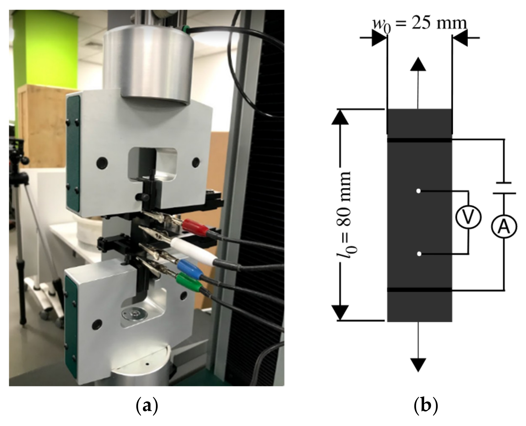
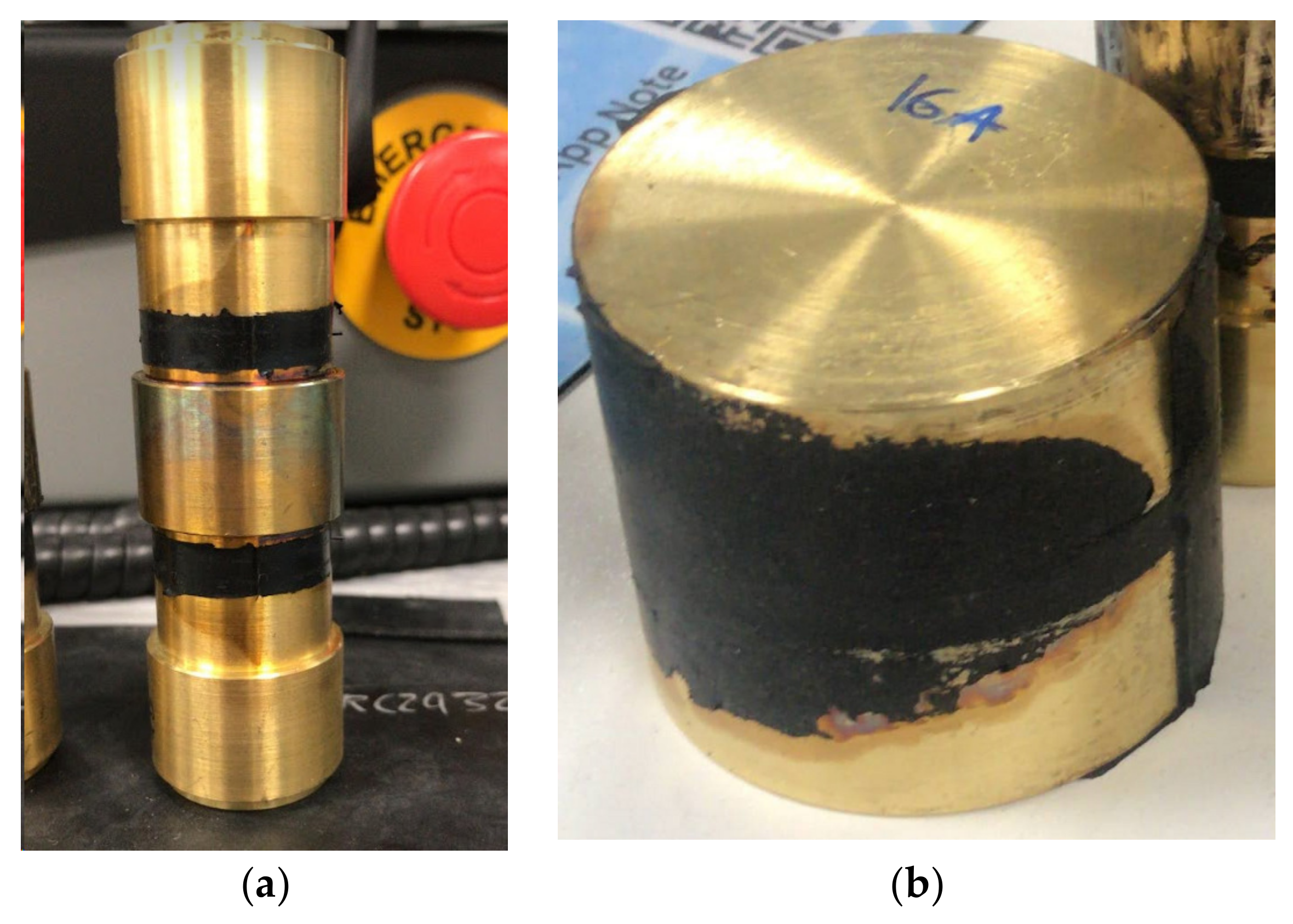
2.2. Test Pieces
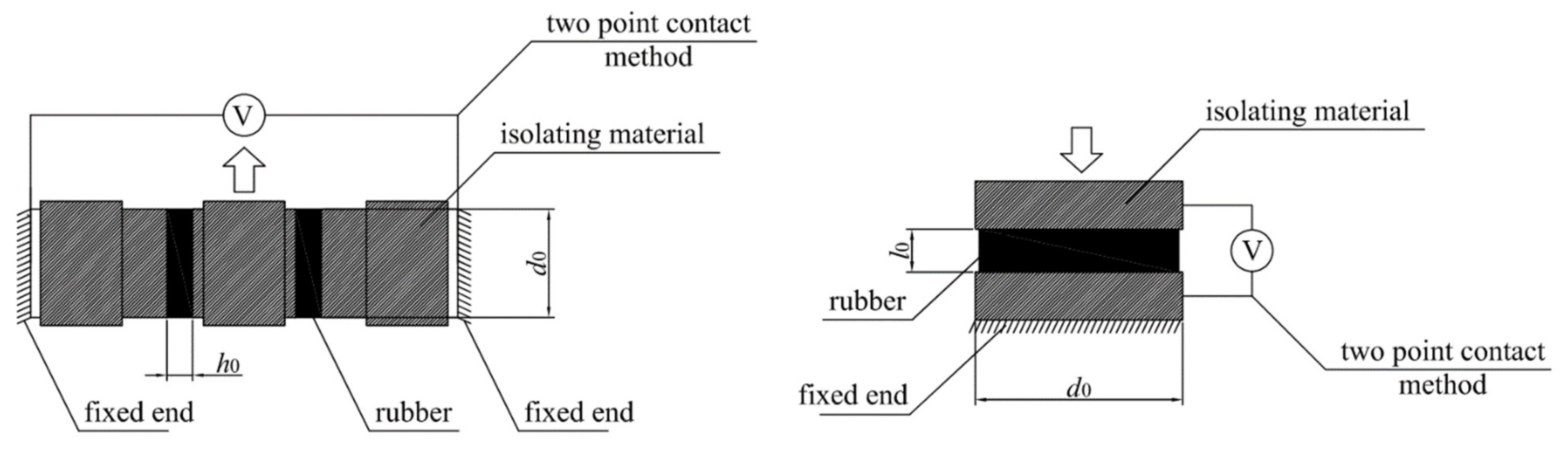
2.3. Stress-Strain Response and Resistivity Measurement
3. Experimental Tests on Rubber Filled with Carbon Black
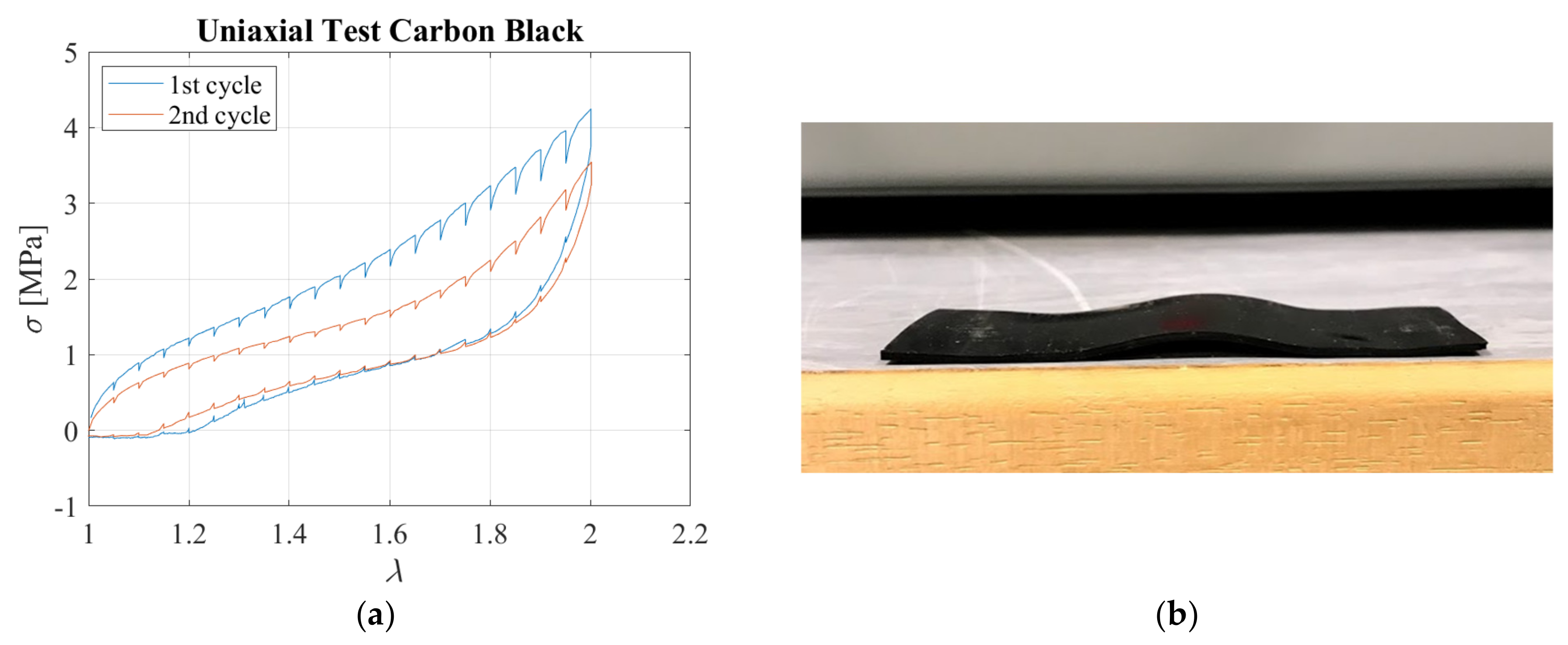
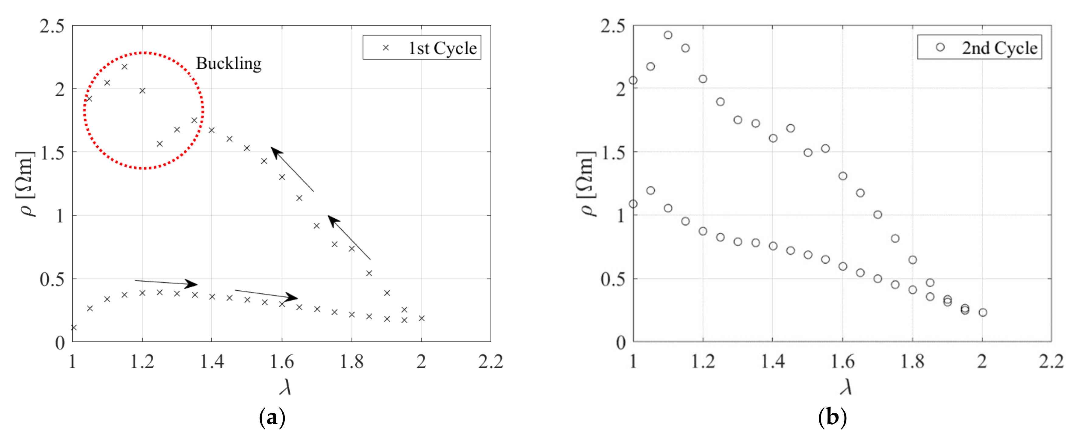
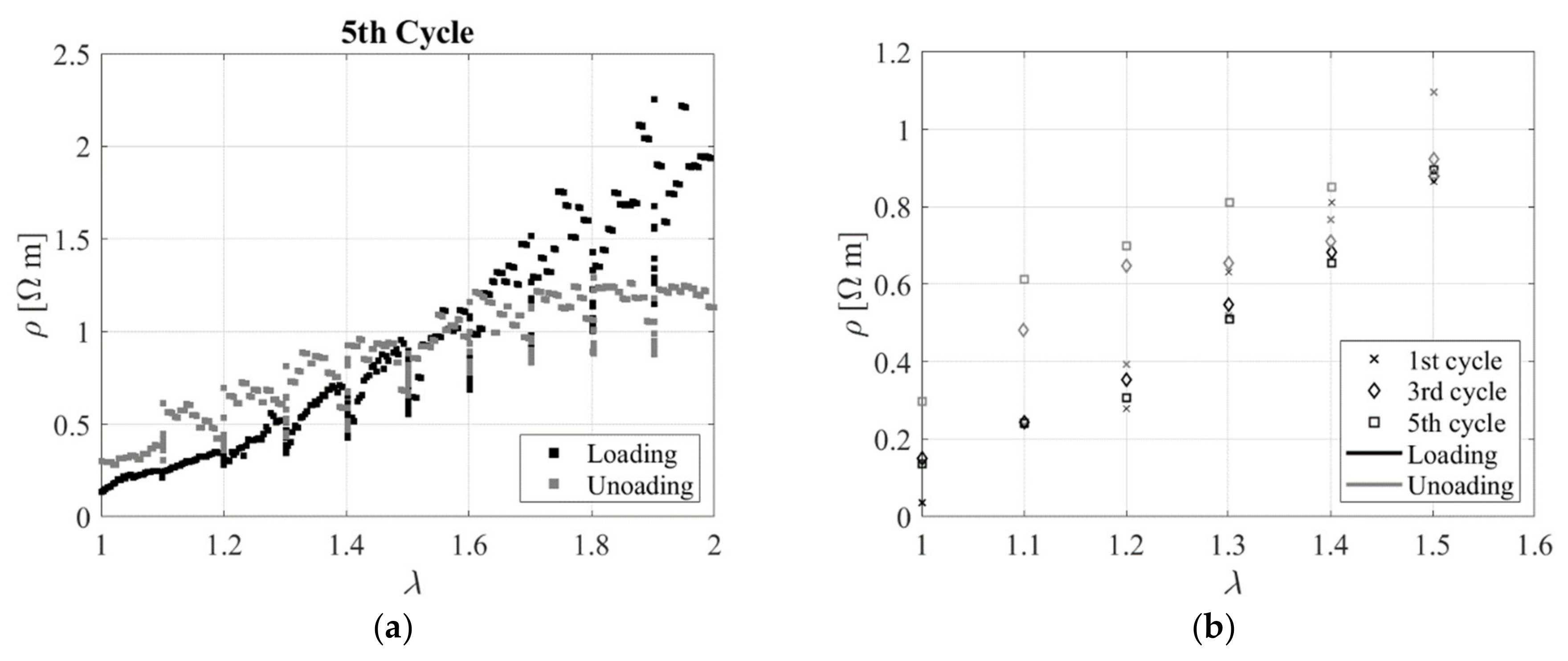
3.1. Full Cyclic Uniaxial Tensile Tests
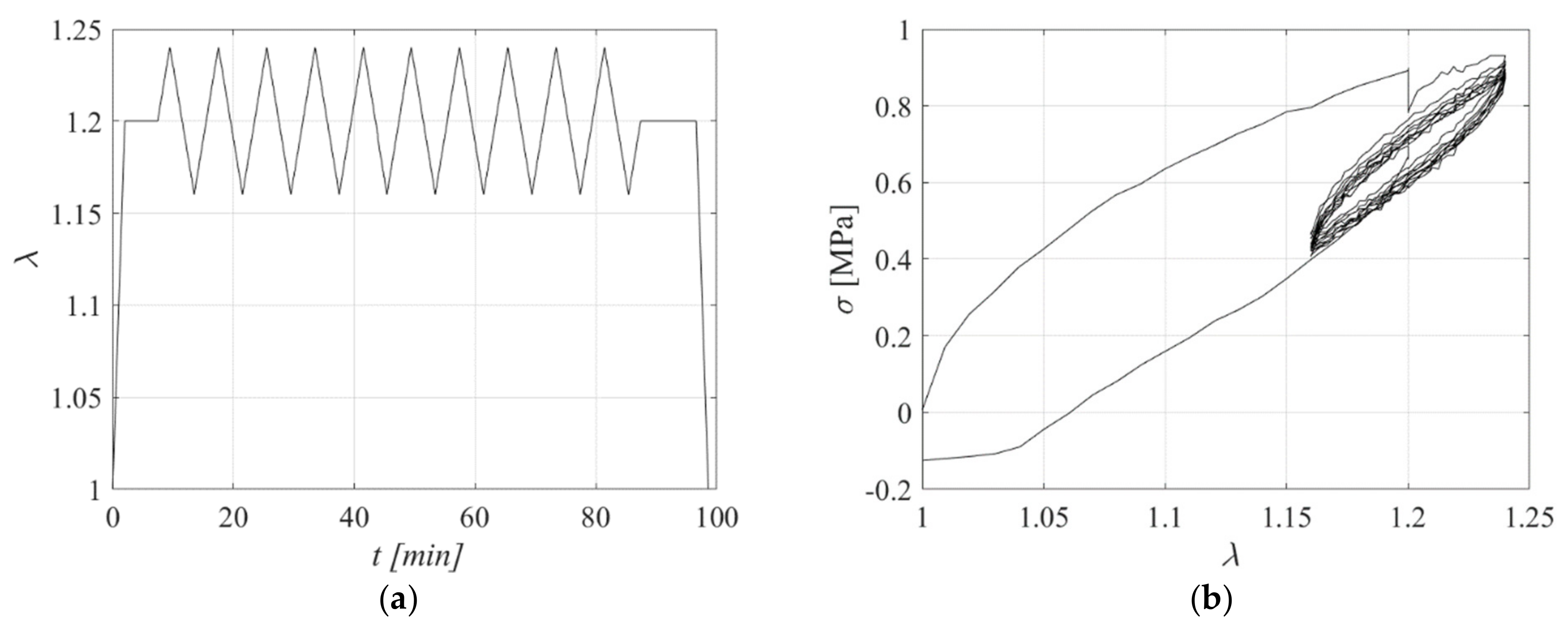
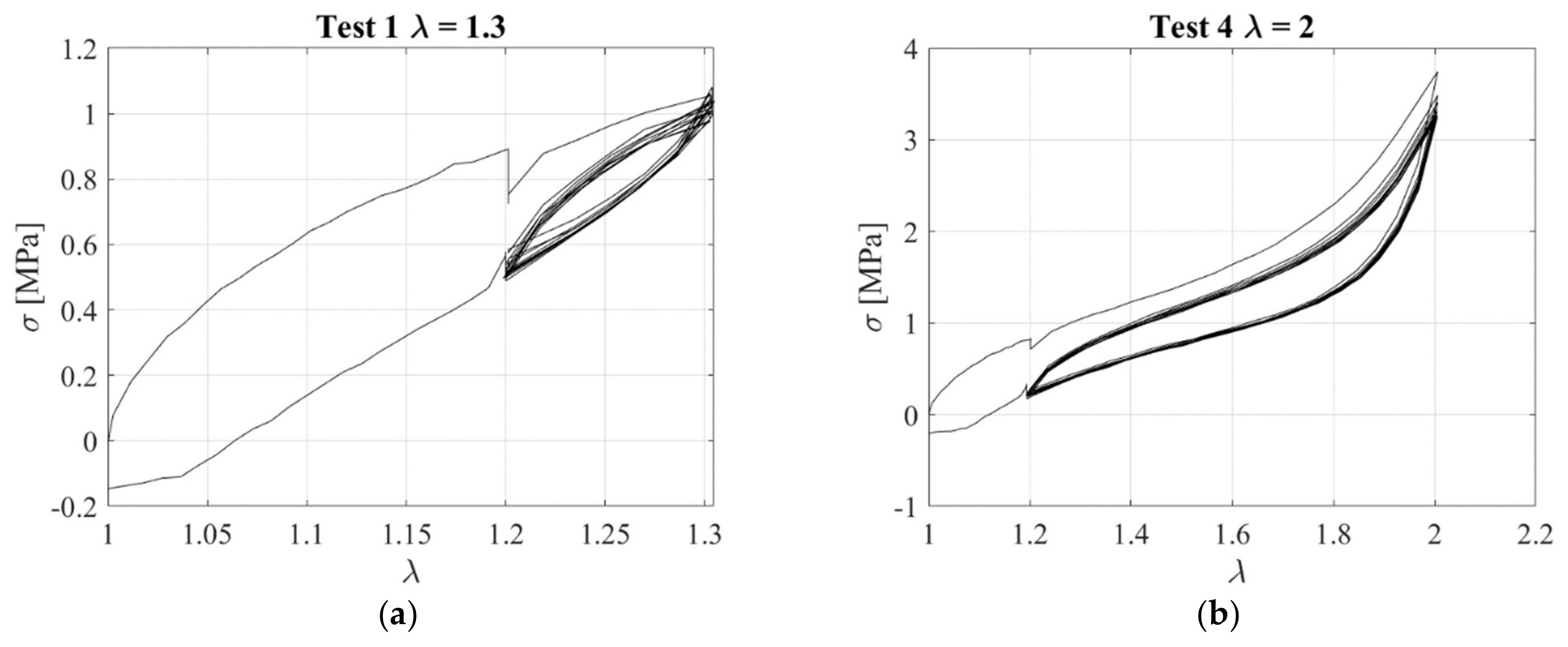
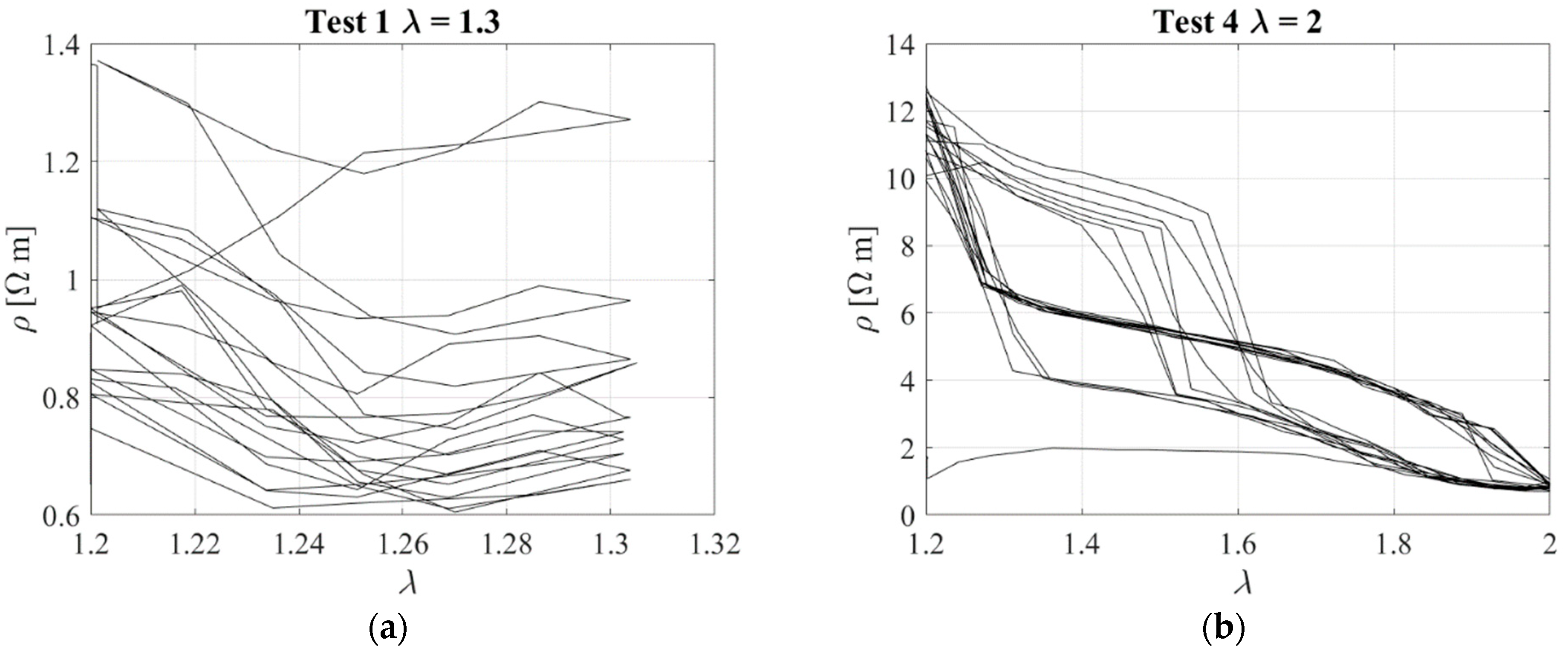
3.2. Uniaxial Tensile Tests: Triangular Input
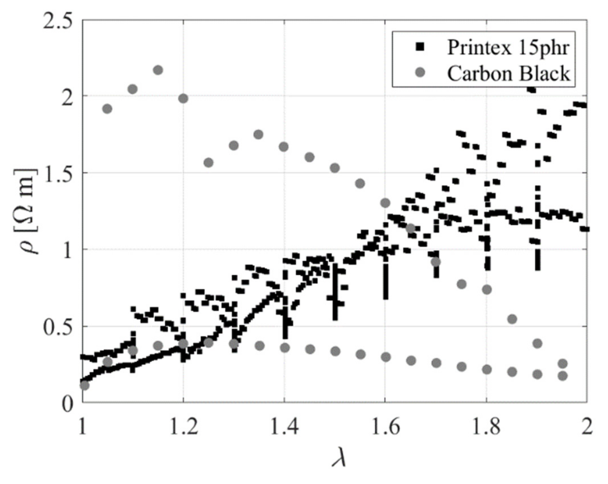
4. Experimental Tests on Rubber Filled with Printex 15 Phr
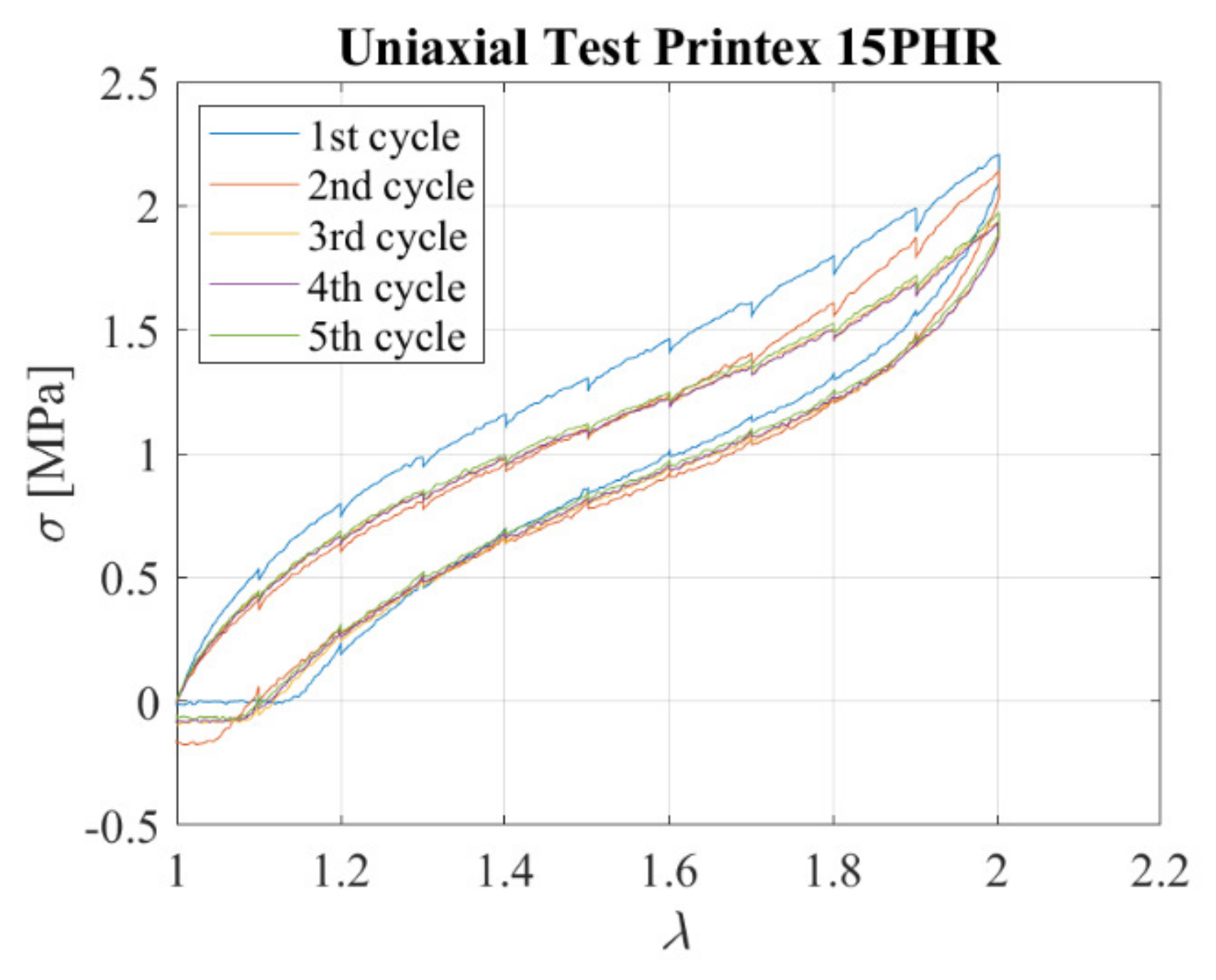
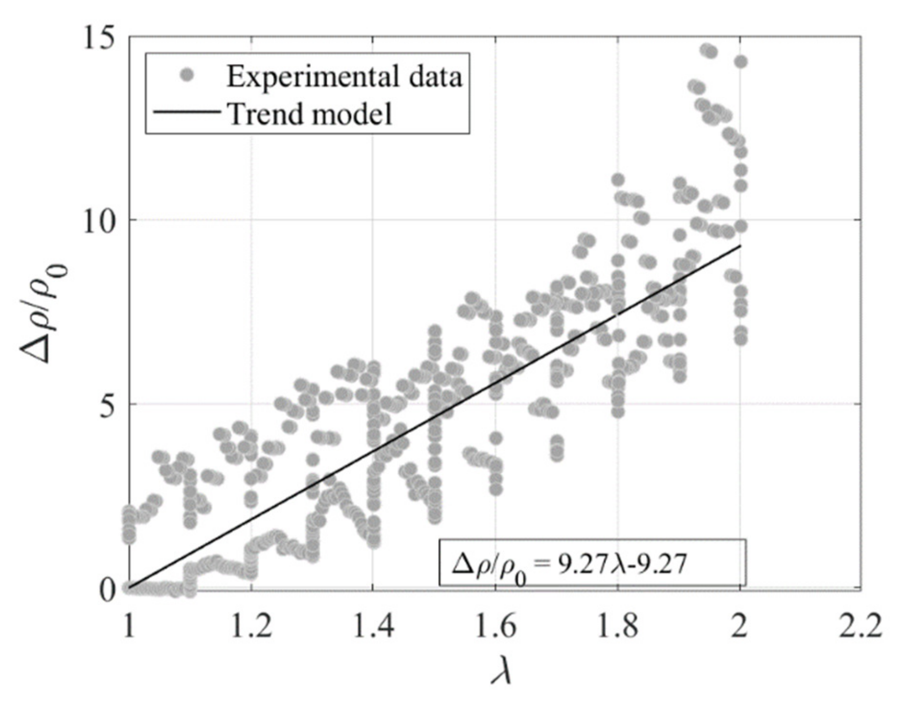
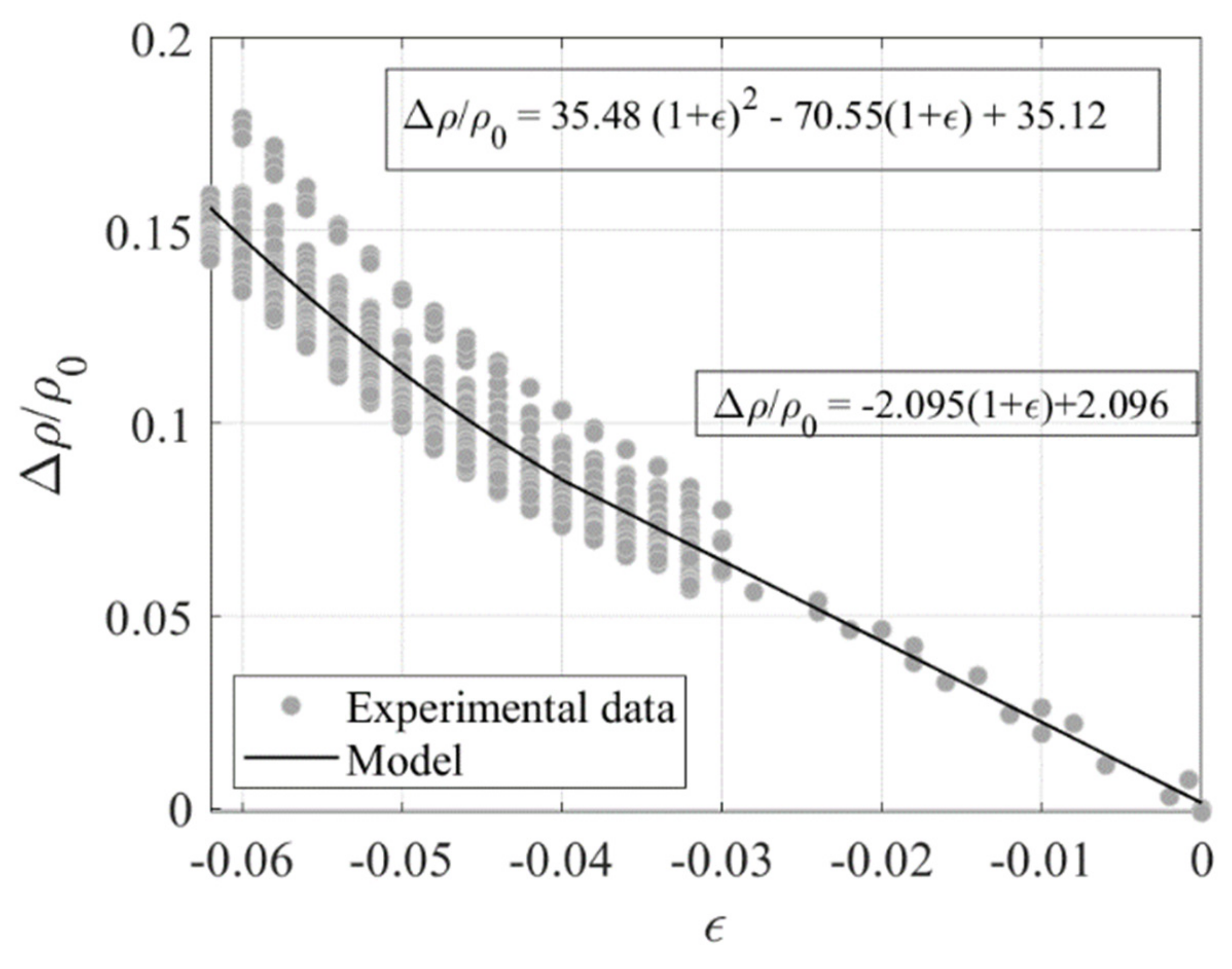
4.1. Uniaxial Tensile Tests
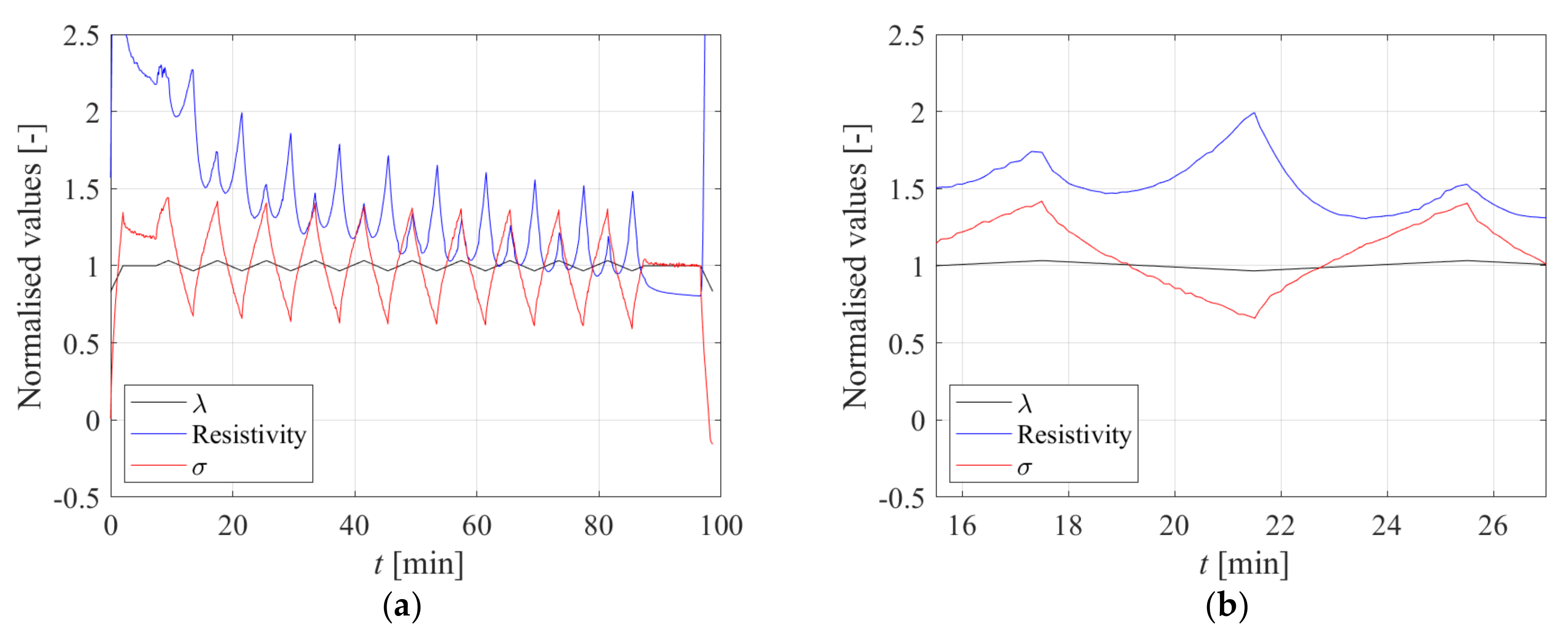
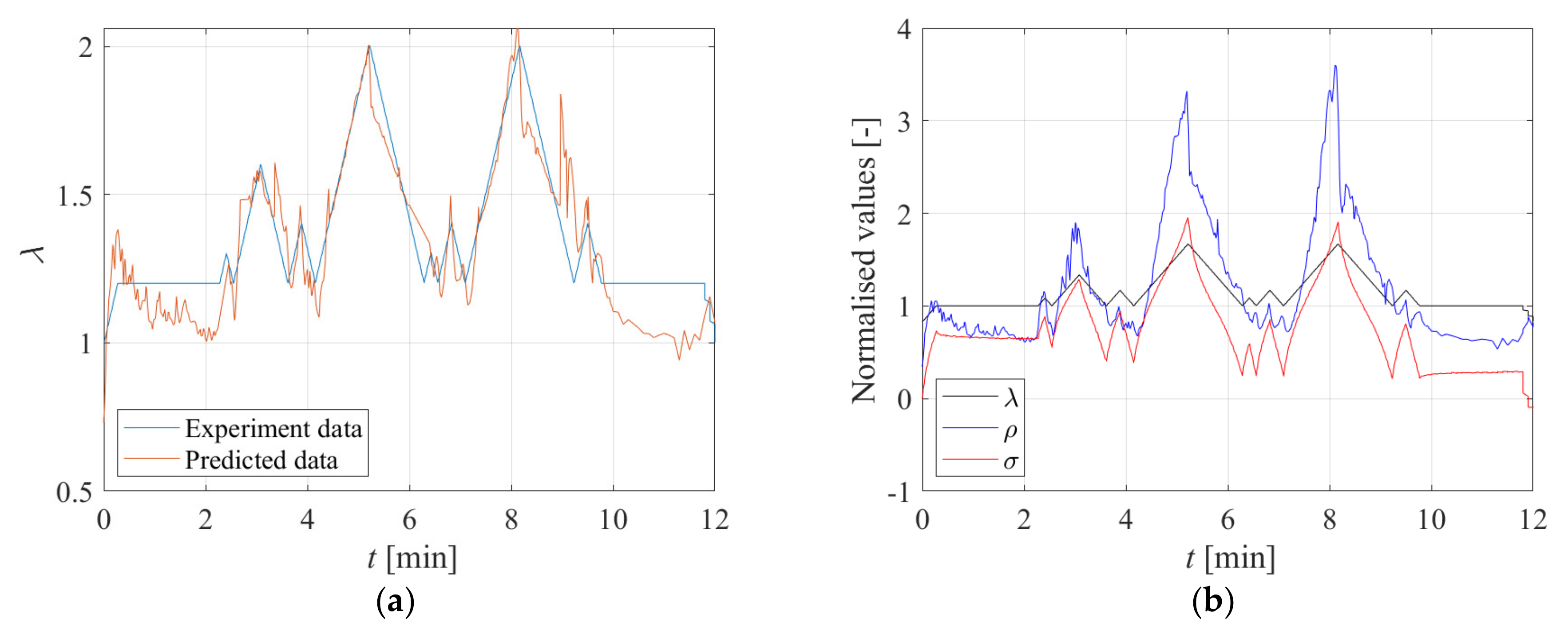
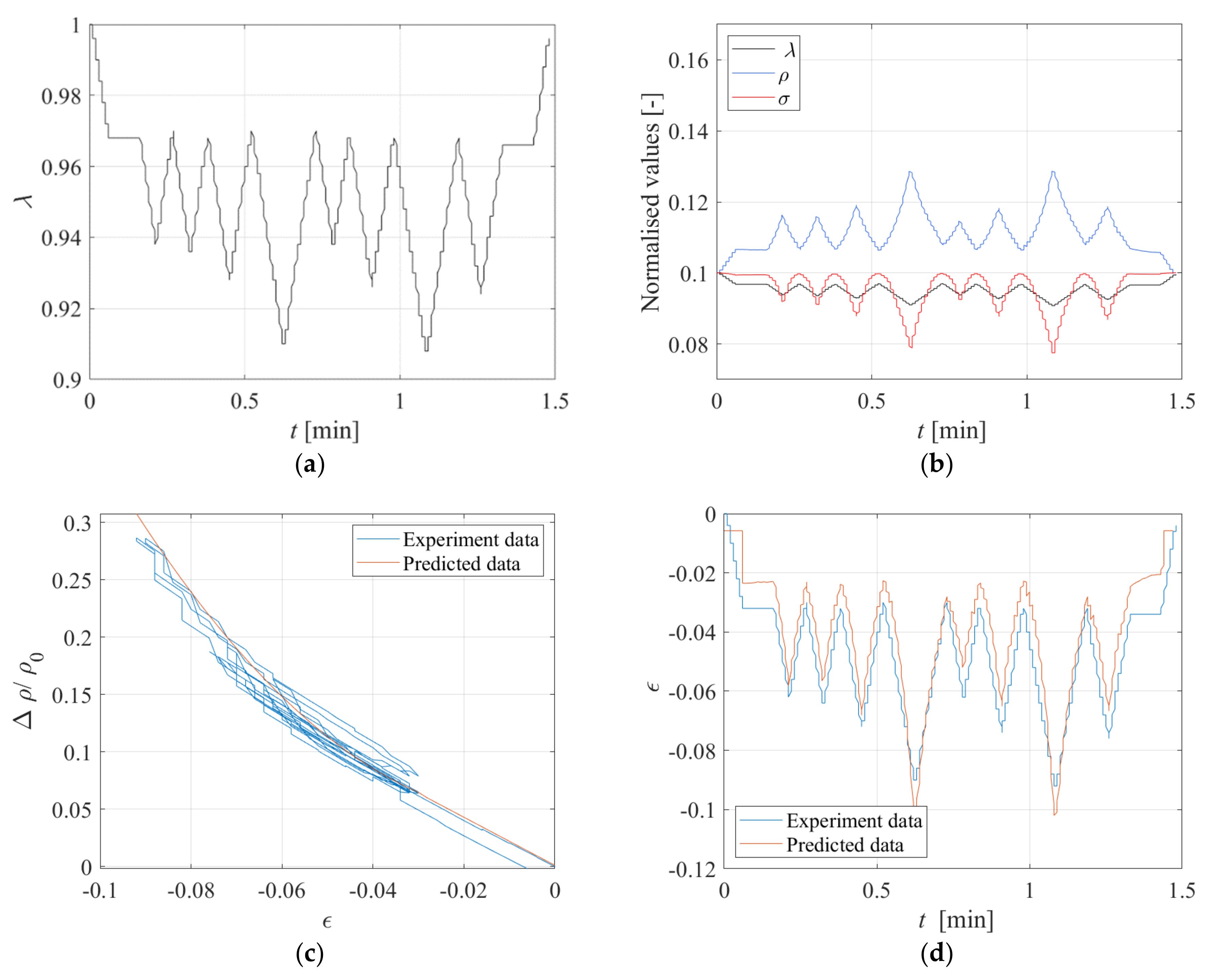
4.2. Uniaxial Tensile Test: Random Input
5. Experimental Tests on Rubber Filled with Printex 12 Phr
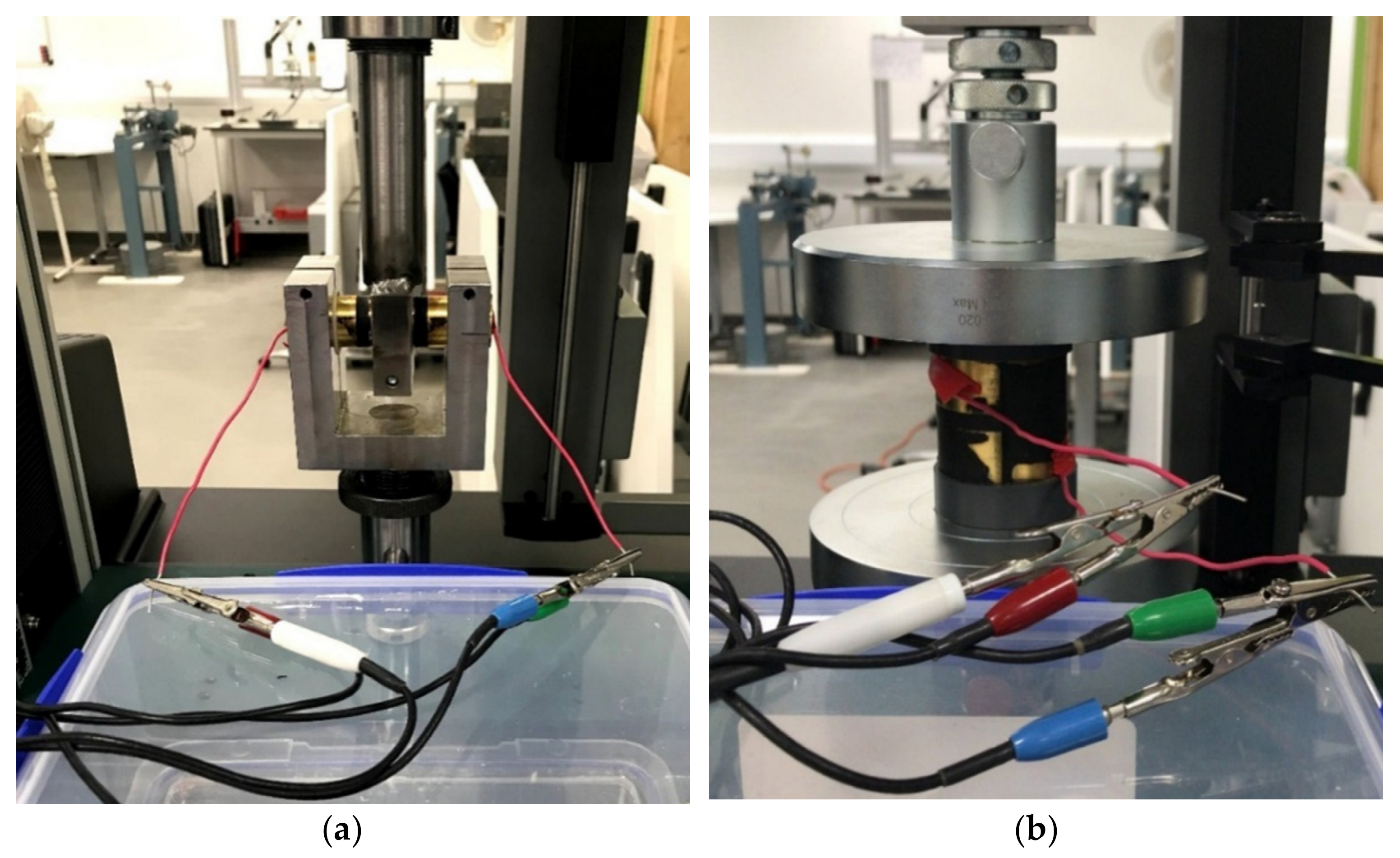
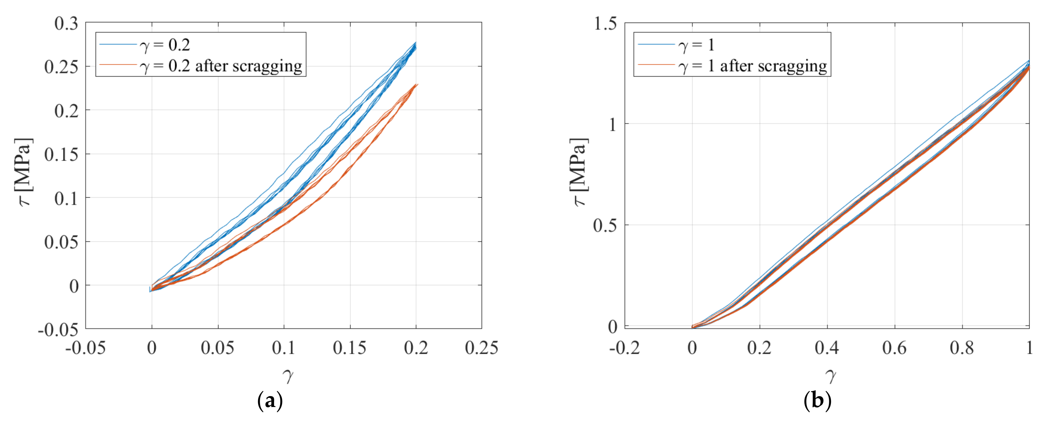
5.1. Double Bonded Shear (DBS) Tests
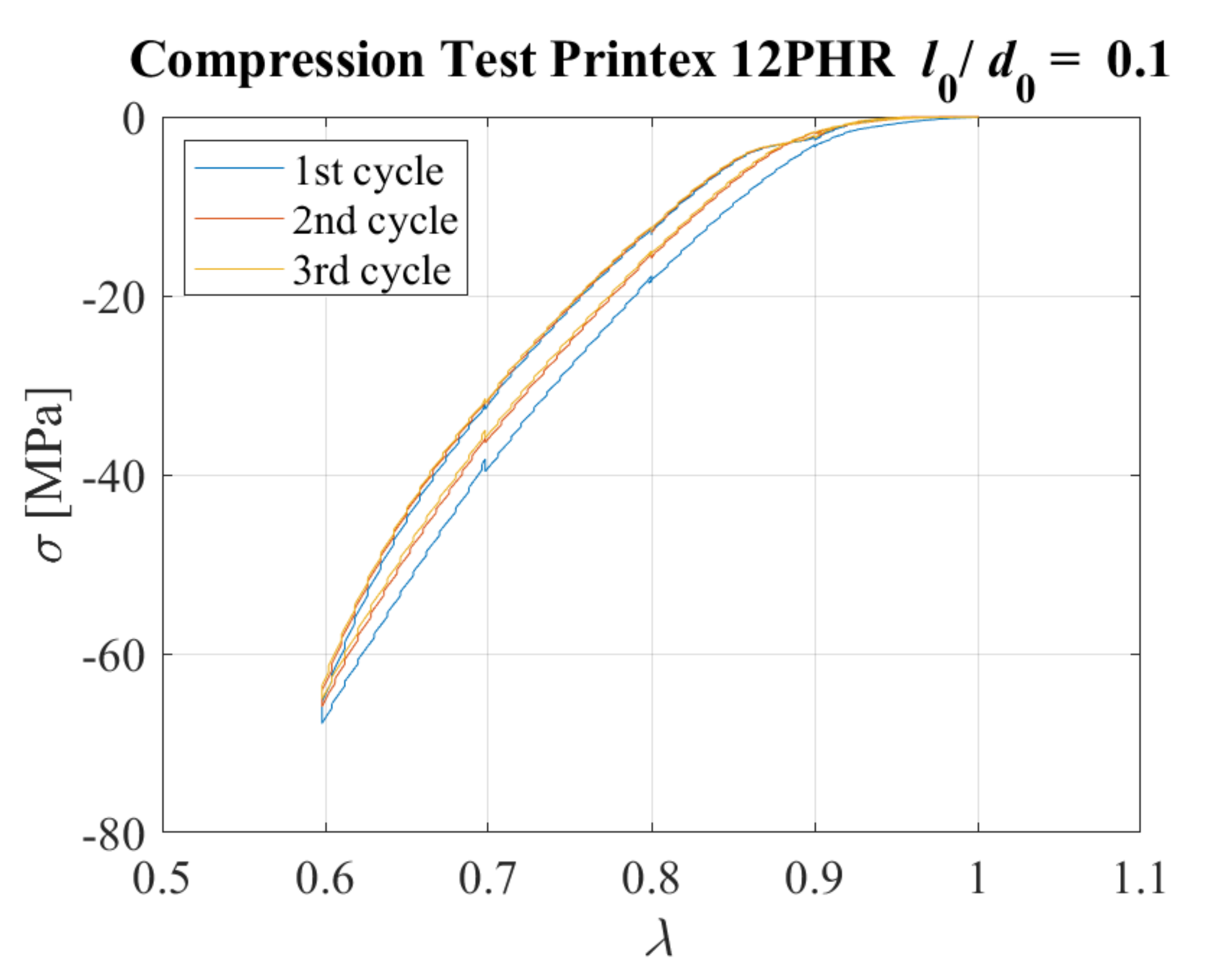
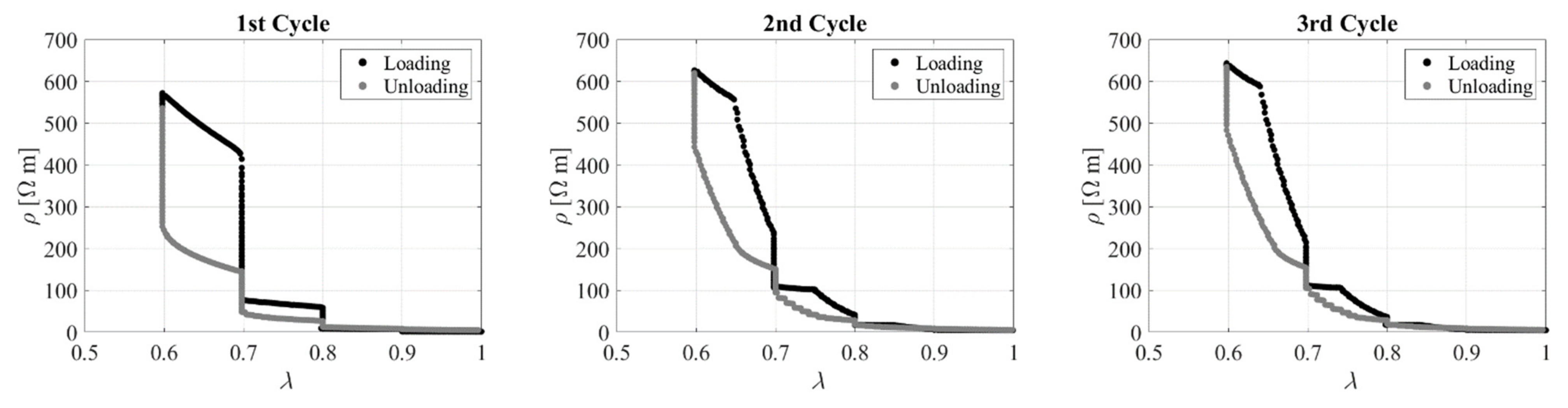
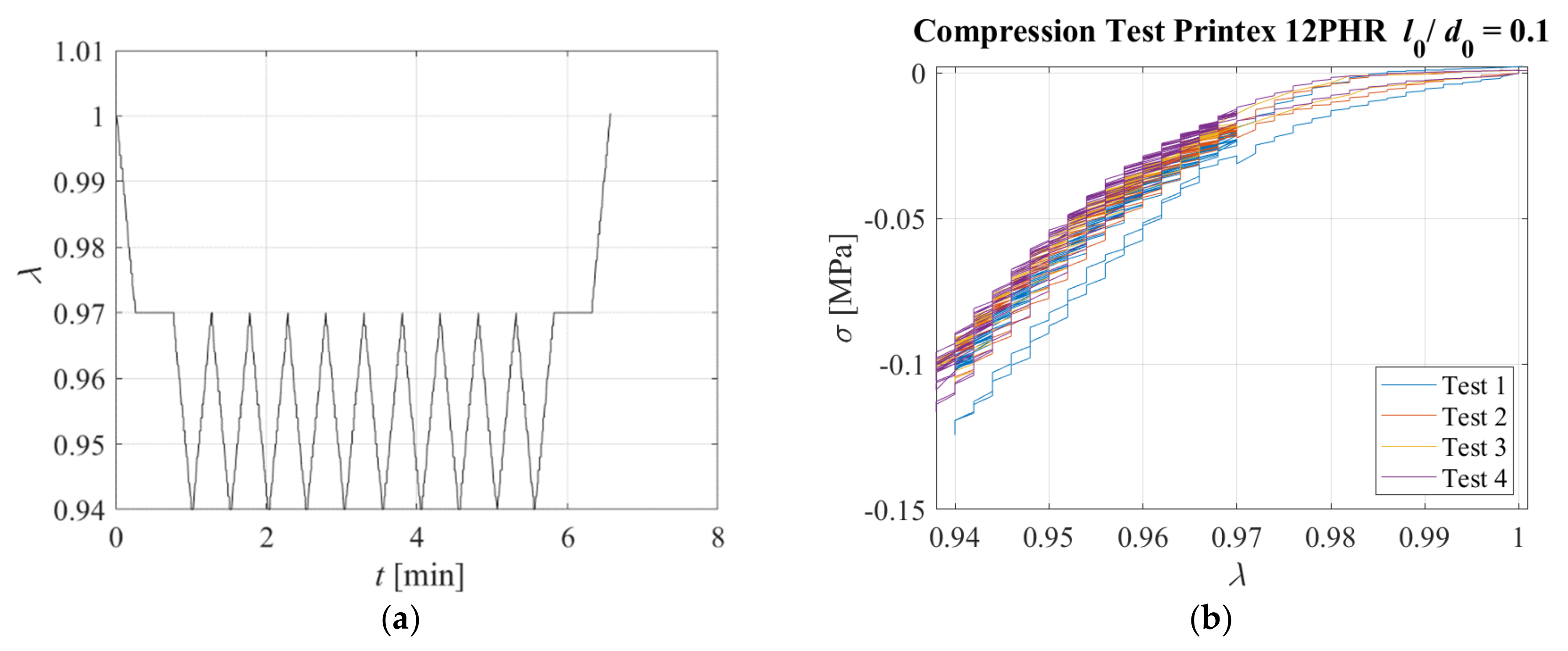
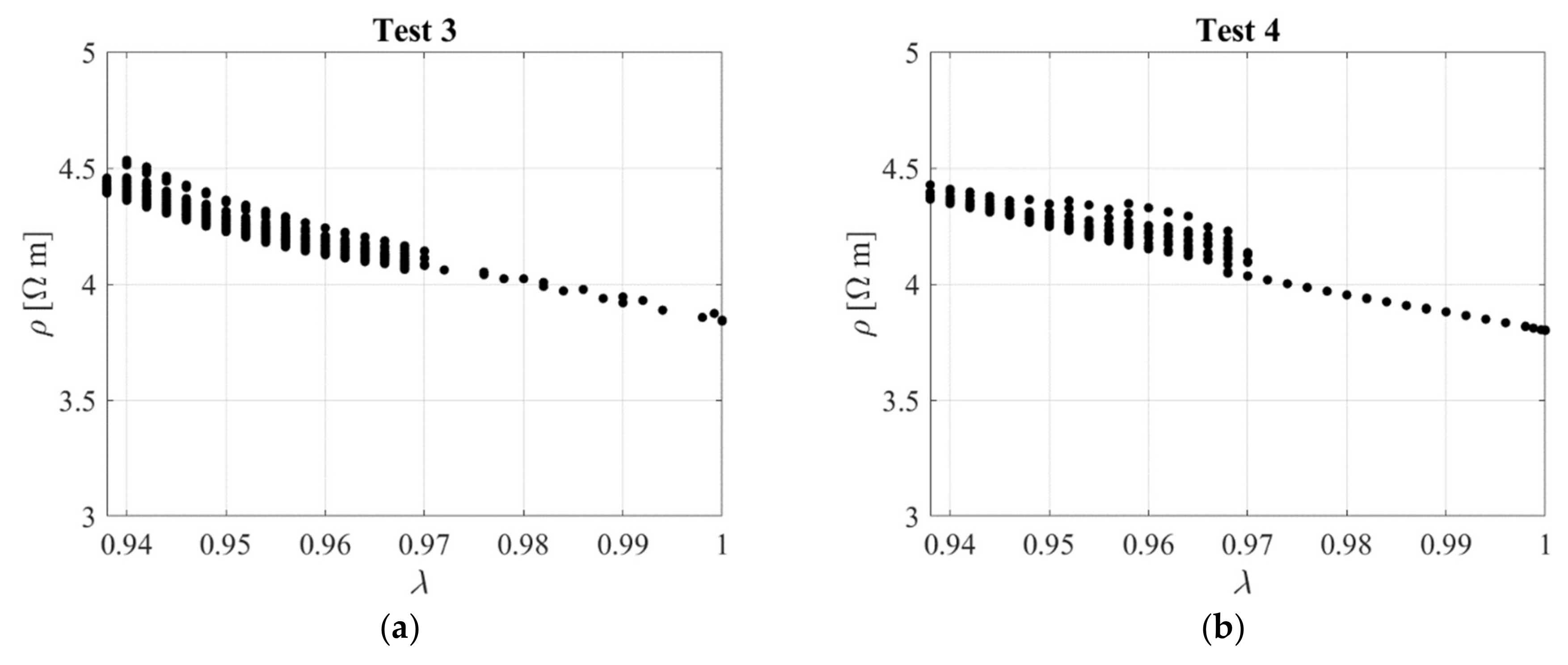
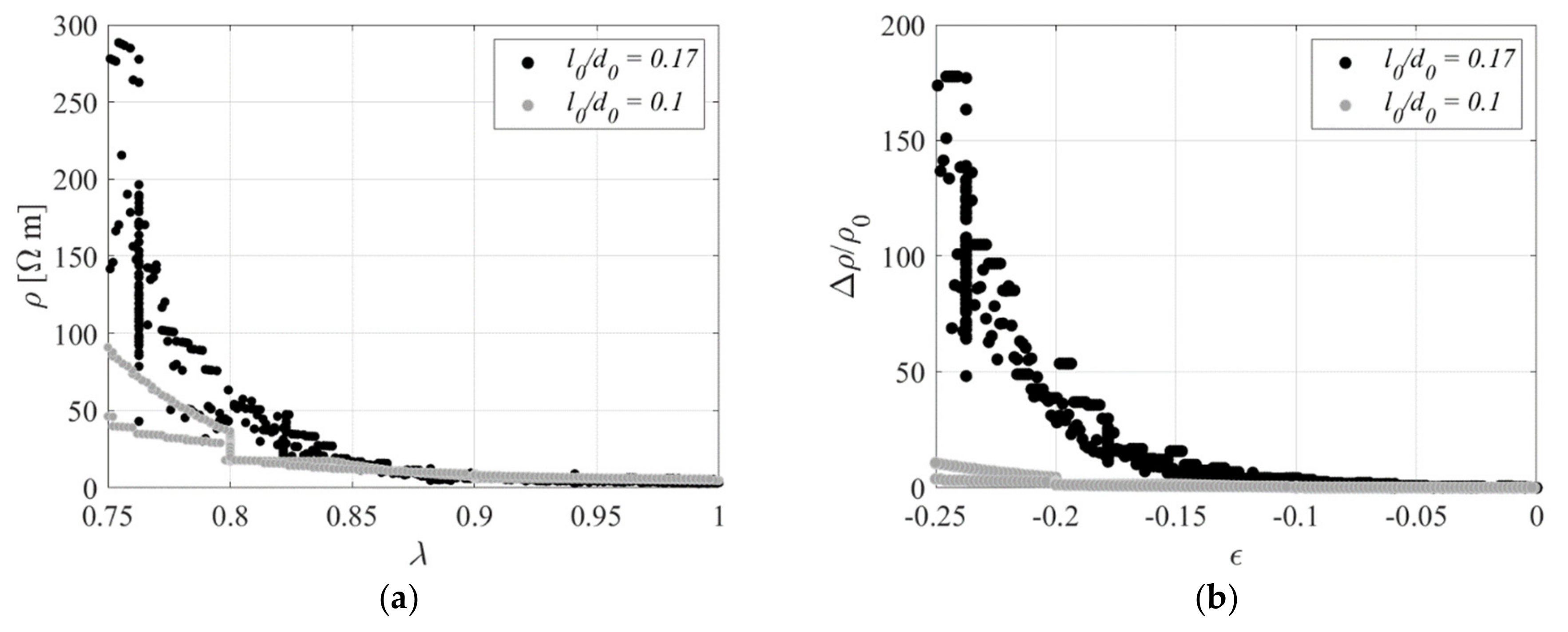
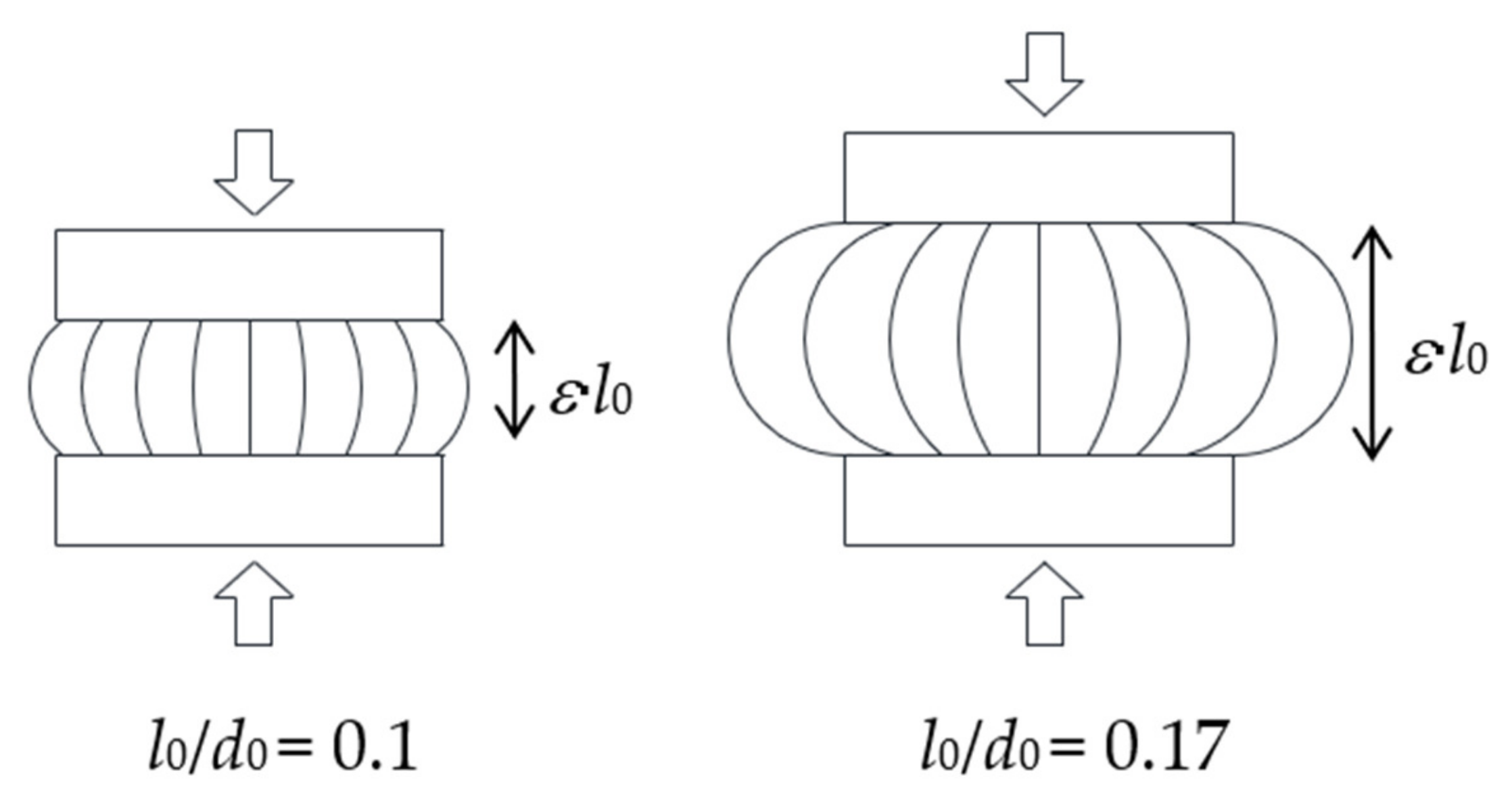
5.2. Compression Tests on Rubber Filled with Printex 12 Phr (Specimen with l0/d0 = 0.1)
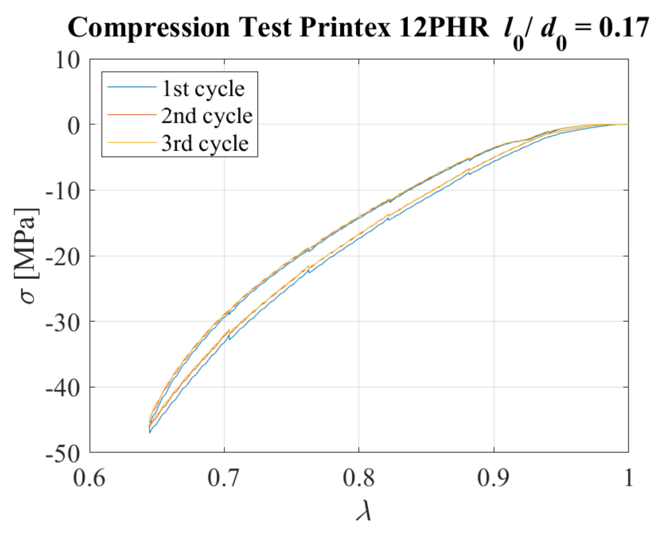
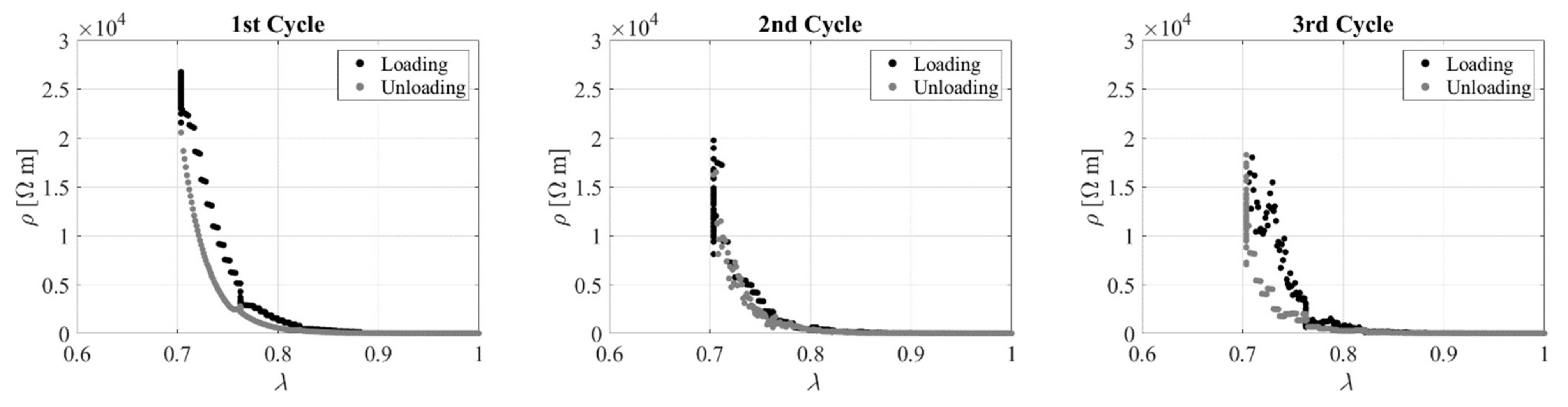
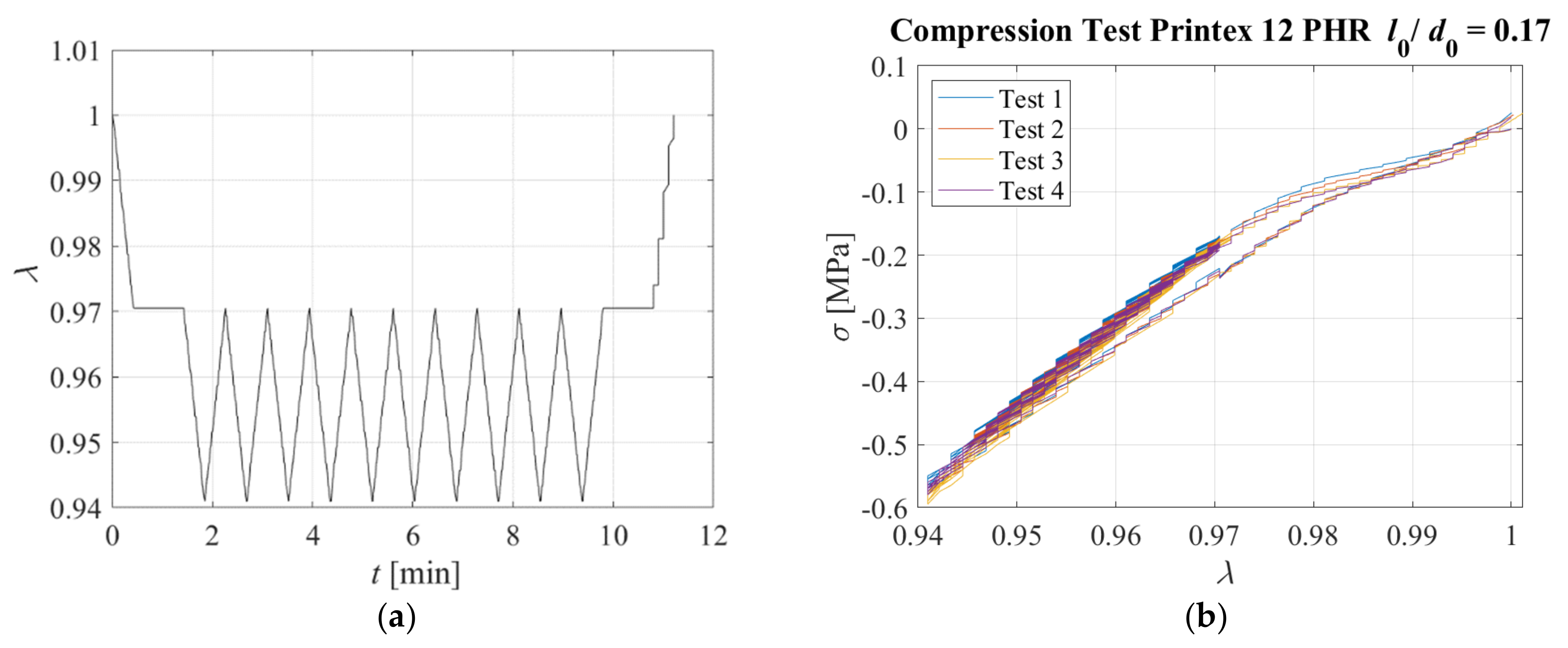
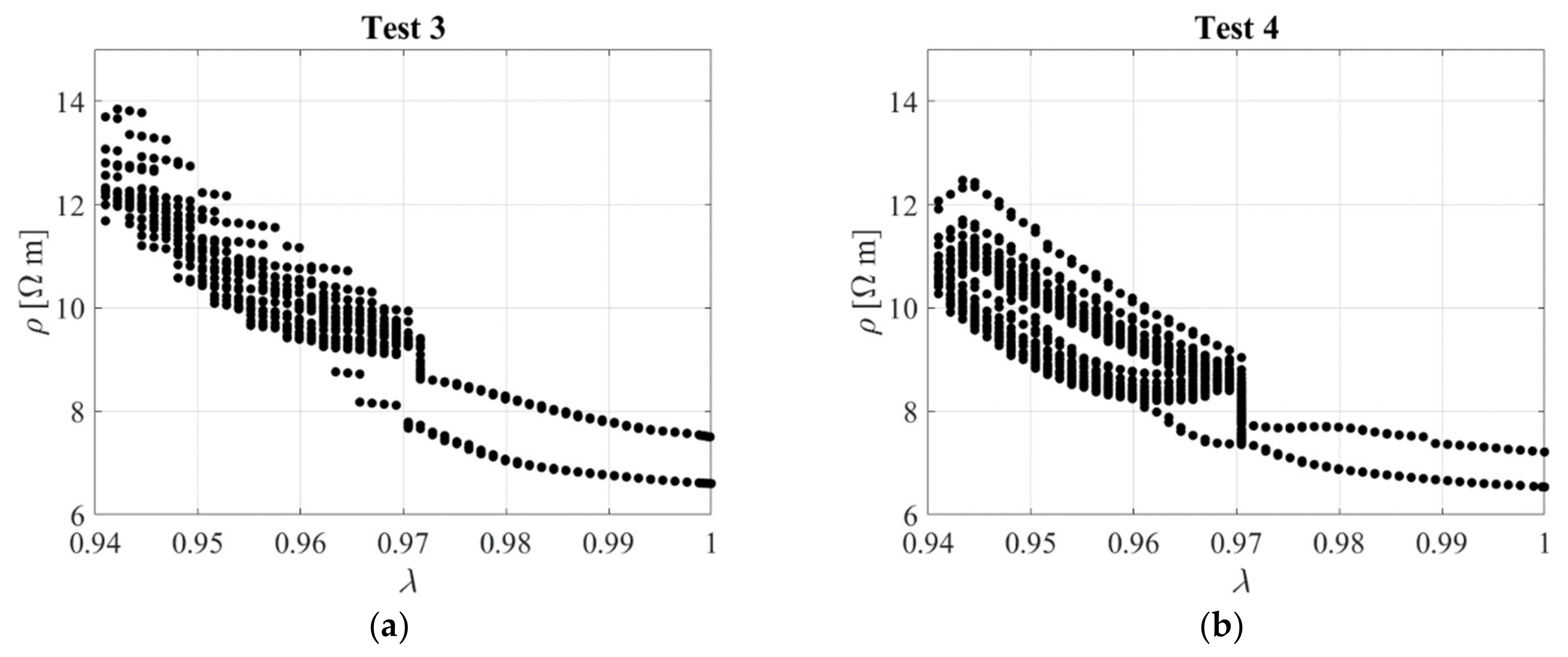
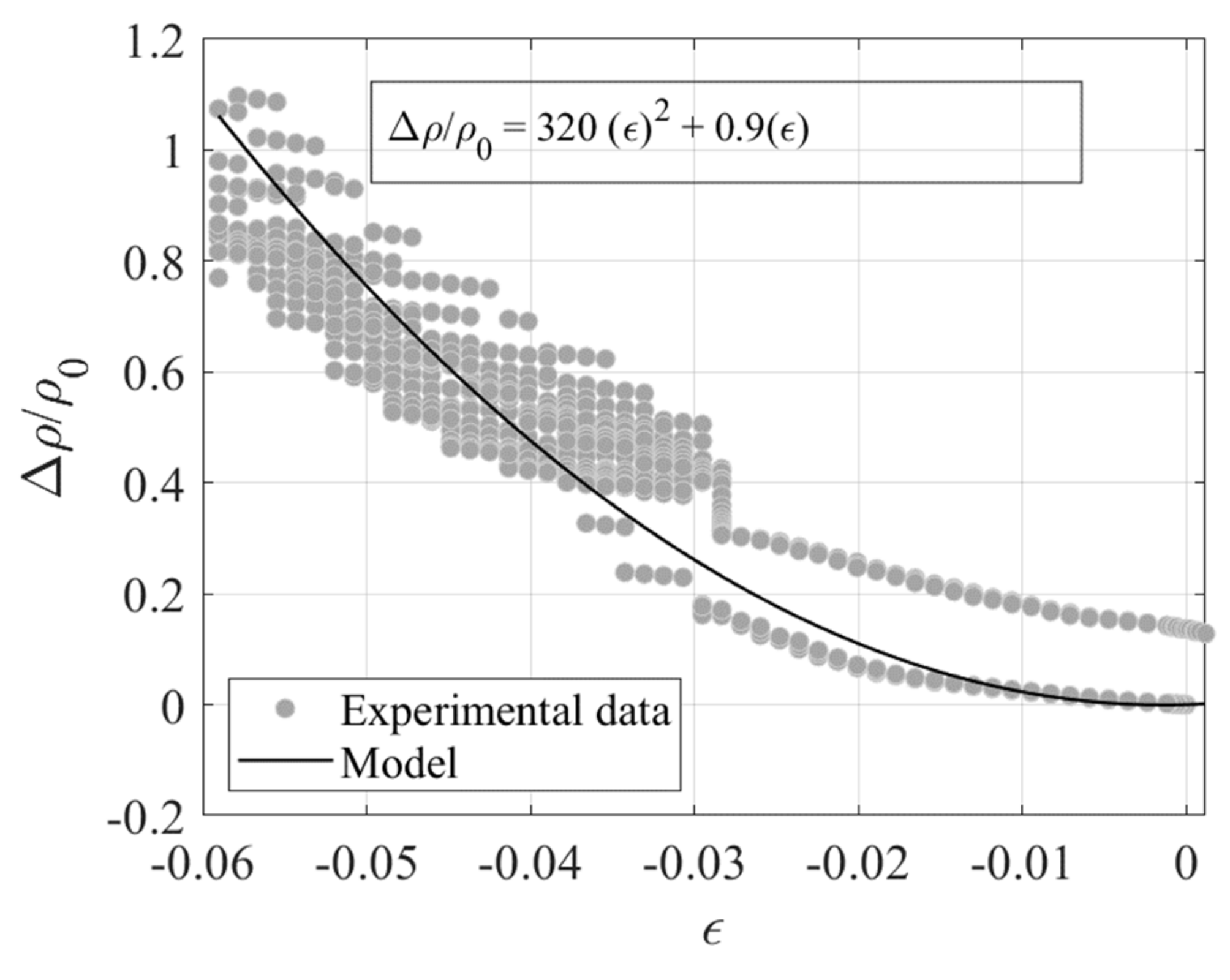
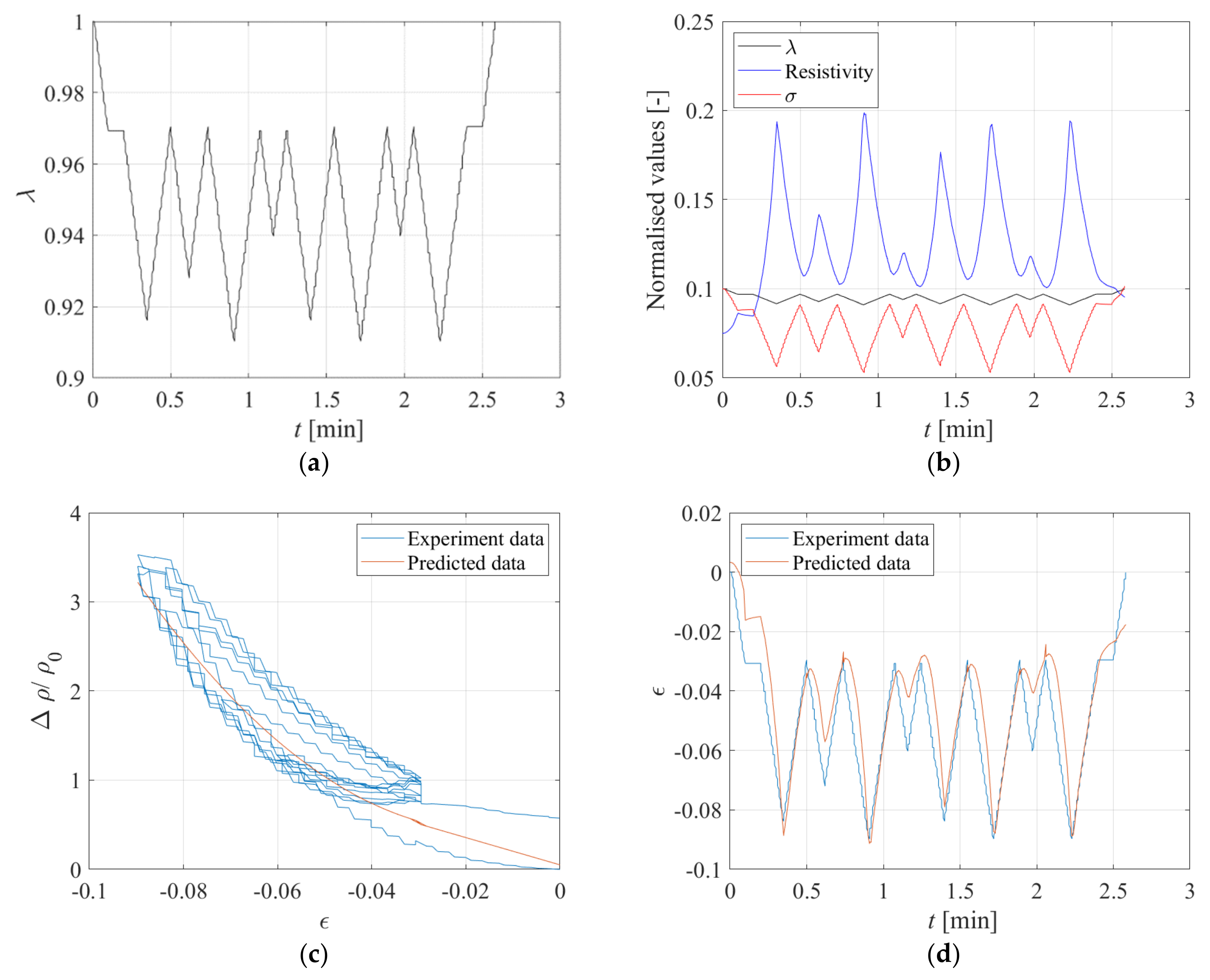
5.3. Compression Tests on Rubber Filled with Printex 12 Phr (Specimen with l0/d0= 0.17)
6. Summary and Discussion of Results
7. Conclusions and Future Studies
- —
- only the compounds filled with Printex XE2 have a significant potential for being used to develop smart rubber bearings, thanks to their reversible behaviour;
- —
- simplified models relating the change of resistivity to the changes of strain have been successfully used to infer the state of strain in the rubber under random loading scenarios based on electrical resistivity measurements;
- —
- the aspect ratio of the rubber layer significantly affects the piezoresistive behaviour under compressive loading. Finite element analyses (FEA) using a coupled electrical–mechanical model of the specimen should be carried out to confirm this.
Author Contributions
Funding
Data Availability Statement
Acknowledgments
Conflicts of Interest
References
- Lee, D.J. Bridge Bearings and Expansion Joints; CRC Press: Boca Raton, FL, USA, 1994. [Google Scholar]
- Aria, M.; Akbari, R. Inspection, condition evaluation and replacement of elastomeric bearings in road bridges. Struct. Infrastruct. Eng. 2013, 9, 918–934. [Google Scholar] [CrossRef]
- Talbot, J.P.; Hunt, H.E.M. Isolation of buildings from rail-tunnel vibration: A review. Build. Acoust. 2003, 10, 177–192. [Google Scholar] [CrossRef]
- Tubaldi, E.; Mitoulis, S.A.; Ahmadi, H.; Muhr, A. A parametric study on the axial behaviour of elastomeric isolators in multi-span bridges subjected to horizontal seismic excitations. Bull. Earthq. Eng. 2016, 14, 1285–1310. [Google Scholar] [CrossRef] [Green Version]
- Tubaldi, E.; Ragni, L.; Dall’Asta, A.; Ahmadi, H.; Muhr, A. Stress softening behaviour of HDNR bearings: Modelling and influence on the seismic response of isolated structures. Earthq. Eng. Struct. Dyn. 2017, 46, 2033–2054. [Google Scholar] [CrossRef]
- Kelly, J.; Konstantinidis, D. Mechanics of Rubber Bearings for Seismic and Vibration Isolation; John Wiley & Sons: Hoboken, NJ, USA, 2011. [Google Scholar] [CrossRef]
- Agrawal, A.K.; Subramaniam, K.V.; Pan, Y. Development of Smart Bridge Bearings System: A Feasibility Study, Report Number C-02-02, 2005. Available online: https://rosap.ntl.bts.gov/view/dot/16158 (accessed on 12 March 2022).
- Freire, L.M.; de Brito, J.; Correia, J.R. Inspection Survey of Support Bearings in Road Bridges. J. Perform. Constr. Facil. 2013, 29, 04014098. [Google Scholar] [CrossRef]
- Soleimani, S.A.; Konstantinidis, D.; Balomenos, G.P. Nondestructive assessment of elastomeric bridge bearings using 3D digital image correlation. J. Struct. Eng. 2022, 148, 04021233. [Google Scholar] [CrossRef]
- Topkaya, C.; Yura, J.A. Test Method For Determining The Shear Modulus Of Elastomeric Bearings. J. Struct. Eng. 2002, 128, 797–805. [Google Scholar] [CrossRef]
- Akbari, R.; Maalek, S. Evaluation of the Shear Modulus of Elastomeric Bridge Bearings Using Modal Data. J. Test. Eval. 2009, 37, 150–159. [Google Scholar]
- Li, S.; Ning, Q.; Chen, H. Rail Elevated Bridge Bearing Displacement Monitoring Based on FBG Sensor. Appl. Mech. Mater. 2012, 178, 2034–2037. [Google Scholar] [CrossRef]
- Liu, Q.; Li, G.; Jiang, R.; Yu, F.; Gai, W. An Intelligent Monitoring Method and Its Experiment for Bridge Bearing. In Proceedings of the 2016 International Conference on Civil, Transportation and Environment, Guangzhou, China, 30–31 January 2016; pp. 633–638. [Google Scholar]
- Kim, J.; Park, Y.; Choi, I.; Kang, D. Development of smart elastomeric bearing equipped with PVDF polymer film for monitoring vertical load through the support. VDI BERICHTE 2002, 1685, 135–140. [Google Scholar]
- Yamaguchi, K.; Busfield, J.J.C.; Thomas, A.G. Electrical and mechanical behavior of filled elastomers. I. The effect of strain. J. Polym. Sci. Part B Polym. Phys. 2003, 41, 2079–2089. [Google Scholar] [CrossRef]
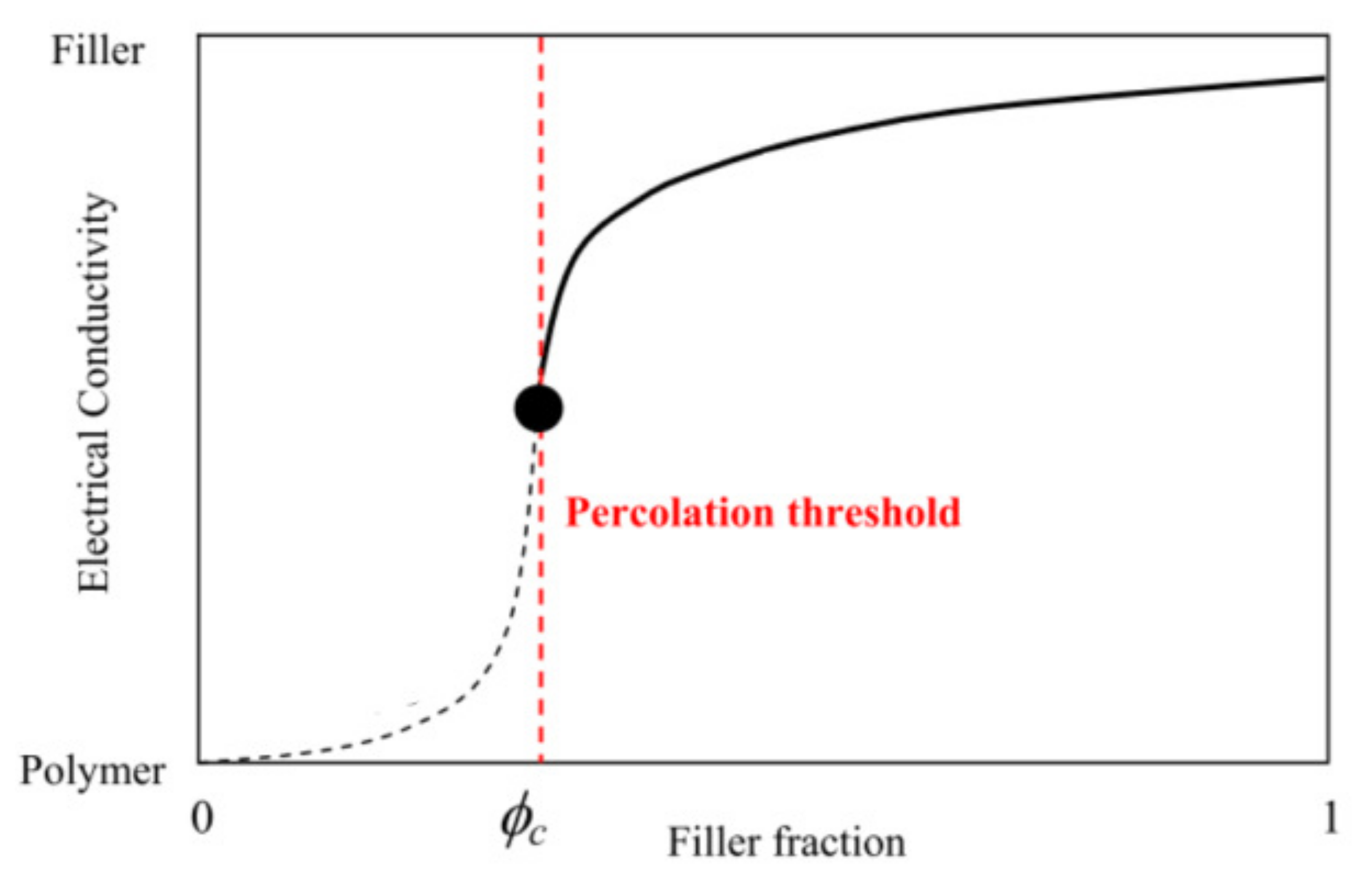
- Nan, C.W.; Shen, Y.; Ma, J. Physical properties of composites near percolation. Annu. Rev. Mater. Res. 2010, 40, 131–151. [Google Scholar] [CrossRef]
- Stauffer, D.; Aharony, A. Introduction to Percolation Theory, 2nd ed.; Taylor & Francis: Abingdon, UK, 1992. [Google Scholar] [CrossRef]
- Lim, A.S.; Melrose, Z.R.; Thostenson, E.T.; Chou, T.W. Damage sensing of adhesively-bonded hybrid composite/steel joints using carbon nanotubes. Compos. Sci. Technol. 2011, 71, 1183–1189. [Google Scholar] [CrossRef]
- Sam-Daliri, O.; Faller, L.M.; Farahani, M.; Roshanghias, A.; Araee, A.; Baniassadi, M.; Oberlercher, H.; Zangl, H. Impedance analysis for condition monitoring of single lap CNT-epoxy adhesive joint. Int. J. Adhes. Adhes. 2019, 88, 59–65. [Google Scholar] [CrossRef]
- Ahmed, S.; Thostenson, E.T.; Schumacher, T.; Doshi, S.M.; McConnell, J.R. Integration of carbon nanotube sensing skins and carbon fiber composites for monitoring and structural repair of fatigue cracked metal structures. Compos. Struct. 2018, 203, 182–192. [Google Scholar] [CrossRef]
- Sam-Daliri, O.; Faller, L.M.; Farahani, M.; Zangl, H. Structural health monitoring of adhesive joints under pure mode I loading using the electrical impedance measurement. Eng. Fract. Mech. 2021, 245, 107585. [Google Scholar] [CrossRef]
- Busfield, J.J.C.; Thomas, A.G.; Yamaguchi, K. Electrical and mechanical behavior of filled elastomers 2: The effect of swelling and temperature. J. Polym. Sci. Part B Polym. Phys. 2004, 42, 2161–2167. [Google Scholar] [CrossRef]
- Busfield, J.J.C.; Thomas, A.G.; Yamaguchi, K. Electrical and mechanical behavior of filled rubber. III. Dynamic loading and the rate of recovery. J. Polym. Sci. B Polym. Phys. 2005, 43, 1649–1661. [Google Scholar] [CrossRef]
- Jha, V.; Thomas, A.G.; Bennett, M.; Busfield, J.J.C. Reversible Electrical Behavior with Strain for a Carbon Black-Filled Rubber. J. Appl. Polym. Sci. 2010, 116, 2658–2667. [Google Scholar] [CrossRef]
- Giannone, P.; Graziani, S.; Umana, E. Investigation of carbon black loaded natural rubber piezoresistivity. In Proceedings of the 2015 IEEE International Instrumentation and Measurement Technology Conference (I2MTC) Proceedings, Pisa, Italy, 11–14 May 2015; pp. 1477–1481. [Google Scholar]
- Nims, D.K.; Subramaniam, K.; Parvin, A.; Aktan, A.E. The Potential for the Use of Elastomeric Bearings in an Intelligent Bridge System. In Proceedings of the Transportation Research Board 75th Annual Meeting, Washington, DC, USA, 8–10 January 1996. [Google Scholar]
- Nims, D.K. Instrumented Elastomeric Bridge Bearings; ODOT Project No. 14647(0), Final Report; University of Toledo: Toledo, OH, USA, 2000. [Google Scholar]
- Subramaniam, K.V. Feasibility of Using Instrumented Elastomeric Bearings for Bridge Monitoring and Condition Assessment. Master’s Thesis, University of Toledo, Toledo, OH, USA, 1995. [Google Scholar]
- Moses, F. Weigh-in-motion system using instrumented bridges. Transp. Eng. J. ASCE 1979, 105, 233–249. [Google Scholar] [CrossRef]
- OBrien, E.J.; Enright, B.; Getachew, A. Importance of the tail in truck weight modeling for bridge assessment. J. Bridge Eng. 2010, 15, 210–213. [Google Scholar] [CrossRef]
- Sae-Oui, P.; Thepsuwan, U.; Thaptong, P.; Sirisinha, C. Comparison of reinforcing efficiency of carbon black, conductive carbon black, and carbon nanotube in natural rubber. Adv. Polym. Technol. 2014, 33. [Google Scholar] [CrossRef]
- McAlorum, J.; Perry, M.; Ward, A.C.; Vlachakis, C. ConcrEITS: An Electrical Impedance Interrogator for Concrete Damage Detection Using Self-Sensing Repairs. Sensors 2021, 21, 7081. [Google Scholar] [CrossRef] [PubMed]
- Kingston, J.G.R.; Muhr, A.H. Effect of scragging on parameters in viscoplastic model for filled rubber. Plast. Rubber Compos. 2011, 40, 161–168. [Google Scholar] [CrossRef]
- AASHTO. LRFD Bridge Design Specifications; American Association of State Highway and Transportation Officials: Washington, DC, USA, 2008. [Google Scholar]


| Material | Abbreviation | ||
|---|---|---|---|
| Standard Malaysian Rubber | SMR | ||
| High abrasion furnace | HAF | ||
| Hexyl phenyl phenylenediamine | HPPD | ||
| Cyclohezyl benzothiazxy sulphenamide | CBS | ||
| Tertiary butyl benzothiazole sulfenamide | TBBS | ||
| Ingredients | Parts per hundred of rubber (phr) | ||
| carbon black 70 phr | Printex XE2 15 phr | Printex XE2 12 phr | |
| NR (SMR CV60) | 100 | 100 | 100 |
| Carbon black (N330 HAF) | 70 | - | - |
| Printex XE2 | - | 15 | 12 |
| Stearic acid | 2 | 2 | 2 |
| Zinc oxide | 10 | 7 | 7 |
| Antioxidant (HPPD) | 1 | - | - |
| Cobalt naphthenate | 3 | - | - |
| Accelerator (CBS) | 0.8 | - | - |
| 6PPD | - | 1.5 | 1.5 |
| Antilux 654 | - | 1.5 | 1.5 |
| Manobond 740 C | - | 0.75 | 0.75 |
| TBBS | - | 1.5 | 1.5 |
| Sulphur | 4 | 1.5 | 1.5 |
| Test Pieces | Loading | ||||
|---|---|---|---|---|---|
| Tensile | Shear | Compression | |||
| Full Cycle | Triangular | Random | |||
| Carbon black tensile specimen | ✓ | ✓ | |||
| Printex 15 phr tensile specimen | ✓ | ✓ | |||
| Printex 12 phr Double Bonded Shear (DBS) specimen | ✓ | ||||
| Printex 12 phr compressive disc specimen l0/d0 = 0.1 | ✓ | ||||
| Printex 12 phr compressive disc specimen l0/d0 = 0.17 | ✓ | ||||
| Test 1 | Test 2 | Test 3 | Test 4 | |
|---|---|---|---|---|
| λ [-] | 1.3 | 1.4 | 1.6 | 2 |
| [s−1] | 0.05 | 0.1 | 0.05 | 0.05 |
| Test 1 | Test 2 | Test 3 | Test 4 | |
|---|---|---|---|---|
| [s−1] | 0.0017 | 0.0017 | 0.0075 | 0.0075 |
| [s−1] | 0.0017 | 0.0017 | 0.0017 | 0.01 |
| Dwell time [s] | 30 | 6 | 6 | 3 |
| Test 1 | Test 2 | Test 3 | Test 4 | |
|---|---|---|---|---|
| [s−1] | 0.0017 | 0.0017 | 0.0075 | 0.0075 |
| [s−1] | 0.0017 | 0.0017 | 0.0017 | 0.01 |
| Dwell time [s] | 30 | 6 | 6 | 3 |
| Specimens | GF | σε |
|---|---|---|
| Printex 15 phr tensile specimen | 9.27 | 0.16 |
| Printex 12 phr compressive specimen l0/d0 = 0.1 (SF = 2.5) | 2.10 | 0.005 |
| Printex 12 phr compressive specimen l0/d0 = 0.17 (SF = 5.88) | 11.5 | 0.0085 |
Disclaimer/Publisher’s Note: The statements, opinions and data contained in all publications are solely those of the individual author(s) and contributor(s) and not of MDPI and/or the editor(s). MDPI and/or the editor(s) disclaim responsibility for any injury to people or property resulting from any ideas, methods, instructions or products referred to in the content. |
© 2023 by the authors. Licensee MDPI, Basel, Switzerland. This article is an open access article distributed under the terms and conditions of the Creative Commons Attribution (CC BY) license (https://creativecommons.org/licenses/by/4.0/).
Share and Cite
Orfeo, A.; Tubaldi, E.; McAlorum, J.; Perry, M.; Ahmadi, H.; McDonald, H. Self-Sensing Rubber for Bridge Bearing Monitoring. Sensors 2023, 23, 3150. https://doi.org/10.3390/s23063150
Orfeo A, Tubaldi E, McAlorum J, Perry M, Ahmadi H, McDonald H. Self-Sensing Rubber for Bridge Bearing Monitoring. Sensors. 2023; 23(6):3150. https://doi.org/10.3390/s23063150
Chicago/Turabian StyleOrfeo, Alessandra, Enrico Tubaldi, Jack McAlorum, Marcus Perry, Hamid Ahmadi, and Hazel McDonald. 2023. "Self-Sensing Rubber for Bridge Bearing Monitoring" Sensors 23, no. 6: 3150. https://doi.org/10.3390/s23063150