
A Pipe-Embeddable Impedance Sensor for Monitoring Water Leaks in Distribution Networks: Design and Validation

Abstract
:1. Introduction
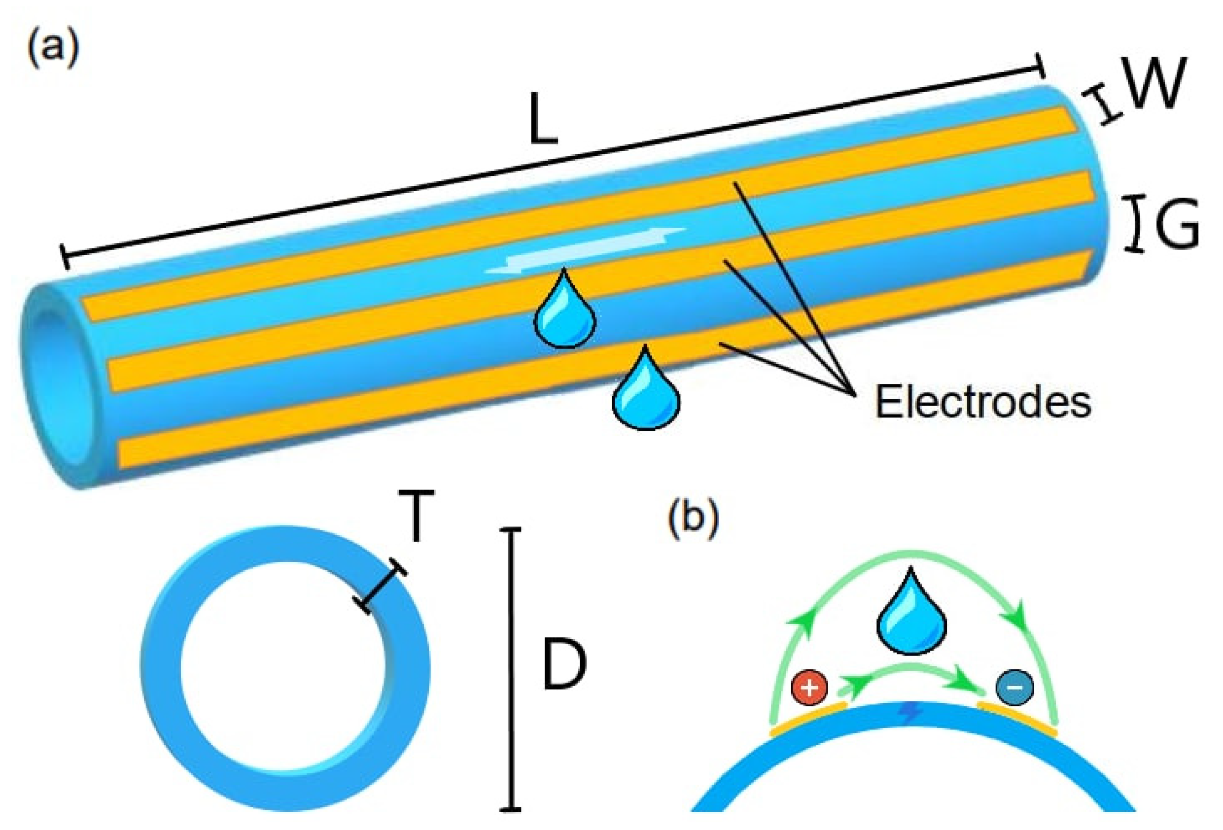
2. Simulations
2.1. Enhanced Model
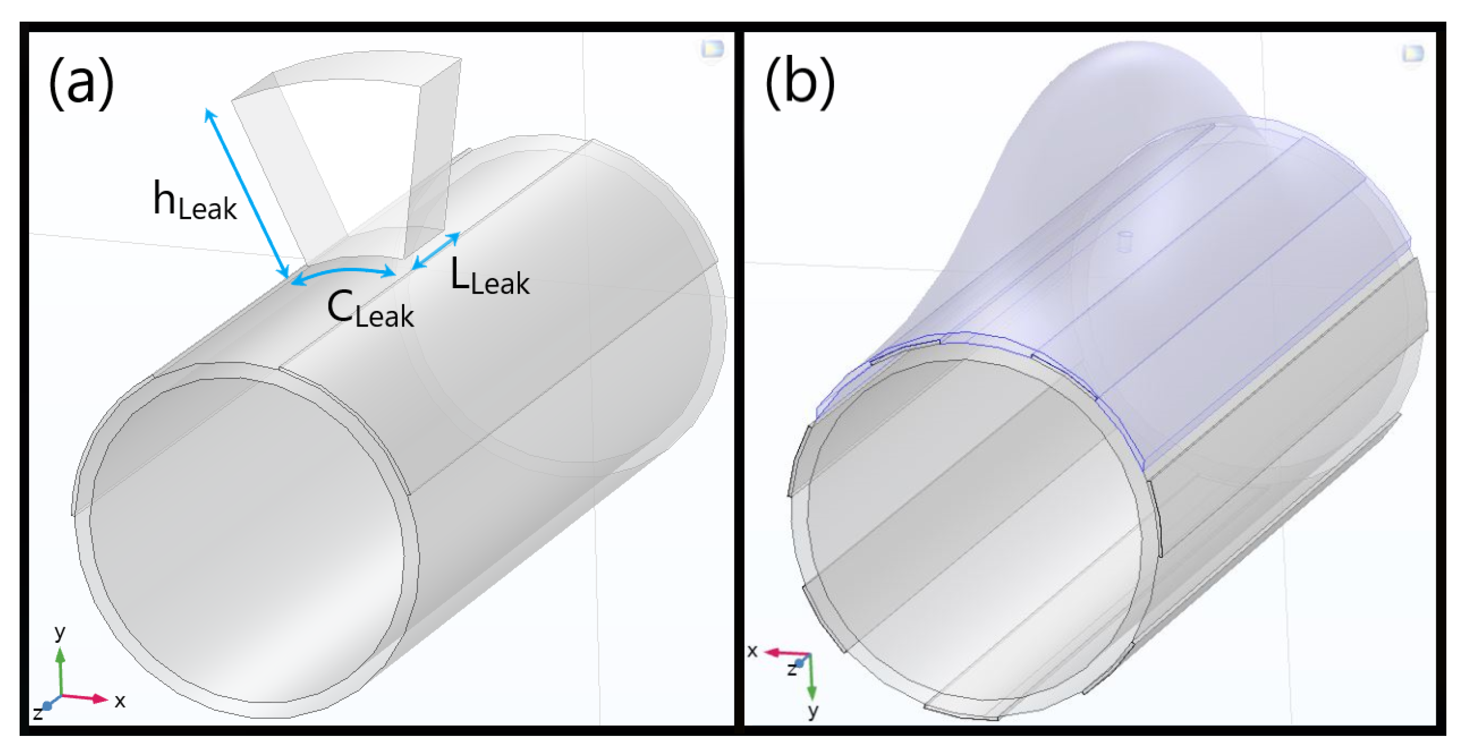
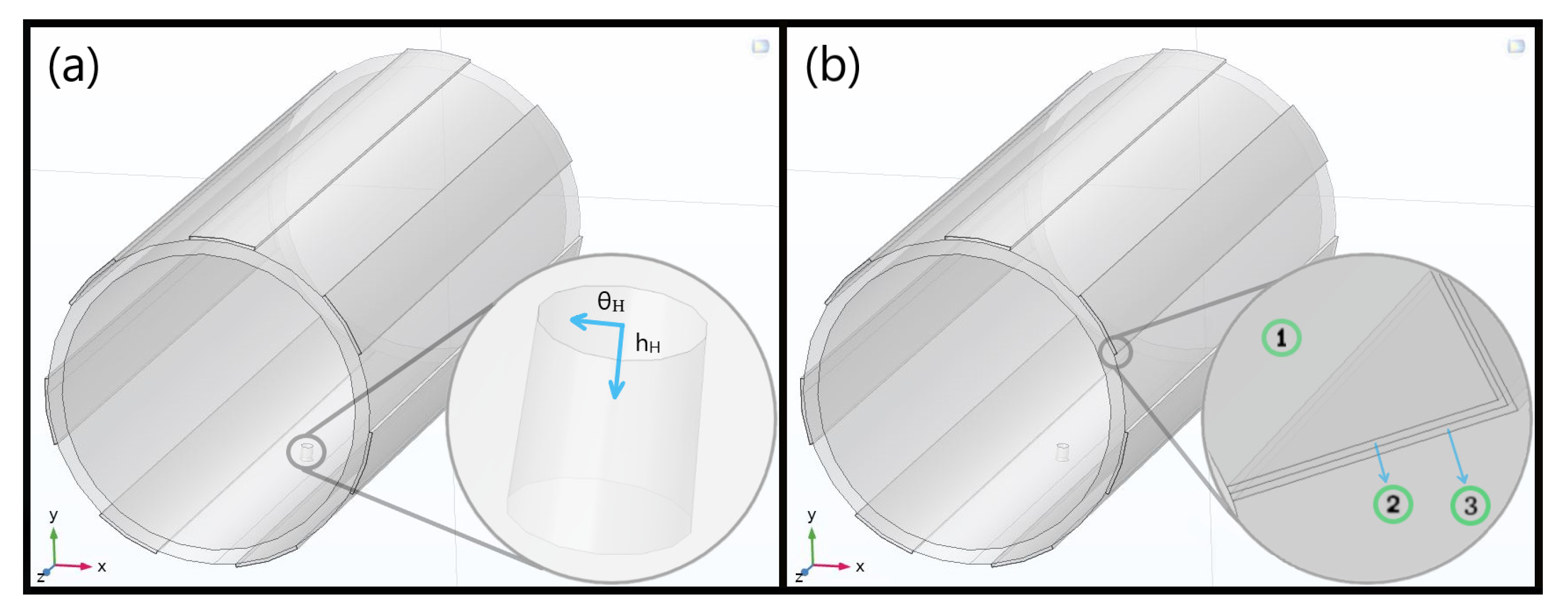
2.2. Leakage Spatial Detectability
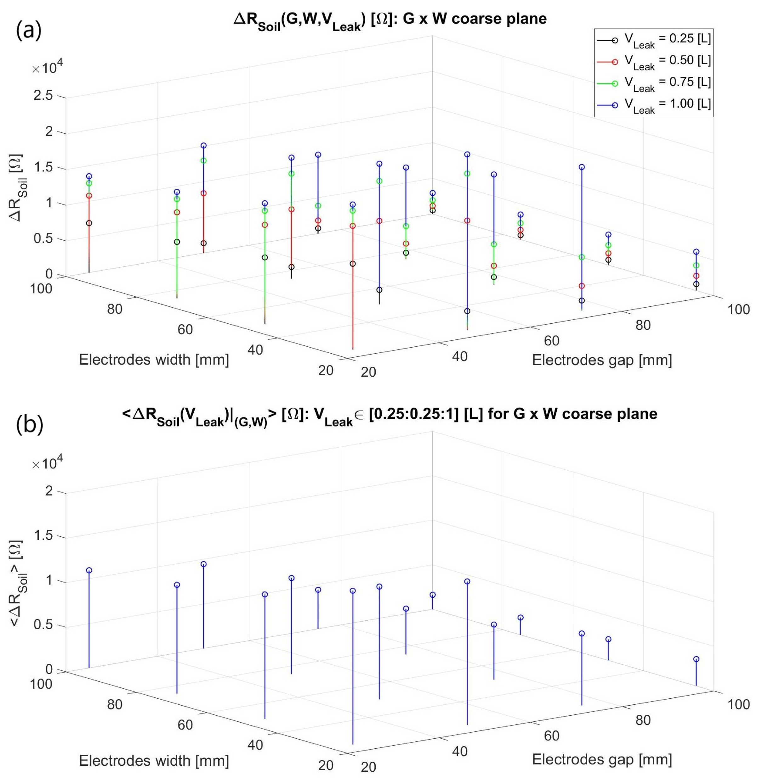
2.3. Electrodes Size Optimization
3. Experimental Results
3.1. Preliminary Measurements
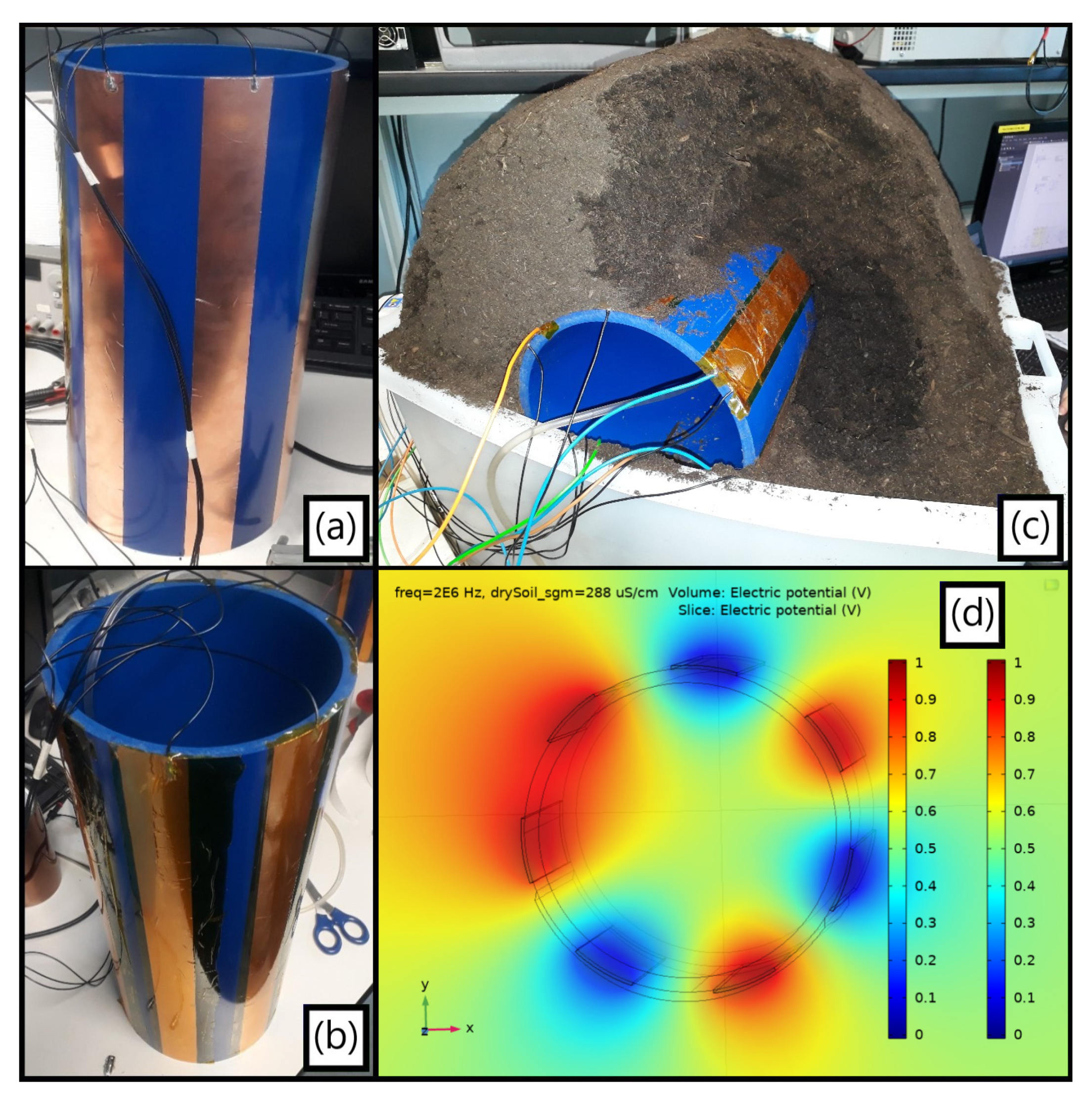
3.1.1. Single Electrode Pair
- (1)
- Exposed electrodes outcomes: The outer air environment is sensed by the non-insulated metal strips as an almost ideal capacitance from the intermediate frequency range onwards due to its poor electrical conductivity. On the other hand, the water ionic composition leads to a quasi-resistive comportment. The entrance capacitive element CKp introduced by the polyimide coverage has an impact of up to 1 MHz when comparing the two aqueous scenarios, above which the impedance converges to the RH20 resistive plateau in both cases. Finally, no exposed copper electrodes test with an encircling dry soil was performed hitherto because it would not consist of the final target design.
- (2)
- Insulation issue: The shortening process for the CKp element in the dry soil scenario can be verified at the yellow phase plot curve at around the same frequency order of magnitude as in the aqueous one. However, its inferior ∂(ΦSoil)/∂f leads to a lower phase peaking and implies that RSoil tends to vanish within |Z(jω)| due to the proximity between the CKp zero singularity and a preexistent higher-frequency pole related to CSoil and RSoil. Although imposing a readout frequency (fR) above the original 1 kHz was a foreseen requirement due to the CKp’s existence along with a real ground conductivity diminishing the predicted RSoil from being about one hundred times superior to the initially surmised 1 µS/cm as later estimated, a complementary alternative had to be devised for trying to reduce the aforesaid zero so as to still enable tracking of the RSoil plateau.
- (3)
- Insulation alternative: The sensor width was doubled from 20 to 40 mm as an endeavor to reduce fR by enlarging CKp and empirically derive such a widening impact departing from the originally quasi-optimal 2 cm dimension. As can be ascertained in Figure 7, not only did the CKp increase but also RSoil diminished, since the former depends linearly at a first order on the electrodes’ area whereas the latter does so hyperbolically. Nonetheless, both their intricate relation with the residual geometrical parameters and the electric field spatial distribution still culminated in a slight alteration at the zero singularity.
3.1.2. Effect of Soil Thickness
- (1)
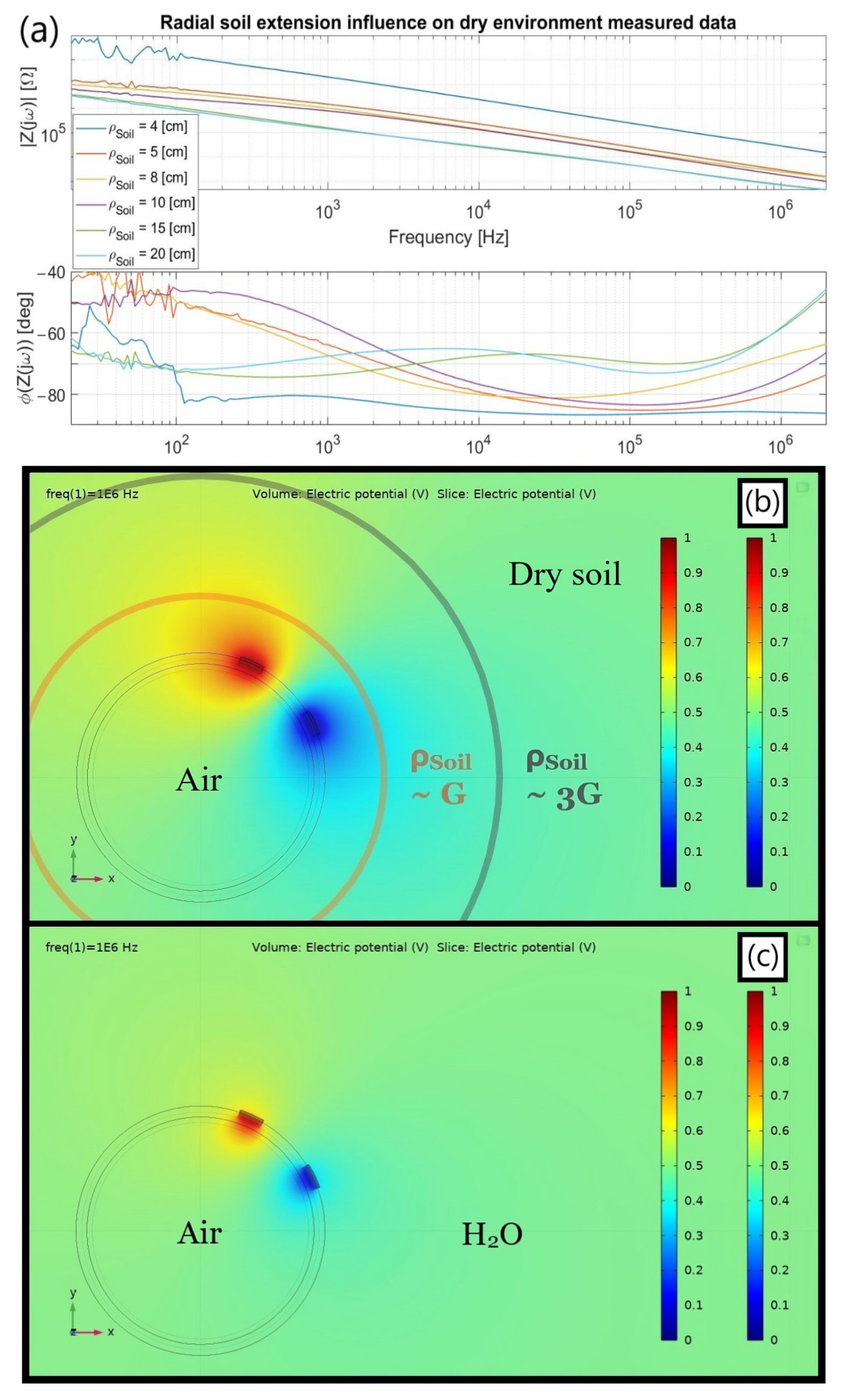
- Environmental elements disguise: For the lowest ρSoil, the CSoil and RSoil parallel connection seems to become virtually huge to the point that the inner capacitive branch formed by the series of CPipe and CAir tends to dominate the outer vs. inner current dispute. As inspected in Figure 9a, an essentially steady −90° phase is achieved apart from the initially bouncy values, presumably due to a large RAir soon shortened by CAir, hence setting an internal capacitive coupling behavior. As ρSoil increases, such an inner dominance seems to be overtaken by the outer branch since RSoil decreases and CSoil enlarges to their expected values for an “infinite” outer medium radius, a priori being ρSoil > 3 G. Consequently, the greater ρSoil, the smaller the inner capacitive effect and the easier the RSoil measurability.
- (2)
- Prototype correction: Besides ρSoil, the ongoing geometrical dependence also has a non-negligible influence even for the lateral plastic walls holding the soil altogether. Although not hereby shown for the sake of simplicity, positioning the tube longitudinal axis parallel to the shorter or longer box sides slightly influences the outcomes, the former having more consistent results since a larger terrain amount radially enfolds the electrodes.
- (3)
- CKp vs. Constant Phase Element (CPE): the intermediate and low frequency ranges in Figure 9a were not focused due to some intrinsic non-linearities beyond the simplified proposed circuit scope. For instance, there is a zero-pole cancellation tendency at intermediate frequencies that evolves to a CPE demeanor in the interdigitated structure when both impose correct ρSoil values. As will be shown, the latter replaces CKp in a refined equivalent model and exists primarily due to a thin ionic double layer formed on top of the polyimide tape that affects not only the access capacitance but also the local conductivity around it.
3.2. Interdigitated Structure
3.2.1. Single-Ended Leakage Detection
3.2.2. Electrical Parameters
- (1)
- Initial double layer and Kapton®: The same (σdL,Kp)dry conductivity was used for both equally sized layers in a dry terrain scenario and for electrodes not affected by the leak, strongly influencing the spectra below 1 kHz. However, the obtained double layer permittivity of (εr,dL)dry = 0.35 is not feasible since an even tinier one would be achieved for its nanometric real thickness, this being the main reason to impose a thicker soil when seeking for a better consistency. As for the local conductivity around their insulating material, it increases when electrodes are directly covered by wet soil, a fact impacting the low-frequency range and modelled through a higher double layer conductivity for the two strips covered by the leakage. Similarly, the water dissemination introduces a wider ionic concentration into the terrain, overcoming that of an arid soil, hence rising the local (εr,dL)wet for the metal strips sensing it and diminishing the magnitude plot at [10, 100] kHz due to a smaller |1/jωCeq|, with Ceq−1 = CKp−1 + CdL−1. Nonetheless, as occurred for (εr,dL)dry, the best-fit cases once more converged to a physically incoherent value lower than the unit;
- (2)
- Unified ionic double layer and Kapton® (CPE//Req): For simulating a CPE in the F.E.M. environment, an imaginary relative permittivity was imposed for the unified insulating layer, with (εdL+Kp)dry = α εKp (jω)−0.17, α ∊ ℝ, and εKp = 3. Such an expression did properly satisfy both the achieved phase at the spectra intermediate ranges and the magnitude-frequency-dependent slope. Intriguingly, the CPE permittivity module |εr,CPE| also impinges on the ΔRSoil variation above 1 MHz through the α factor instead of solely in the region at which a regular capacitive entrance element should dominate. Hence, (σGnd)wet was not adequately pinpointed as in the antecedent numerical outcomes so that only an estimate is exhibited for the latter. Finally, the polyimide finite resistance dominates the equivalent one (Req) and mostly impacts the low-frequency range, (σdL+Kp)dry being one order of magnitude smaller than in the incorrect setup and increasing anew in the presence of water.
- (3)
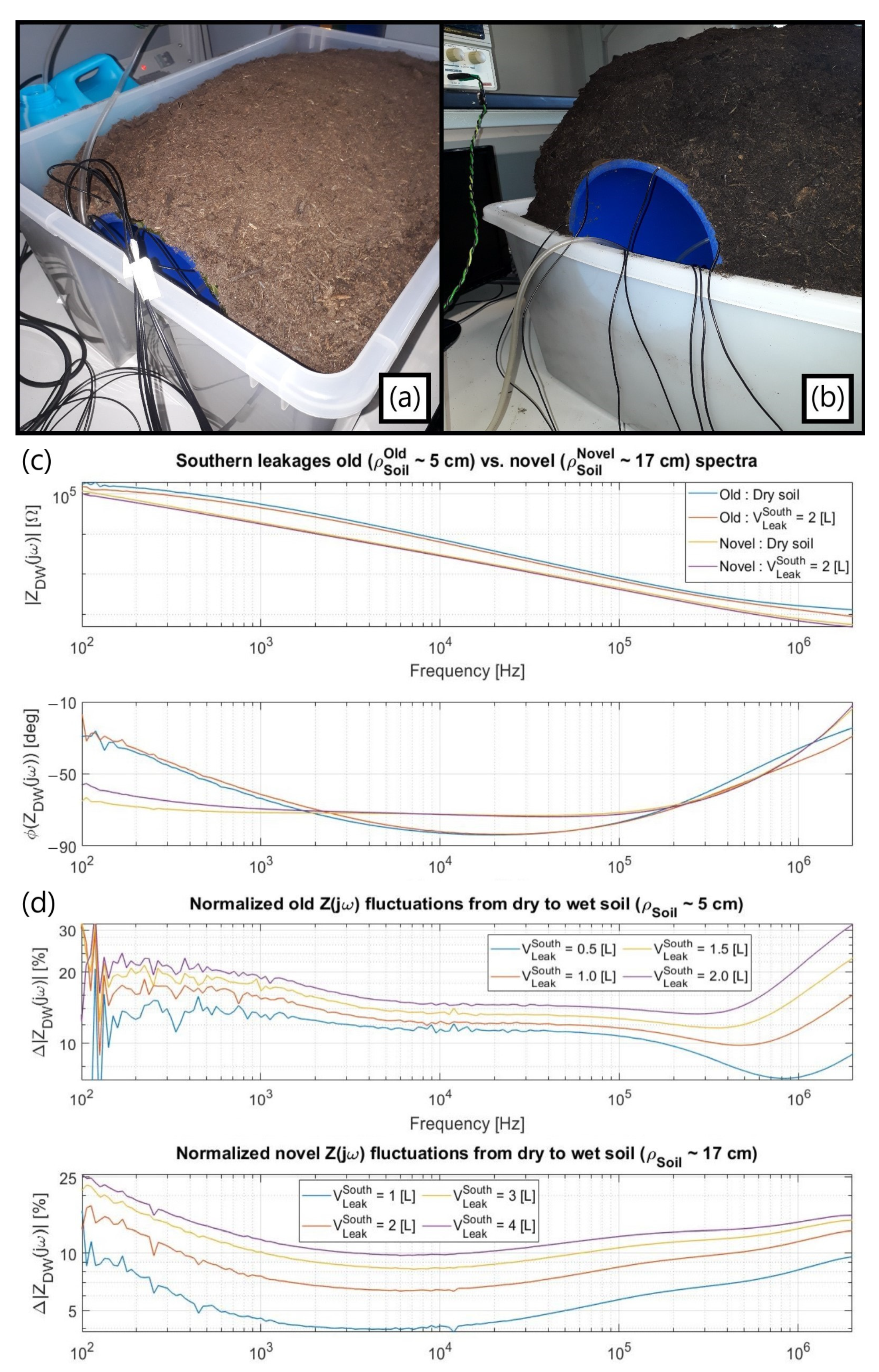
- Surrounding terrain and confined leak zone: The dry terrain conductivity (σGnd)dry impacts the spectra above 1 MHz and the zero singularity preceding the RSoil plateau. Its permittivity directly influences the pole after the RSoil zone, affecting mainly the verified phase around 1 MHz (LCR instrument limits the real detection up to 2 MHz). As for the wet terrain, increasing the confined 2 L Gaussian-alike infiltration conductivity indeed reduces the RSoil plateau as foreseen. Regarding its permittivity, a higher CSoil is attained when wet since εr,H2O > εr,Gnd, so once RSoil has been shortened by CSoil at frequencies above the LCR bandwidth, a shrinkage in the magnitude spectrum ultimately occurs as a result.
3.2.3. Refined Equivalent Circuit
- (1)
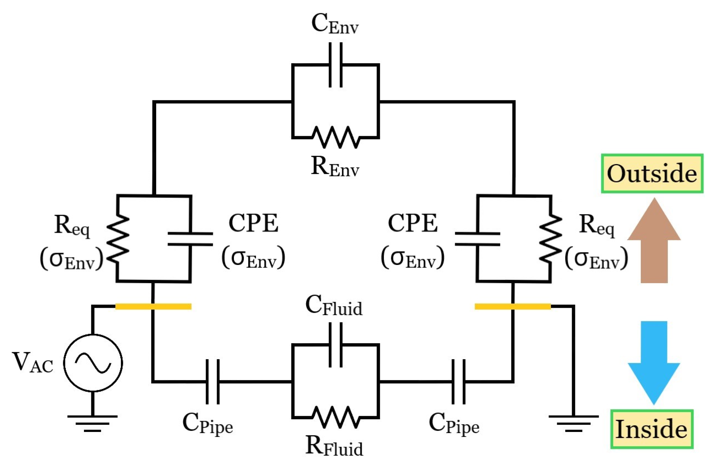
- Outer air environment: Due to the air’s poor electrical conductivity and permittivity, considerably large RAir and CAir are obtained for this external vicinity. As a result, given that Req also has a high impedance derived from the non-ideal insulating material, a reduced associated pole is predicted to occur so that an outer capacitive coupling is already reached from low frequencies. A similar coupling occurs in principle at the inner branch when air fills the conduit due to its tiny respective pole, presenting then a balanced impedance with respect to the outside. Conversely, a water filling is foreseen to entail a tendency for the internal impedance path to dominate the outer vs. inner parallel connection and ultimately reduce |Z(jω)| compared to the “empty” condition since RH2O << RAir and CH2O >> CAir. Moreover, the inner branch pole would be pushed forward in the spectrum (εH2O/σH2O << εAir/σAir), possibly culminating in a potentially trackable RH2O high-frequency plateau.
- (2)
- Outer soil environment (shallow terrain): As advocated for in Section 3.1.2, the electric field between the metal strips seems to be unavoidably compressed to a narrower transversal area if a proper amount of soil surrounding the pipe is not imposed, therefore virtually increasing RSoil and reducing CSoil so that a considerable part of the |Z(jω)| spectrum is lifted up. As a result, the CPE effect attained for the single-ended interdigitated scheme is reduced to an almost ideal capacitive demeanor at the intermediate spectra range. Nonetheless, the impedance related to the entrance capacitance region is still reduced from the water leak impact on the double layer, i.e., Ceq−1 = CKp−1 + CdL−1 decreases due to a greater CdL.
- (3)
- Outer soil environment (thick terrain): Apart from ensuring more accurate results, the corrected RSoil and CSoil could be potentially jeopardized in terms of the leak detection by the inner branch when moving from air to water filling since the internal path could potentially compete with the outer branch for the electrodes’ current and compromise the measurement. However, some empirical outcomes performed for the pipe filled with water and surrounded by soil still endorsed the leakage-sensing feasibility. A viable explanation is that the inner water-related pole is likely pushed forward beyond the LCR meter limit of 2 MHz resolution, hence not compromising the Δ|Z(jω)| variation at the RSoil spectrum region.
3.3. Non-Ideal Effects
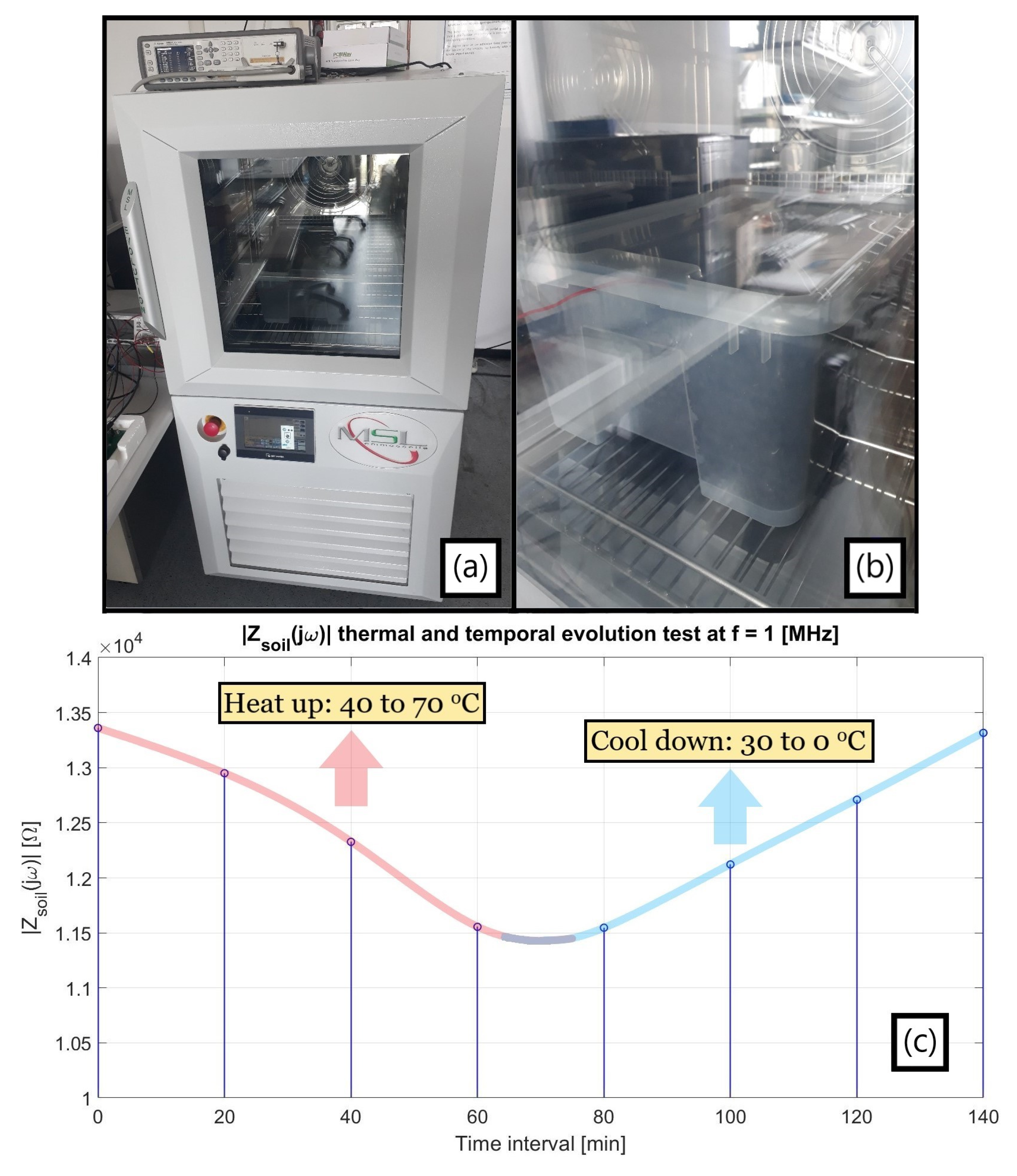
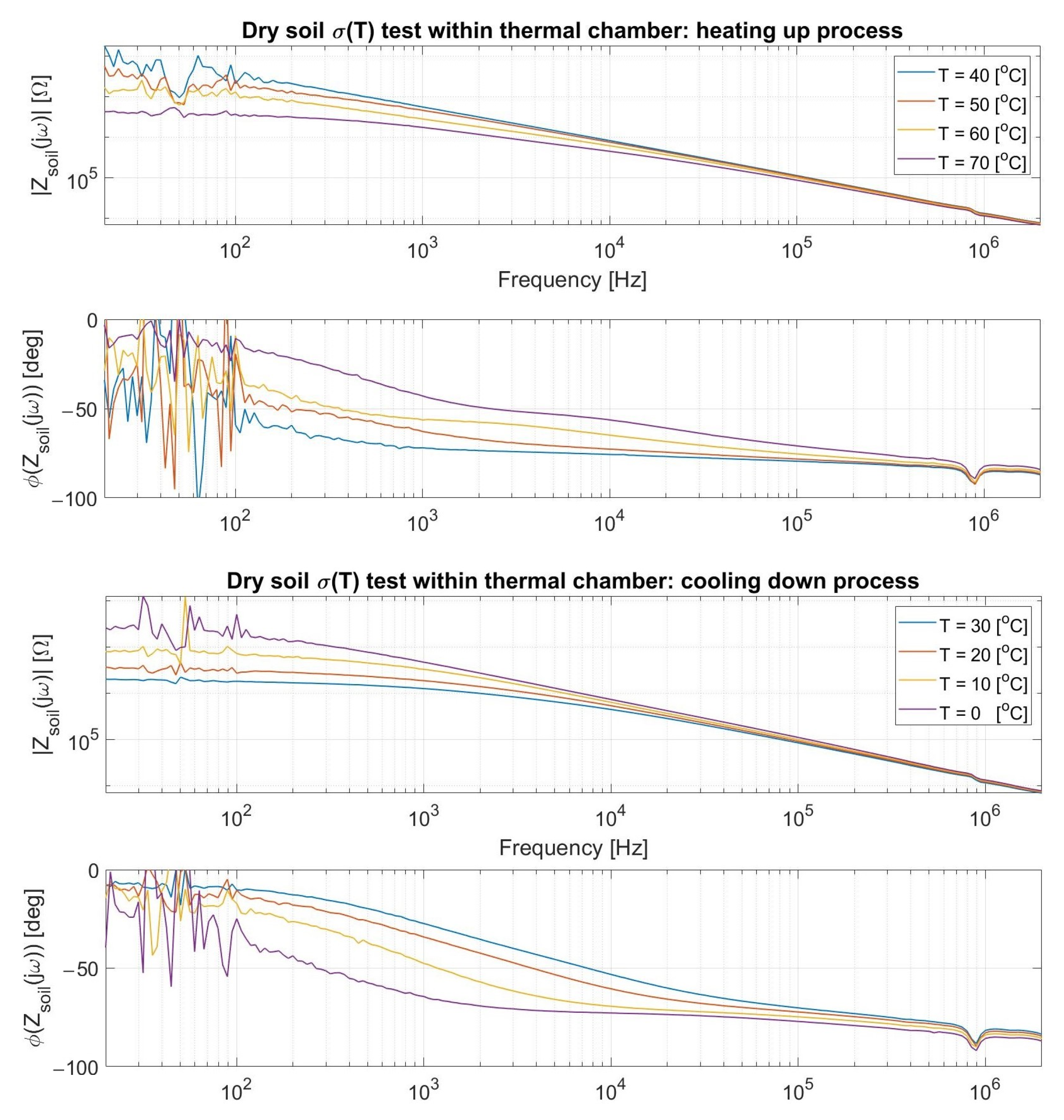
3.3.1. Temperature
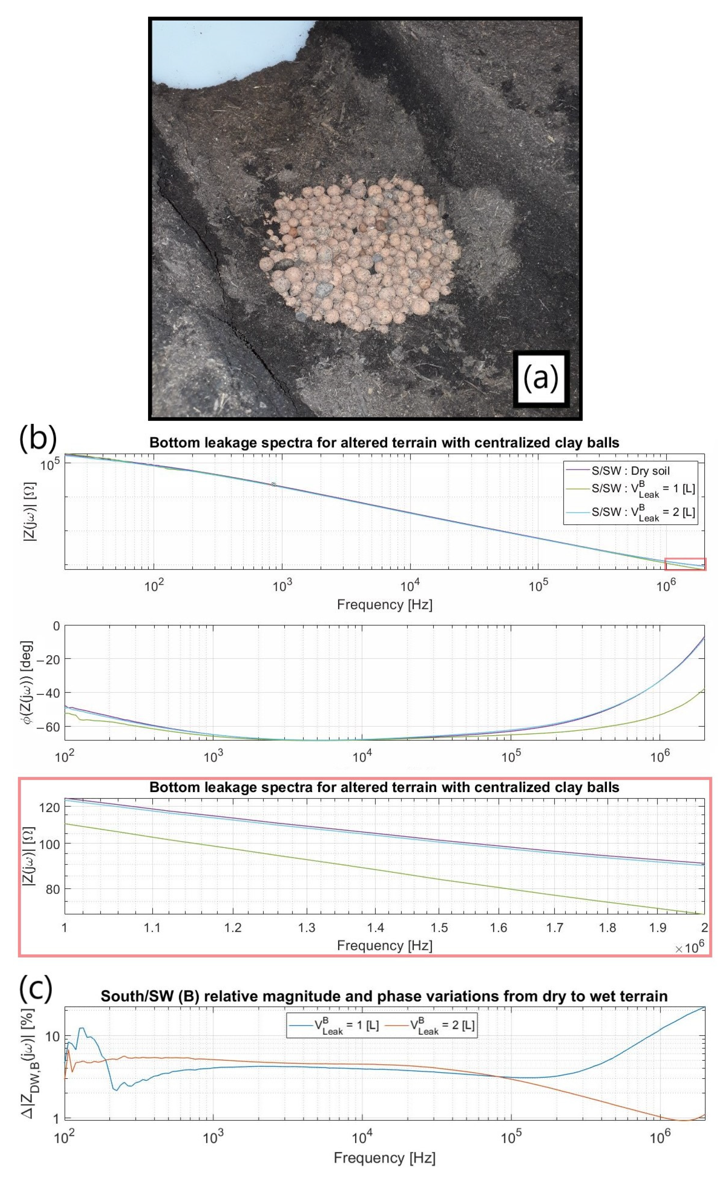
3.3.2. Soil Morphology
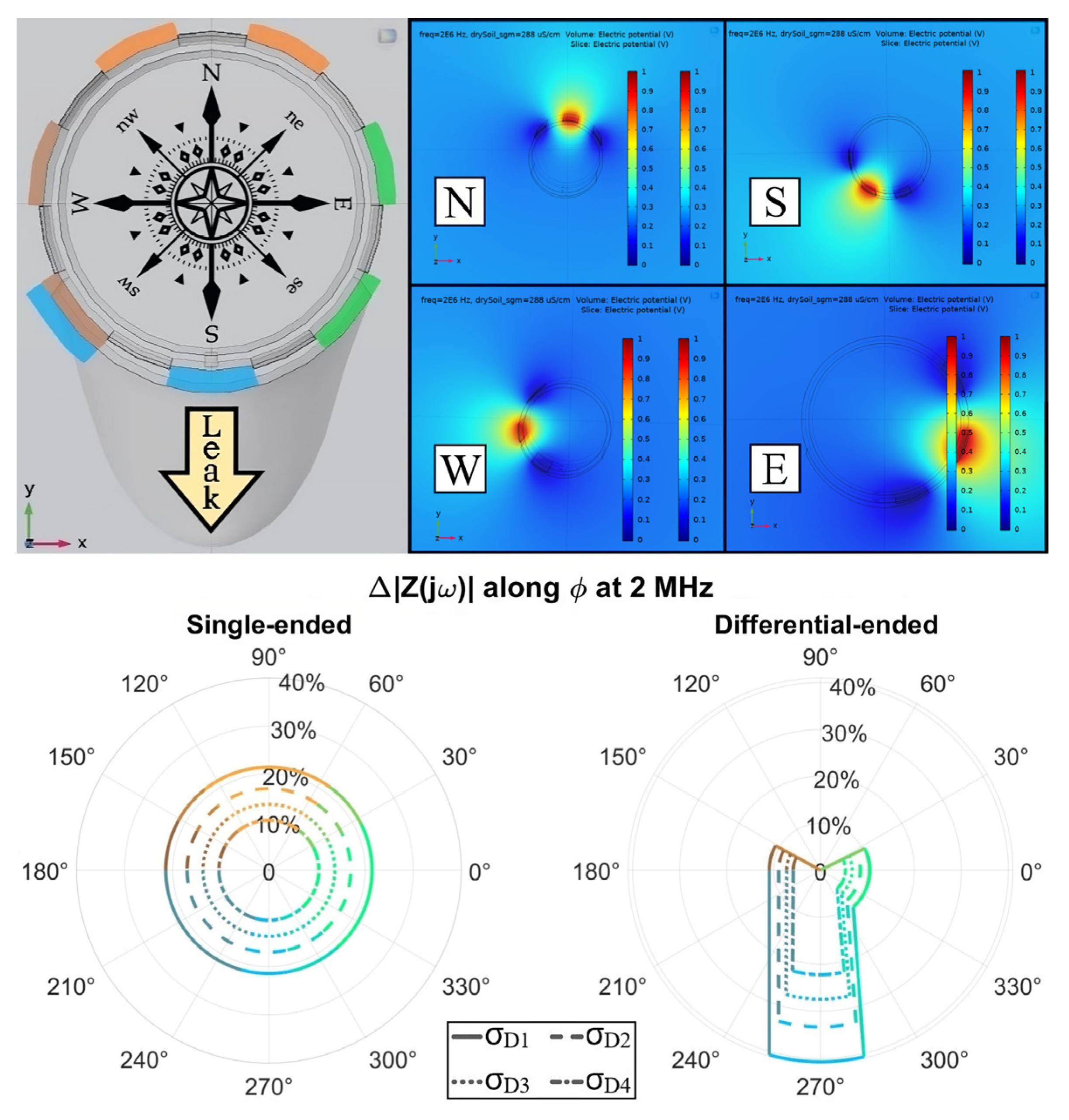
3.4. Differential Measurements
4. Discussion
5. Conclusions
Author Contributions
Funding
Institutional Review Board Statement
Informed Consent Statement
Data Availability Statement
Acknowledgments
Conflicts of Interest
References
- Hoekstra, A.Y.; Mekonnen, M.M. The Water Footprint of Humanity. Proc. Natl. Acad. Sci. USA 2012, 109, 3232–3237. [Google Scholar] [CrossRef] [PubMed] [Green Version]
- El-Zahab, S.; Zayed, T. Leak Detection in Water Distribution Networks: An Introductory Overview. Smart Water 2019, 4, 5. [Google Scholar] [CrossRef] [Green Version]
- Islam, M.R.; Azam, S.; Shanmugam, B.; Mathur, D. A Review on Current Technologies and Future Direction of Water Leakage Detection in Water Distribution Network. IEEE Access 2022, 10, 107177–107201. [Google Scholar] [CrossRef]
- Pudar, R.S.; Liggett, J.A. Leaks in Pipe Networks. J. Hydraul. Eng. 1992, 118, 1031–1046. [Google Scholar] [CrossRef]
- Levinas, D.; Perelman, G.; Ostfeld, A. Water Leak Localization Using High-Resolution Pressure Sensors. Water 2021, 13, 591. [Google Scholar] [CrossRef]
- Bach, P.M.; Kodikara, J.K. Reliability of Infrared Thermography in Detecting Leaks in Buried Water Reticulation Pipes. IEEE J. Sel. Top. Appl. Earth Obs. Remote Sens. 2017, 10, 4210–4224. [Google Scholar] [CrossRef]
- Sneddon, K.W.; Olhoeft, G.R.; Powers, M.H. Determlning And Mapplng Dnapl Saturation Values From Nonlnvasive Gpr Measurements. In Proceedings of the 13th EEGS Symposium on the Application of Geophysics to Engineering and Environmental Problems; European Association of Geoscientists & Engineers, Arlington, VA, USA, 20–24 February 2000. [Google Scholar]
- Okosun, F.; Cahill, P.; Hazra, B.; Pakrashi, V. Vibration-Based Leak Detection and Monitoring of Water Pipes Using Output-Only Piezoelectric Sensors. Eur. Phys. J. Spec. Top. 2019, 228, 1659–1675. [Google Scholar] [CrossRef]
- Gao, Y.; Brennan, M.J.; Joseph, P.F.; Muggleton, J.M.; Hunaidi, O. A Model of the Correlation Function of Leak Noise in Buried Plastic Pipes. J. Sound Vib. 2004, 277, 133–148. [Google Scholar] [CrossRef]
- Xu, J.; Chai, K.T.-C.; Wu, G.; Han, B.; Wai, E.L.-C.; Li, W.; Yeo, J.; Nijhof, E.; Gu, Y. Low-Cost, Tiny-Sized MEMS Hydrophone Sensor for Water Pipeline Leak Detection. IEEE Trans. Ind. Electron. 2019, 66, 6374–6382. [Google Scholar] [CrossRef]
- Mohd Ismail, M.I.; Dziyauddin, R.A.; Ahmad Salleh, N.A.; Muhammad-Sukki, F.; Aini Bani, N.; Mohd Izhar, M.A.; Latiff, L.A. A Review of Vibration Detection Methods Using Accelerometer Sensors for Water Pipeline Leakage. IEEE Access 2019, 7, 51965–51981. [Google Scholar] [CrossRef]
- Ren, L.; Jiang, T.; Jia, Z.; Li, D.; Yuan, C.; Li, H. Pipeline Corrosion and Leakage Monitoring Based on the Distributed Optical Fiber Sensing Technology. Measurement 2018, 122, 57–65. [Google Scholar] [CrossRef]
- Ibrahim, K.; Tariq, S.; Bakhtawar, B.; Zayed, T. Application of Fiber Optics in Water Distribution Networks for Leak Detection and Localization: A Mixed Methodology-Based Review. H2Open J. 2021, 4, 244–261. [Google Scholar] [CrossRef]
- Cataldo, A.; Persico, R.; Leucci, G.; De Benedetto, E.; Cannazza, G.; Matera, L.; De Giorgi, L. Time Domain Reflectometry, Ground Penetrating Radar and Electrical Resistivity Tomography: A Comparative Analysis of Alternative Approaches for Leak Detection in Underground Pipes. NDT E Int. 2014, 62, 14–28. [Google Scholar] [CrossRef]
- Jordana, J.; Gasulla, M.; Pallàs-Areny, R. Electrical Resistance Tomography to Detect Leaks from Buried Pipes. Meas. Sci. Technol. 2001, 12, 1061–1068. [Google Scholar] [CrossRef]
- D’Adda, I.; Battaglin, G.; Carminati, M. A Low-Cost Flexible Pipe Sheath for Multi-Parameter Monitoring of Water Distribution. In Proceedings of the 2021 IEEE International Symposium on Circuits and Systems (ISCAS), Daegu, Republic of Korea, 22–28 May 2021; IEEE: Daegu, Republic of Korea, 2021; pp. 1–5. [Google Scholar]
- Luo, B.; Wang, T.; Zhang, F.; Lin, Y.; Zheng, C.; Chen, S. Interdigital Capacitive Sensor for Cable Insulation Defect Detection: Three-Dimensional Modeling, Design, and Experimental Test. J. Sens. 2021, 2021, 8859742. [Google Scholar] [CrossRef]
- Quan, J.; Shi, X.; Kim, K.N.; Oh, D.S.; Chua, B. Electrically Functional Water Sensing Duct Tape Suitable for Detection of Indoor Pinhole Leakages with High Spatial and Temporal Resolution. Sens. Actuators A Phys. 2023, 351, 114145. [Google Scholar] [CrossRef]
- Carminati, M.; Ferrari, G.; Vahey, M.D.; Voldman, J.; Sampietro, M. Miniaturized Impedance Flow Cytometer: Design Rules and Integrated Readout. IEEE Trans. Biomed. Circuits Syst. 2017, 11, 1438–1449. [Google Scholar] [CrossRef]
- Carminati, M.; Mezzera, L.; Turolla, A.; Pani, G.; Tizzoni, M.; Di Mauro, M.; Antonelli, M. Flexible Impedance Sensor for In-Line Monitoring of Water and Beverages. In Proceedings of the 2019 IEEE International Symposium on Circuits and Systems (ISCAS), Sapporo, Japan, 26–29 May 2019; IEEE: Sapporo, Japan, 2019; pp. 1–4. [Google Scholar]
- Riboldi, C.; Castillo, D.A.C.; Crafa, D.M.; Carminati, M. Contactless Sensing of Water Properties for Smart Monitoring of Pipelines. Sensors 2023, 23, 2075. [Google Scholar] [CrossRef]
- Demierre, N.; Braschler, T.; Linderholm, P.; Seger, U.; van Lintel, H.; Renaud, P. Characterization and Optimization of Liquid Electrodes for Lateral Dielectrophoresis. Lab Chip 2007, 7, 355–365. [Google Scholar] [CrossRef]
- Cho, T.-S.; Choi, K.-S.; Seo, D.-C.; Kwon, I.-B.; Lee, J.-R. Novel Fiber Optic Sensor Probe with a Pair of Highly Reflected Connectors and a Vessel of Water Absorption Material for Water Leak Detection. Sensors 2012, 12, 10906–10919. [Google Scholar] [CrossRef] [Green Version]
- Pietrosanto, A.; Carratù, M.; Liguori, C. Sensitivity of Water Meters to Small Leakage. Measurement 2021, 168, 108479. [Google Scholar] [CrossRef]
- Casillas Ponce, M.V.; Garza Castañón, L.E.; Cayuela, V.P. Model-Based Leak Detection and Location in Water Distribution Networks Considering an Extended-Horizon Analysis of Pressure Sensitivities. J. Hydroinform. 2014, 16, 649–670. [Google Scholar] [CrossRef] [Green Version]
- Fan, X.; Zhang, X.; Yu, X. Machine Learning Model and Strategy for Fast and Accurate Detection of Leaks in Water Supply Network. J. Infrastruct. Preserv. Resil. 2021, 2, 10. [Google Scholar] [CrossRef]


| Z () = zG |
| ZSoil @1kHz (σL, hL) | VLeak = 0.25 [L] (hL~7.3 [cm]) | VLeak = 0.5 [L] (hL~12.4 [cm]) | VLeak = 0.75 [L] (hL~16.5 [cm]) | VLeak = 1.0 [L] (hL~20 [cm]) |
|---|---|---|---|---|
| 1.0 (BL) | 20,426 ∠ −0.82° | 20,426 ∠ −0.82° | 20,426 ∠ −0.82° | 20,426 ∠ −0.82° |
| 25.0 | 12,755 ∠ −0.50° | 12,715 ∠ −0.50° | 12,706 ∠ −0.50° | 12,701 ∠ −0.50° |
| 50.0 | 9293 ∠ −0.37° | 9268 ∠ −0.36° | 9264 ∠ −0.36° | 9260 ∠ −0.36° |
| 100.0 | 6030 ∠ −0.24° | 6016 ∠ −0.24° | 6015 ∠ −0.24° | 6013 ∠ −0.24° |
| 150.0 | 4463 ∠ −0.18° | 4455 ∠ −0.18° | 4454 ∠ −0.18° | 4453 ∠ −0.18° |
| 200.0 | 3544 ∠ −0.14° | 3537 ∠ −0.14° | 3537 ∠ −0.14° | 3536 ∠ −0.14° |
| 300.0 | 2509 ∠ −0.10° | 2505 ∠ −0.10° | 2505 ∠ −0.10° | 2504 ∠ −0.10° |
| 400.0 | 1942 ∠ −0.08° | 1939 ∠ −0.08° | 1939 ∠ −0.08° | 1938 ∠ −0.08° |
| 500.0 | 1584 ∠ −0.06° | 1582 ∠ −0.06° | 1582 ∠ −0.06° | 1581 ∠ −0.06° |
| ZSoil(jω) | Dry (BL) | 0.5 [L] | 1.0 [L] | 1.5 [L] | 2.0 [L] | 3.0 [L] | 4.0 [L] |
|---|---|---|---|---|---|---|---|
| Δ|ZDW(jω)| | |||||||
| 5 [cm] | 129.6 ∠−24.4° | 117.9 ∠−24.5° | 108.8 ∠−25.9° | 99.9 ∠−27.0° | 88.3 ∠−29.0° | -- | -- |
| 0% | 9.0% | 16.1% | 22.9% | 31.9% | |||
| 17 [cm] | 55.8 ∠−13.6° | -- | 50.5 ∠−12.5° | -- | 48.5 ∠−11.8° | 47.5 ∠−11.1° | 47.0 ∠−10.7° |
| 0% | 9.5% | 13.1% | 14.9% | 15.8% |
| Materials | ρSoil = 5 [cm] | ρSoil =17 [cm] | ||
|---|---|---|---|---|
| Dry | Wet | Dry | Wet | |
| Ground (1) | σ = 45 εr = 7.5 | σ = 400 εr = 60 | σ = 180 εr = 2.5 | σ ∊ [300, 400] εr = 60 |
| Ionic double Layer (2) | σ = 115 ε = 0.35 | σ = 400 ε = 0.5 | σ = 20 εr = α εKp(jω)−0.17, α = 2, εKp = 3 | σ = 50 εr = α εKp(jω)−0.17 α > 2 (α ∊ ℝ), εKp = 3 |
| Kapton® (2) | σ = 115 εr = 3 (3) | σ = 115 εr = 3 | ||
| |Z(jω)|[Ω] | σD1 (180 [μS/cm]) | σD2 (216 [μS/cm]) | σD3 (252 [μS/cm]) | σD4 (288 [μS/cm]) |
|---|---|---|---|---|
| S.E. Dry BL | 38.68 | 32.51 | 28.11 | 24.81 |
| S.E. Wet | 30.38 | 26.98 | 24.33 | 22.22 |
| D.E. Dry BL | 104.50 | 87.80 | 75.88 | 66.95 |
| D.E. (N) Wet | 104.49 | 87.79 | 75.88 | 66.95 |
| D.E. (W) Wet | 93.07 | 79.99 | 70.41 | 63.08 |
| D.E. (S) Wet | 62.77 | 58.55 | 55.06 | 52.10 |
| D.E. (E) Wet | 93.50 | 80.37 | 70.76 | 63.40 |
| Technology | L [m] | V [L] | t [s] | FoM * | Ref. |
|---|---|---|---|---|---|
| Impedance | 6 | 0.5 | 1 | 12 | This work |
| Optical Fiber | 0.02 | 0.005 | 600 | 0.007 | [23] |
| Smart Meter | 1 | 0.008 | 10 | 12.8 | [24] |
| Pressure | 100 | 7 | 10 | 1.4 | [25] |
Disclaimer/Publisher’s Note: The statements, opinions and data contained in all publications are solely those of the individual author(s) and contributor(s) and not of MDPI and/or the editor(s). MDPI and/or the editor(s) disclaim responsibility for any injury to people or property resulting from any ideas, methods, instructions or products referred to in the content. |
© 2023 by the authors. Licensee MDPI, Basel, Switzerland. This article is an open access article distributed under the terms and conditions of the Creative Commons Attribution (CC BY) license (https://creativecommons.org/licenses/by/4.0/).
Share and Cite
Carnevale Castillo, D.A.; Carminati, M. A Pipe-Embeddable Impedance Sensor for Monitoring Water Leaks in Distribution Networks: Design and Validation. Sensors 2023, 23, 3117. https://doi.org/10.3390/s23063117
Carnevale Castillo DA, Carminati M. A Pipe-Embeddable Impedance Sensor for Monitoring Water Leaks in Distribution Networks: Design and Validation. Sensors. 2023; 23(6):3117. https://doi.org/10.3390/s23063117
Chicago/Turabian StyleCarnevale Castillo, Danilo Aparecido, and Marco Carminati. 2023. "A Pipe-Embeddable Impedance Sensor for Monitoring Water Leaks in Distribution Networks: Design and Validation" Sensors 23, no. 6: 3117. https://doi.org/10.3390/s23063117