


Performance of Different Crop Models in Simulating Soil Temperature


Abstract
:1. Introduction
2. Methodology
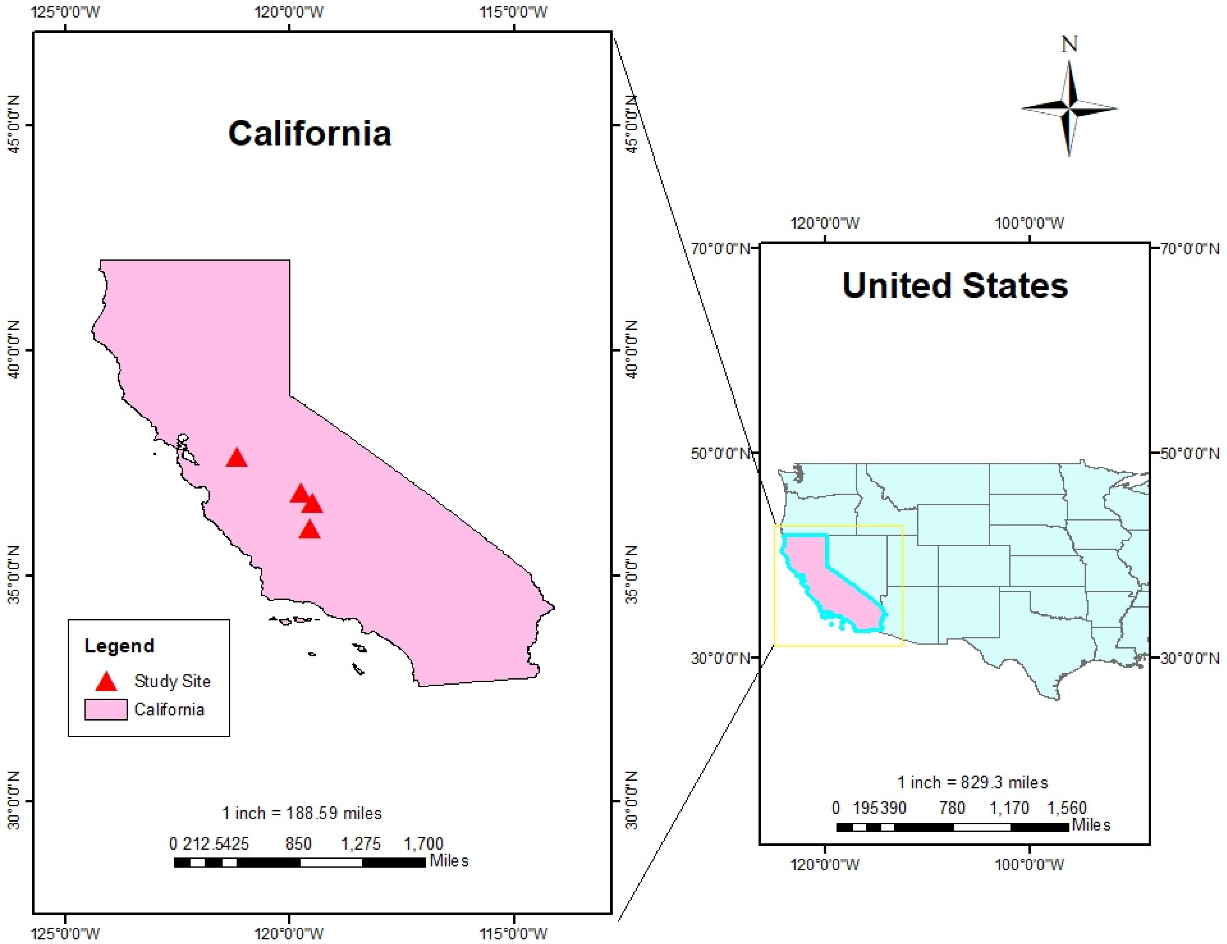
2.1. Study Sites
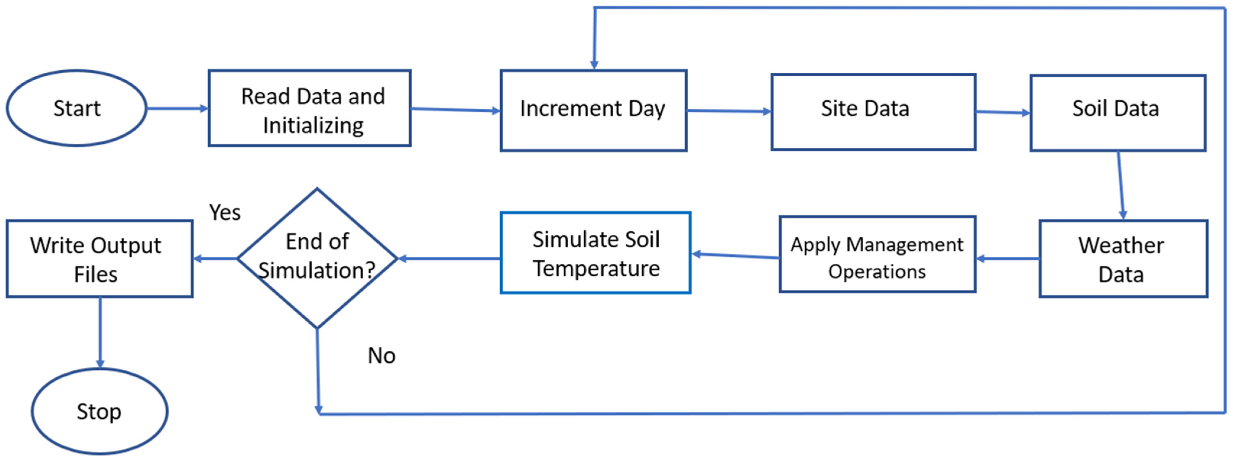
2.2. Experimental Set-Up
2.2.1. Noah-MP
2.2.2. EPIC
2.3. Model Evaluation
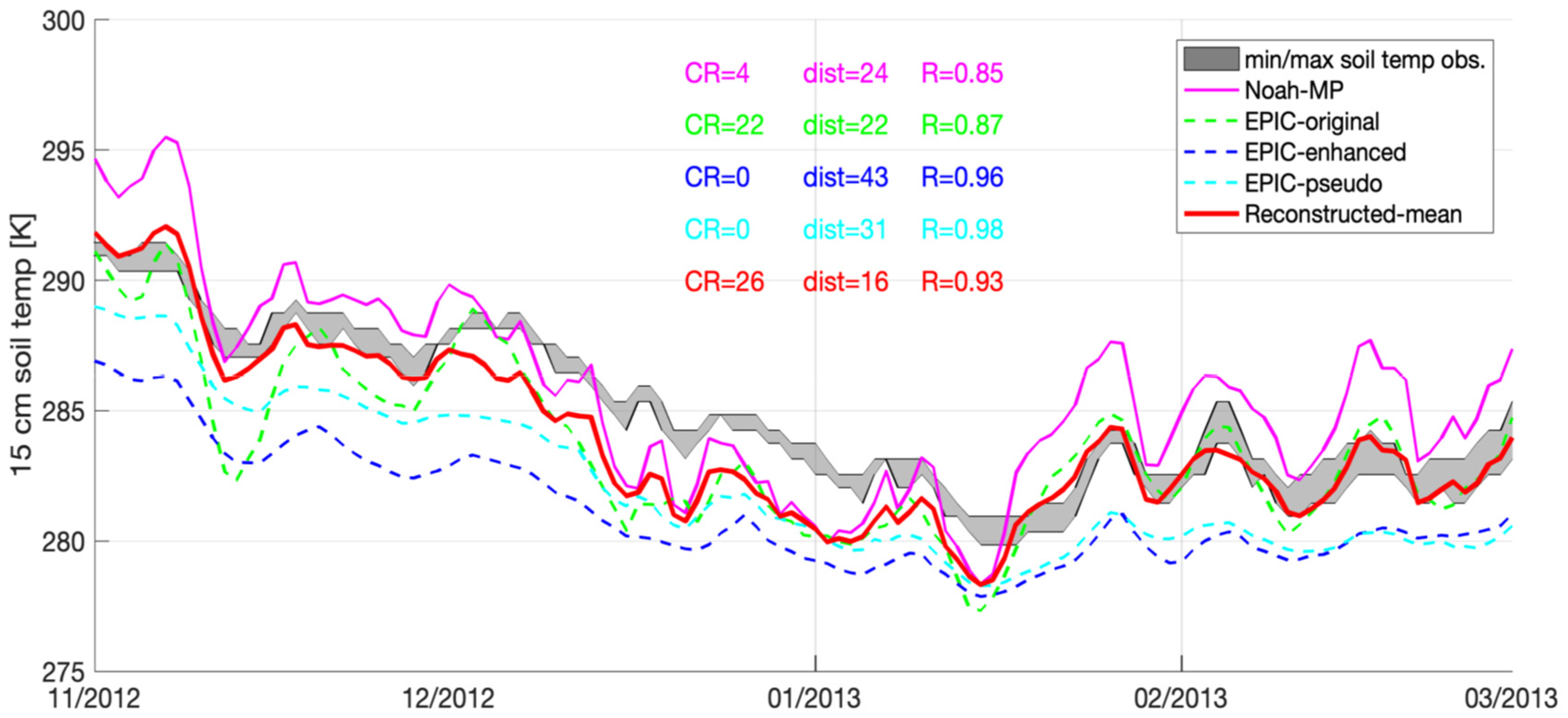
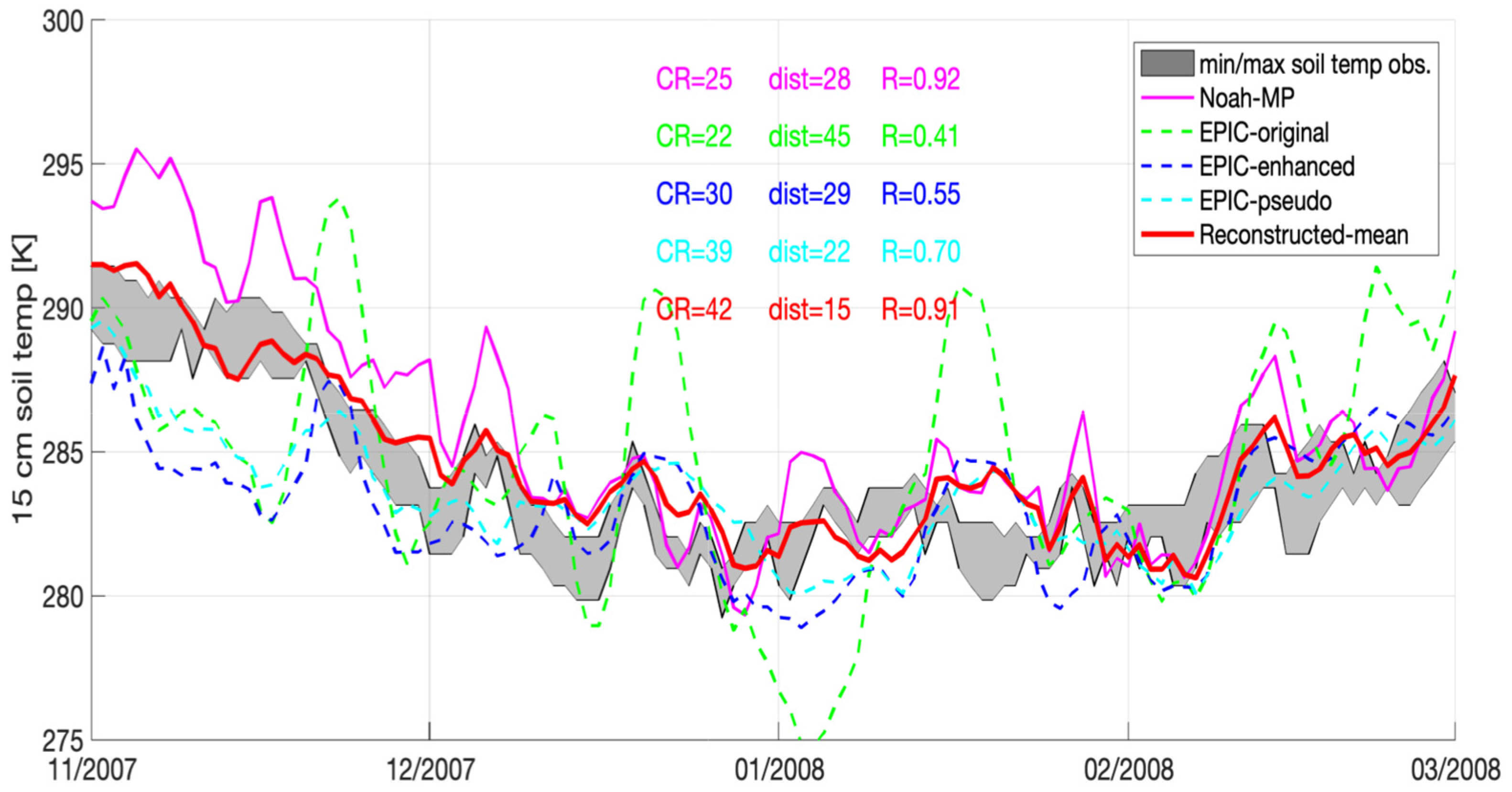
3. Results
4. Discussion
5. Conclusions
Author Contributions
Funding
Institutional Review Board Statement
Informed Consent Statement
Data Availability Statement
Conflicts of Interest
References
- Fereres, E.; Orgaz, F.; Gonzalez-Dugo, V. Reflections on food security under water scarcity. J. Exp. Bot. 2011, 62, 4079–4086. [Google Scholar] [CrossRef] [PubMed] [Green Version]
- Bell, J.E.; Autry, C.W.; Mollenkopf, D.A.; Thornton, L.M. A Natural Resource Scarcity Typology: Theoretical Foundations and Stra-tegic Implications for Supply Chain Management: A Natural Resource Scarcity Typology. J. Bus. Logist. 2012, 33, 158–166. [Google Scholar] [CrossRef]
- Jones, B.T.; Mattiacci, E.; Braumoeller, B.F. Food scarcity and state vulnerability: Unpacking the link between climate variability and violent unrest. J. Peace Res. 2017, 54, 335–350. [Google Scholar] [CrossRef]
- Kummu, M.; Guillaume, J.H.A.; de Moel, H.; Eisner, S.; Flörke, M.; Porkka, M.; Siebert, S.; Veldkamp, T.I.E.; Ward, P.J. The world’s road to water scarcity: Shortage and stress in the 20th century and pathways towards sustainability. Sci. Rep. 2016, 6, 38495. [Google Scholar] [CrossRef] [Green Version]
- Marston, L.T.; Read, Q.D.; Brown, S.P.; Muth, M.K. Reducing Water Scarcity by Reducing Food Loss and Waste. Front. Sustain. Food Syst. 2021, 5, 1476. [Google Scholar] [CrossRef]
- Amusan, L.; Oyewole, S. Precision agriculture and the prospects of space strategy for food security in Africa. Afr. J. Sci. Technol. Innov. Dev. 2022, 1–12. [Google Scholar] [CrossRef]
- Kirkaya, A. Smart farming- precision agriculture technologies and practices. JSP 2020, 4, 123–136. [Google Scholar] [CrossRef]
- Trivelli, L.; Apicella, A.; Chiarello, F.; Rana, R.; Fantoni, G.; Tarabella, A. From precision agriculture to Industry 4.0: Unveiling technological connections in the agrifood sector. BFJ 2019, 121, 1730–1743. [Google Scholar] [CrossRef]
- Kehl, J. Moving beyond the Mirage: Water Scarcity and Agricultural Use Inefficiency in USA. Water 2020, 12, 2290. [Google Scholar] [CrossRef]
- Thenkabail, P.S. Global Croplands and their Importance for Water and Food Security in the Twenty-first Century: Towards an Ever Green Revolution that Combines a Second Green Revolution with a Blue Revolution. Remote Sens. 2010, 2, 2305–2312. [Google Scholar] [CrossRef] [Green Version]
- Shu, L.; Hancke, G.P.; Abu-Mahfouz, A.M. Guest Editorial: Sustainable and Intelligent Precision Agriculture. IEEE Trans. Ind. Inform. 2021, 17, 4318–4321. [Google Scholar] [CrossRef]
- Lee, C.L.; Strong, R.; Dooley, K.E. Analyzing Precision Agriculture Adoption across the Globe: A Systematic Review of Scholar-ship from 1999–2020. Sustainability 2021, 13, 10295. [Google Scholar] [CrossRef]
- Linaza, M.T.; Posada, J.; Bund, J.; Eisert, P.; Quartulli, M.; Döllner, J.; Pagani, A.; Olaizola, I.G.; Barriguinha, A.; Moysiadis, T.; et al. Data-Driven Artificial Intelligence Applications for Sus-tainable Precision Agriculture. Agronomy 2021, 11, 1227. [Google Scholar] [CrossRef]
- Mafuta, M.; Zennaro, M.; Bagula, A.; Ault, G.; Gombachika, H.; Chadza, T. Successful deployment of a Wireless Sensor Network for precision agriculture in Malawi. In Proceedings of the IEEE 3rd International Conference on Networked Embedded Systems for Every Application (NESEA), Liverpool, UK, 13–14 December 2012; pp. 1–7. [Google Scholar] [CrossRef] [Green Version]
- Miles, C. The combine will tell the truth: On precision agriculture and algorithmic rationality. Big Data Soc. 2019, 1–12. [Google Scholar] [CrossRef] [Green Version]
- Awasthi, A.; Reddy, S.R.N. Monitoring for Precision Agriculture using Wireless Sensor Network—A Review. Glob. J. Comput. Sci. Technol. 2013, 23–28. [Google Scholar]
- Precision Agriculture: Tomorrow’s Technology for Today’s Farmer. J. Food Process. Technol. 2015, 6, 1000648. Available online: https://www.omicsonline.org/open-access/precision-agriculture-tomorrows-technology-for-todays-farmer-2157-7110-1000468.php?aid=58751 (accessed on 6 April 2022).
- Shafi, U.; Mumtaz, R.; García-Nieto, J.; Hassan, S.A.; Zaidi, S.A.R.; Iqbal, N. Precision Agriculture Techniques and Practices: From Considerations to Applications. Sensors 2019, 19, 3796. [Google Scholar] [CrossRef] [PubMed] [Green Version]
- Onwuka, B. Effects of Soil Temperature on Some Soil Properties and Plant Growth. APAR 2018, 8, 34–37. Available online: https://medcraveonline.com/APAR/effects-of-soil-temperature-on-some-soil-properties-and-plant-growth.html (accessed on 6 April 2022). [CrossRef]
- Schoonover, J.E.; Crim, J.F. An Introduction to Soil Concepts and the Role of Soils in Watershed Management. J. Contemp. Water Res. Educ. 2015, 154, 21–47. [Google Scholar] [CrossRef] [Green Version]
- Dong, X.; Xu, W.; Zhang, Y.; Leskovar, D.I. Effect of Irrigation Timing on Root Zone Soil Temperature, Root Growth and Grain Yield and Chemical Composition in Corn. Agronomy 2016, 6, 34. [Google Scholar] [CrossRef] [Green Version]
- Adak, T.; Kumar, G.; Sharma, P.K.; Srivastava, A.K.; Chakravarty, N. Seasonal changes in soil temperature within mustard crop stand. J. Agrometeorol. 2011, 13, 72–74. [Google Scholar] [CrossRef]
- Oliveira, J.; Timm, L.; Tominaga, T.; Cássaro, F.; Reichardt, K.; Bacchi, O.; Neto, D.D.; Câmara, G.D.S. Soil temperature in a sugar-cane crop as a function of the management system. Plant Soil 2001, 230, 61–66. [Google Scholar] [CrossRef]
- Alvarado, V.; Bradford, K.J. A hydrothermal time model explains the cardinal temperatures for seed germination: Hydrother-mal time model of seed germination. Plant Cell Environ. 2002, 25, 1061–1069. [Google Scholar] [CrossRef]
- Doro, L.; Wang, X.; Ammann, C.; De Antoni Migliorati, M.; Grünwald, T.; Klumpp, K.; Loubet, B.; Pattey, E.; Wohlfahrt, G.; Williams, J.R.; et al. Improving the simulation of soil temperature within the EPIC model. Environ. Model. Softw. 2021, 144, 105140. [Google Scholar] [CrossRef]
- Smith, W.N.; Grant, B.B.; Desjardins, R.L.; Rochette, P.; Drury, C.F.; Li, C. Evaluation of two process-based models to estimate soil N2O emissions in Eastern Canada. Can. J. Soil Sci. 2008, 88, 251–260. [Google Scholar] [CrossRef]
- Archontoulis, S.V.; Miguez, F.E.; Moore, K.J. Evaluating APSIM Maize, Soil Water, Soil Nitrogen, Manure, and Soil Temperature Modules in the Midwestern United States. Agron. J. 2014, 106, 1025–1040. [Google Scholar] [CrossRef]
- Xia, Y.; Ek, M.; Sheffield, J.; Livneh, B.; Huang, M.; Wei, H.; Feng, S.; Luo, L.; Meng, J.; Wood, E. Validation of Noah-Simulated Soil Temperature in the North American Land Data Assimilation System Phase 2. J. Appl. Meteorol. Clim. 2013, 52, 455–471. [Google Scholar] [CrossRef] [Green Version]
- Stefan, V.; Merlin, O.; Er-Raki, S.; Escorihuela, M.J.; Khabba, S. Consistency between In Situ, Model-Derived and High-Resolution-Image-Based Soil Temperature Endmembers: Towards a Robust Data-Based Model for Multi-Resolution Monitoring of Crop Evap-otranspiration. Remote Sens. 2015, 7, 10444–10479. [Google Scholar] [CrossRef] [Green Version]
- Arsenault, R.; Essou, G.R.C.; Brissette, F.P. Improving Hydrological Model Simulations with Combined Multi-Input and Multimodel Averaging Frameworks. J. Hydrol. Eng. 2017, 04016066-1–04016066-11. [Google Scholar] [CrossRef]
- Arsenault, R.; Gatien, P.; Renaud, B.; Brissette, F.; Martel, J.-L. A comparative analysis of 9 multi-model averaging approaches in hydrological continuous streamflow simulation. J. Hydrol. 2015, 529, 754–767. [Google Scholar] [CrossRef]
- Lambert, S.J.; Boer, G.J. CMIP1 evaluation and intercomparison of coupled climate models. Clim. Dyn. 2001, 17, 83–106. [Google Scholar] [CrossRef]
- Nicolle, P.; Pushpalatha, R.; Perrin, C.; François, D.; Thiéry, D.; Mathevet, T.; Le Lay, M.; Besson, F.; Soubeyroux, J.-M.; Viel, C.; et al. Benchmarking hydrological models for low-flow simulation and forecasting on French catchments. Hydrol. Earth Syst. Sci. 2014, 18, 2829–2857. [Google Scholar] [CrossRef] [Green Version]
- Bandaru, V.; Yaramasu, R.; Jones, C.; César Izaurralde, R.; Reddy, A.; Sedano, F.; Daughtry, C.S.; Becker-Reshef, I.; Justice, C. Geo-CropSim: A Geo-spatial crop simula-tion modeling framework for regional scale crop yield and water use assessment. ISPRS J. Photogramm. Remote Sens. 2022, 183, 34–53. [Google Scholar] [CrossRef]
- Cabelguenne, M.; Jones, C.A.; Marty, J.R.; Dyke, P.T.; Williams, J.R. Calibration and validation of EPIC for crop rotations in southern France. Agric. Syst. 1990, 33, 153–171. [Google Scholar] [CrossRef]
- Kiniry, J.R.; Blanchet, R.; Williams, J.R.; Texier, V.; Jones, C.A.; Cabelguenne, M. Sunflower simulation using the EPIC and ALMA-NAC models. Field Crops Res. 1992, 30, 403–423. [Google Scholar] [CrossRef]
- Potter, K.N.; Williams, J.R.; Larney, F.J.; Bullock, M.S. Evaluation of EPIC’s wind erosion submodel using data from southern Al-berta. Can J Soil Sci. 1998, 78, 485–492. [Google Scholar] [CrossRef]
- Rasche, L.; Taylor, R.A.J. EPIC-GILSYM: Modelling crop-pest insect interactions and management with a novel coupled crop-insect model. J. Appl. Ecol. 2019, 13426, 1365–2664. [Google Scholar] [CrossRef]
- Rinaldi, M. Application of EPIC model for irrigation scheduling of sun¯ower in Southern Italy. Agric. Water Manag. 2001, 12, 185–196. [Google Scholar] [CrossRef]
- Roloff, G.; Dejong, R.; Nolin, M.C. Crop yield, soil temperature and sensitivity of EPIC under central-eastern Canadian condi-tions. Can. J. Soil Sci. 1998, 78, 431–439. [Google Scholar] [CrossRef]
- Izaurralde, R.C.; Williams, J.R.; McGill, W.B.; Rosenberg, N.J.; Jakas, M.C.Q. Simulating soil C dynamics with EPIC: Model descrip-tion and testing against long-term data. Ecol. Model. 2006, 192, 362–384. [Google Scholar] [CrossRef]
- Chen, L.; Li, Y.; Chen, F.; Barr, A.; Barlage, M.; Wan, B. The incorporation of an organic soil layer in the Noah-MP land surface modeland its evaluation over a boreal aspen forest. Atmos. Chem. Phys. 2016, 16, 8375–8387. [Google Scholar] [CrossRef] [Green Version]
- Liu, X.; Chen, F.; Barlage, M.; Zhou, G.; Niyogi, D. Noah-MP-Crop: Introducing dynamic crop growth in the Noah-MP land sur-face model: Noah-MP-Crop. J. Geophys. Res. Atmos. 2016, 121, 13953–13972. [Google Scholar] [CrossRef] [Green Version]
- Ahmed, M.; Stöckle, C.O.; Nelson, R.; Higgins, S. Assessment of Climate Change and Atmospheric CO2 Impact on Winter Wheat in the Pacific Northwest Using a Multimodel Ensemble. Front. Ecol. Evol. 2017, 5, 51. [Google Scholar] [CrossRef] [Green Version]
- Xue, Y.; Houser, P.R.; Maggioni, V.; Mei, Y.; Kumar, S.V.; Yoon, Y. Assimilation of Satellite-Based Snow Cover and Freeze/Thaw Observations Over High Mountain Asia. Front. Earth Sci. 2019, 7, 115. [Google Scholar] [CrossRef] [PubMed] [Green Version]
- Li, X.; Wu, T.; Zhu, X.; Jiang, Y.; Hu, G.; Hao, J.; Ni, J.; Li, R.; Qiao, Y.; Yang, C.; et al. Improving the Noah-MP Model for Simulating Hydrothermal Regime of the Active Layer in the Permafrost Regions of the Qinghai-Tibet Plateau. J. Geophys. Res. Atmos. 2020, 125, e2020JD032588. [Google Scholar] [CrossRef]
- Guan, Y.; Shen, Y.; Mohammadi, B.; Sadat, M.A. Estimation of Soil Temperature Based on Meteorological Parameters by the HY-BRID INVASIVE Weed Optimization Algorithm Model. IOP Conf. Ser. Earth Environ. Sci. 2020, 428, 012059. [Google Scholar] [CrossRef]
- Jimeno-Sáez, P.; Senent-Aparicio, J.; Pérez-Sánchez, J.; Pulido-Velazquez, D. A Comparison of SWAT and ANN Models for Dai-ly Runoff Simulation in Different Climatic Zones of Peninsular Spain. Water 2018, 10, 192. [Google Scholar] [CrossRef] [Green Version]
- Shortridge, J.E.; Guikema, S.D.; Zaitchik, B.F. Machine learning methods for empirical streamflow simulation: A comparison of model accuracy, interpretability, and uncertainty in seasonal watersheds. Hydrol. Earth Syst. Sci. 2016, 20, 2611–2628. [Google Scholar] [CrossRef] [Green Version]
- Tabari, H.; Marofi, S.; Ahmadi, M. Long-term variations of water quality parameters in the Maroon River, Iran. Environ. Monit. Assess. 2010, 177, 273–287. [Google Scholar] [CrossRef]
- Diffenbaugh, N.S.; Swain, D.L.; Touma, D. Anthropogenic warming has increased drought risk in California. Proc. Natl. Acad. Sci. USA 2015, 112, 3931–3936. [Google Scholar] [CrossRef] [PubMed] [Green Version]
- Luo, L.; Apps, D.; Arcand, S.; Xu, H.; Pan, M.; Hoerling, M. Contribution of temperature and precipitation anomalies to the Cali-fornia drought during 2012-2015: Contribution of T and P to CA drought. Geophys. Res. Lett. 2017, 44, 3184–3192. [Google Scholar] [CrossRef]
- Mann, M.E.; Gleick, P.H. Climate change and California drought in the 21st century. Proc. Natl. Acad. Sci. USA 2015, 112, 3858–3859. [Google Scholar] [CrossRef] [PubMed] [Green Version]
- Reiter, M.E.; Elliott, N.K.; Jongsomjit, D.; Golet, G.H.; Reynolds, M.D. Impact of extreme drought and incentive programs on flood-ed agriculture and wetlands in California’s Central Valley. PeerJ 2018, 6, e5147. [Google Scholar] [CrossRef] [PubMed]
- Robeson, S.M. Revisiting the recent California drought as an extreme value. Geophys. Res. Lett. 2015, 42, 6771–6779. [Google Scholar] [CrossRef]
- Williams, A.P.; Seager, R.; Abatzoglou, J.T.; Cook, B.I.; Smerdon, J.E.; Cook, E.R. Contribution of anthropogenic warming to Califor-nia drought during 2012–2014. Geophys. Res. Lett. 2015, 42, 6819–6828. [Google Scholar] [CrossRef] [Green Version]
- Kumar, S.; Peters-Lidard, C.; Tian, Y.; Houser, P.; Geiger, J.; Olden, S.; Lighty, L.; Eastman, J.; Doty, B.; Dirmeyer, P. Land information system: An interoperable framework for high resolution land surface modeling. Environ. Model. Softw. 2006, 21, 1402–1415. [Google Scholar] [CrossRef]
- Reichle, R.H.; Liu, Q.; Koster, R.D.; Draper, C.S.; Mahanama, S.P.P.; Partyka, G.S. Land Surface Precipitation in MERRA-2. J. Clim. 2017, 30, 1643–1664. [Google Scholar] [CrossRef]
- Cosgrove, B.A.; Lohmann, D.; Mitchell, K.E.; Houser, P.R.; Wood, E.F.; Schaake, J.C.; Robock, A.; Marshall, C.; Sheffield, J.; Duan, Q.Y.; et al. Real-time and retrospective forcing in the North American Land Data Assimilation System (NLDAS) project. J. Geophys. Res. Atmos. 2003, 108, 8842. [Google Scholar] [CrossRef] [Green Version]
- Case, J.L.; Crosson, W.L.; Kumar, S.V.; Lapenta, W.M.; Peters-Lidard, C.D. Impacts of High-Resolution Land Surface Initialization on Regional Sensible Weather Forecasts from the WRF Model. J. Hydrometeorol. 2008, 9, 1249–1266. [Google Scholar] [CrossRef]
- Niu, G.Y.; Yang, Z.L.; Mitchell, K.E.; Chen, F.; Ek, M.B.; Barlage, M.; Kumar, A.; Manning, K.; Niyogi, D.; Rosero, E.; et al. The community Noah land surface model with multipa-rameterization options (Noah-MP): 1. Model description and evaluation with local-scale measurements. J. Geophys. Res. 2011, 116, D12109. [Google Scholar] [CrossRef] [Green Version]
- Putman, J.; Williams, J.; Sawyer, D. Using the erosion-productivity impact calculator (EPIC) model to estimate the impact of soil erosion for the 1985 RCA appraisal. J. Soil Water Conserv. 1988, 6, 321–326. [Google Scholar]
- Brown, R.A.; Rosenberg, N.J. Climate Change Impacts on the Potential Productivity of Corn and Winter Wheat in Their Primary United States Growing Regions. Clim. Chang. 1999, 41, 73–107. [Google Scholar] [CrossRef]
- Taylor, J.R. An Introduction to Error Analysis: The Study of Uncertainties in Physical Measurements, 2nd ed.; University Science Books: Sausalito, CA, USA, 1997; 327p. [Google Scholar]


| References | Model | Study Area | Year | Coupled Model | Simulated Parameter | Conclusion |
|---|---|---|---|---|---|---|
| [40] | EPIC | Two sites in Ontario and Quebec, Canada | 1987–1995 | No | Crop Yield (using different Potential Evapotranspiration estimation) and Soil Temperature | Adequate estimation of yield (soybean and corn), Under-prediction of soil temperature |
| [37] | EPIC | Alberta, Canada | 1992 | No | Wind Erosion | Not accurately simulated |
| [39] | EPIC | Experimental Farm in Foggia at Italy | 1953 to 1997 | No | Yield, Water use efficiency and economic analysis (from the yield) | Reliable estimates, Good Basis for Decision Support at farm level |
| [41] | EPIC | Five sites in the USA and one site in Breton, Canada | 1938–1998 | No | Soil Organic Carbon (SOC) | EPIC accounted for 69% of the variability in yields and 91% of the variability in SOC |
| [28] | Noah | 137 stations across the USA | 1979–2009 | No | Soil Temperature | Better performance in the top soil layer |
| [42] | Noah-MP (with organic soil parameterization (OGN) and without organic soil parameterization (CTL)) | BERMS site, Canada | 1998–2009 | No | Average sensible and latent heat flux, Soil Temperature, and soil moisture | Improved heat flux prediction in winter, OGN simulated soil temperature and soil moisture is more consistent compared to CTL |
| [43] | Noah-MP-Crop and Noah-MP | Bondville and Mead sites in Tibetan plateau | 2001–2006 | Yes (Weather Research and Forecasting (WRF)) | LAI, crop yield, Soil temperature and soil moisture | Noah -MP simulated better simulation compared to Noah-MP |
| [44] | Cropping Model System (CSM)- CropSyst, APSIM, DSSAT, STICS, and EPIC | Seven sites in the US Pacific Northwest (PNW) | Baseline Period: 1979 to 2010 Future projection 2000–2100 | No | Impact of Climate change on winter wheat crop yield (Length of growing season, Leaf Area Index, Biomass, Transpiration, Yield and Harvest Index) | Maximum uncertainty (upto 85%) in prediction of yield is found in CSM |
| [38] | EPIC | Five sites in the USA | 1985–2014 | Yes (GILSYM) | Crop Yield, number of insects per plant and impact of insecticide application | Robust model for predicting plant-insect interactions |
| [45] | Noah-MP | High Mountain Asia | 2007-2008 | No | Snow Mass, Soil Temperature and Soil Moisture | Improved predictability in snow depth, snow water equivalent, surface temperature and soil temperature |
| [46] | Noah-MP | Tanggula and Beiluhe in the Qinghai-Tibet Plateau (QTP) | 2010–2011 | No | Snow Cover, Soil Temperature and Soil Moisture | Snow sublimation, turbulent processes, soil thermal conductivity, and soil organic matter were integrated into the model to improve the soil temperature and moisture simulations |
| [25] | EPIC | Twenty-four sites (France, Germany, Italy, Switzerland, Australia, USA and Canada) | 1990 to 2010 | No | Soil temperature (using three different approaches) | Compared to EPIC Original, EPIC Pseudo and EPIC Enhanced provided more accurate results |
| [34] | Geo-CropSim | Nebraska, USA | 2012 and 2015 | Yes (PROSAIL and PhenoCrop Algorithm coupled in EPIC) | Crop Yield and Evapotranspiration | Improved simulation compared EPIC |
| Study Site | Latitude | Longitude | Slope | Aspect | Elevation (ft) | Local Crop Type |
|---|---|---|---|---|---|---|
| Fresno | 36°49′ N | 119°45′ W | 0.001 | 5.07 | 339 | Irrigated Pasture |
| Modesto | 37°38′ N | 121°11′ W | 0.002 | 4.90 | 35 | Fruit and nut orchards and nursery |
| Parlier | 36°36′ N | 119°30′ W | 0.132 | 4.512 | 337 | Cotton, grapes, and orchards |
| Corcoran | 36°2′25 N | 119°34′22 W | 0.0008 | 4.0967 | 190 | Cotton and Tomato |
| CR (%) | Dist (K) | R (-) | |
|---|---|---|---|
| Noah-MP | 13.2 | 24.5 | 0.83 |
| EPIC-original | 14.9 | 26.3 | 0.80 |
| EPIC-enhanced | 1.4 | 44.3 | 0.95 |
| EPIC-pseudo | 3.0 | 33.5 | 0.96 |
| Reconstructed-mean | 18.0 | 18.1 | 0.93 |
| CR (%) | Dist (K) | R (-) | |
|---|---|---|---|
| Noah-MP | 34.9 | 28.9 | 0.84 |
| EPIC-original | 22.5 | 46.6 | 0.39 |
| EPIC-enhanced | 31.1 | 32.4 | 0.60 |
| EPIC-pseudo | 31.4 | 32 | 0.64 |
| Reconstructed-mean | 56.3 | 17 | 0.85 |
| CR (%) | Dist (K) | R (-) | |
|---|---|---|---|
| Noah-MP | 15.7 | 27.4 | 0.87 |
| EPIC-original | 18.5 | 24.4 | 0.84 |
| EPIC-enhanced | 2.4 | 34.5 | 0.93 |
| EPIC-pseudo | 5.6 | 28.5 | 0.91 |
| Reconstructed-mean | 19.1 | 20.8 | 0.93 |
| CR (%) | Dist (K) | R (-) | |
|---|---|---|---|
| Noah-MP | 22.9 | 23.7 | 0.87 |
| EPIC-original | 12.3 | 31.7 | 0.84 |
| EPIC-enhanced | 0.14 | 69.0 | 0.87 |
| EPIC-pseudo | 8.2 | 34.5 | 0.94 |
| Reconstructed-mean | 20.2 | 23.5 | 0.93 |
Disclaimer/Publisher’s Note: The statements, opinions and data contained in all publications are solely those of the individual author(s) and contributor(s) and not of MDPI and/or the editor(s). MDPI and/or the editor(s) disclaim responsibility for any injury to people or property resulting from any ideas, methods, instructions or products referred to in the content. |
© 2023 by the authors. Licensee MDPI, Basel, Switzerland. This article is an open access article distributed under the terms and conditions of the Creative Commons Attribution (CC BY) license (https://creativecommons.org/licenses/by/4.0/).
Share and Cite
Kandasamy, J.; Xue, Y.; Houser, P.; Maggioni, V. Performance of Different Crop Models in Simulating Soil Temperature. Sensors 2023, 23, 2891. https://doi.org/10.3390/s23062891
Kandasamy J, Xue Y, Houser P, Maggioni V. Performance of Different Crop Models in Simulating Soil Temperature. Sensors. 2023; 23(6):2891. https://doi.org/10.3390/s23062891
Chicago/Turabian StyleKandasamy, Janani, Yuan Xue, Paul Houser, and Viviana Maggioni. 2023. "Performance of Different Crop Models in Simulating Soil Temperature" Sensors 23, no. 6: 2891. https://doi.org/10.3390/s23062891